Zonostrophic instabilities in magnetohydrodynamic Kolmogorov flow

Figures & data

Figure 1. The magnetic field basic state for (a) vertical field (in sections 2, 3), (b) horizontal field (in sections 4, 5), with $B_0=0.7$, $\eta =0.5$. In each case field lines are depicted as contours of the corresponding magnetic potential $a_0$, with ${\mathit{b}}_0=({\mathrm{\partial }}_y{a}_0,-{\mathrm{\partial }}_x{a}_0)$ (Colour online).

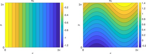
Figure 2. Instability growth rate p for vertical magnetic field as a function of wave number k (with $U_0$, $\ell =0$) for $\nu =\eta =0.4$ (P = 1), and $B_0=0$ (blue), $B_0=0.05$ (red), $B_0=0.10$ (green), $B_0=0.15$ (purple), $B_0=0.20$ (orange) and $B_0=0.25$ (dark orange). Panels (a) and (b) show $\mathrm{Re}\{p\}$ and $\mathrm{Im}\{p\}$, respectively, and dashed curves show the Alfvén wave branch in (28(28) $p=\pm \mathrm{i}k\sqrt{B_0^2-\frac{1}{4}(\nu -\eta {)}^2{k}^2}-\frac{1}{2}(\nu +\eta )k^2,$(28) ) (Colour online).

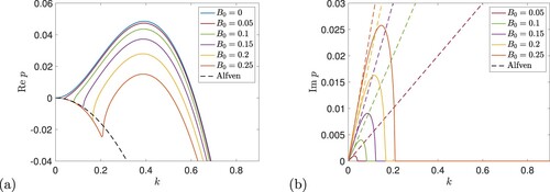
Figure 3. Structure of a typical unstable mode, with $B_0=0.25$, $\nu =\eta =0.4$, k = 0.4; (a) shows the stream function ψ and (b) the magnetic potential a.

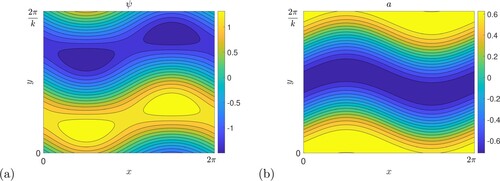
Figure 4. Instability growth rate $\mathrm{Re}\{p_{max}\}$ for vertical field plotted in the $(\nu ,B_0)$ plane for P = 1, $\ell =0$, $U_0=0$, $0.01\le \nu \le 0.8$. Panel (a) shows the numerical computation of growth rates with the threshold $\mathrm{Re}\{p_{max}\}=0$ given by a white curve, and panel (b) the analytical maximum growth rate from (30(30) $p_{max}(\nu ,B_0,P)=-\frac{\sqrt{2}P}{1+P^2}{B}_0^2+\frac{\sqrt{2}}{3}(\frac{1}{\sqrt{2}}-\nu {)}^2,k_{max}^2=\frac{\sqrt{2}}{3}(\frac{1}{\sqrt{2}}-\nu ).$(30) ) and threshold from (31(31) $B_0(\nu ,P)=\sqrt{\frac{1+P^2}{3P}}(\frac{1}{\sqrt{2}}-\nu ).$(31) ). Black shows zero growth rates.

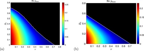
Figure 5. Shown are numerical calculations of (a) the instability growth rate $\mathrm{Re}\{p_{max}\}$ and (b) the frequency $\mathrm{Im}\{p_{max}\}$ for vertical field plotted in the $(\nu ,B_0)$ plane, with $P=1/2$, $0.01\le \nu \le 0.4$. Black shows zero values and the solid white curve in panel (a) shows the numerical threshold $\mathrm{Re}\{p_{max}\}=0$ for instability; the dotted white line in (a) shows the theoretical threshold ${\nu }_{\ast }$ from (35(35) $\nu <{\nu }_{\ast }=\sqrt{\frac{P}{2}\frac{1-P}{1+P}}\mathrm{or}R>R_{\ast }=\sqrt{\frac{2}{P}\frac{1+P}{1-P}}.$(35) ) (Colour online).

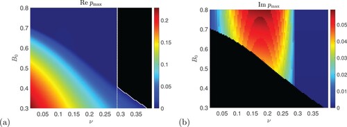
Figure 6. Instability growth rate $\mathrm{Re}\{p\}$ for vertical field as a function of $(\ell ,k)$ for (a) $\nu =\eta =0.4$ (P = 1) with $B_0=0.25$, and (b) $\nu =0.2$, $\eta =0.4$ (P = 0.5) with $B_0=0.7$. The white contour lines give $\mathrm{Re}\{p\}=0$; inside growth rates are positive (Colour online).

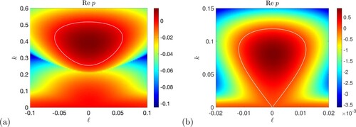
Figure 7. Real positive roots ${\nu }_{\ast }$ of (39(39) $\frac{P}{2}\frac{1-P}{1+P}({\nu }_{\ast }^2-P{U}_0^2)=({\nu }_{\ast }^2+U_0^2)({\nu }_{\ast }^2+P^2{U}_0^2).$(39) ) plotted against P for (a) $0\le P\le 1$ and $U_0=0$ (blue), $U_0=0.04$ (red), $U_0=0.08$ (green), $U_0=0.12$ (purple) and $U_0=0.16$ (orange), and (b) $1\le P\le 5$ and $U_0=0.1$ (blue), $U_0=0.2$ (red), $U_0=0.3$ (green), $U_0=0.4$ (purple) and $U_0=0.5$ (orange). The vertical dashed line is at (a) P = 0.5 and (b) P = 2 (Colour online).

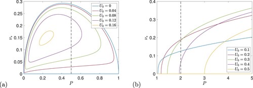
Figure 8. Numerical computations of the instability growth rate $\mathrm{Re}\{p_{max}\}$ for vertical field plotted in the $(\nu ,B_0)$ plane for P = 0.5, $\ell =0$, $0.01\le \nu \le 0.5$ with (a) $U_0=0.12$ and (b) $U_0=0.2$. Black shows zero values and the solid white curve shows the numerical threshold $\mathrm{Re}\{p_{max}\}=0$ for instability; the dotted white lines in panel (a) show the theoretical thresholds ${\nu }_{\ast }$ from (39(39) $\frac{P}{2}\frac{1-P}{1+P}({\nu }_{\ast }^2-P{U}_0^2)=({\nu }_{\ast }^2+U_0^2)({\nu }_{\ast }^2+P^2{U}_0^2).$(39) ) (Colour online).

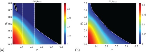
Figure 9. Numerical computations of the instability growth rate $\mathrm{Re}\{p_{max}\}$ for vertical field plotted in the $(\nu ,B_0)$ plane for P = 2, $\ell =0$, with (a) $U_0=0.2$, $0.01\le \nu \le 0.5$ and (b) $U_0=0.4$, $0.01\le \nu \le 0.6$. Black shows zero values and the solid white curve shows the numerical threshold $\mathrm{Re}\{p_{max}\}=0$ for instability; the dotted white line in each panel shows the theoretical threshold ${\nu }_{\ast }$ from (39(39) $\frac{P}{2}\frac{1-P}{1+P}({\nu }_{\ast }^2-P{U}_0^2)=({\nu }_{\ast }^2+U_0^2)({\nu }_{\ast }^2+P^2{U}_0^2).$(39) ) (Colour online).

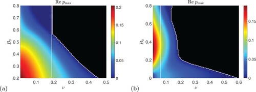
Figure 10. A typical unstable mode, with $U_0=0.2$, $B_0=0.8$, $\nu =0.1$, P = 2, $k=0.08$ from the strong field branch. Panel (a) shows the stream function ψ and (b) the magnetic potential a (Colour online).

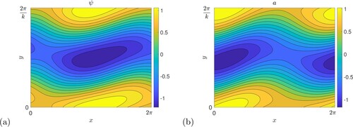
Figure 11. Numerical computations of the instability growth rate $\mathrm{Re}\{p_{max}\}$ for vertical field plotted in the $(\nu ,B_0)$ plane for P = 1, $\ell =0$, with (a) $U_0=0.2$, $0.01\le \nu \le 0.7$ and (b) $U_0=0.5$, $0.01\le \nu \le 0.6$. The numerical threshold $\mathrm{Re}\{p_{max}\}=0$ is given by a white curve and black shows zero growth rates.

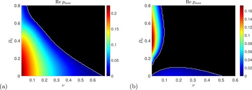
Figure 12. Instability growth rate p for horizontal field as a function of k (and $\ell =0$) for $\nu =\eta =0.1$ (P = 1), with $B_0=0$ (blue), 0.05 (red), 0.1 (green), 0.15 (purple), 0.20 (orange) and 0.25 (dark orange). Panels (a) and (b) show $\mathrm{Re}\{p\}$ and $\mathrm{Im}\{p\}$, respectively (Colour online).

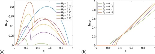
Figure 13. Instability growth rate $\mathrm{Re}\{p_{max}\}$ for horizontal field plotted in the $(\nu ,B_0)$ plane for P = 1, $\ell =0$, $U_0=0$, $0.1\le \nu \le 1$. Panel (a) shows the numerical computation of growth rates with the threshold $\mathrm{Re}\{p_{max}\}=0$ given by the white curve and the stable region in black. In panel (b) we show the analytical thresholds from (48(48) $B_0^2=\frac{{\nu }^2}{P}\frac{1-2{\nu }^2}{P(P+2)+2{\nu }^2}.$(48) ) for the flow branch (blue), and from (52(52) $B_0^2=\frac{{\nu }^2}{P}\frac{P^2+2{\nu }^2}{3P^2-2{\nu }^2}.$(52) ) for the field branch (red). In panel (b) the dashed blue line is the threshold (58(58) $B_0^2=\frac{{\nu }^2}{P}\frac{P(P+2)-{\nu }^2}{P^2+{\nu }^2}.$(58) ) for $\ell \ne 0$ instabilities discussed later. Panels (c, d) show the same as (a, b) but with axes $0.1\le \nu \le 1.25$ and $0\le B\le 5$, and in (c) the asymptote ${\nu }_{\ast }$ from (53(53) ${\nu }_{\ast }=P\sqrt{3/2},$(53) ) is shown dotted.

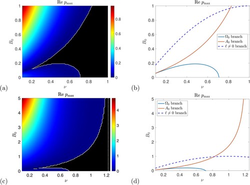
Figure 14. A typical unstable mode, with $B_0=0.05$, $\nu =\eta =0.1$, k = 0.5, from the flow or ${\Omega }_0$ branch; (a) shows the stream function ψ and (b) the magnetic potential a (Colour online).

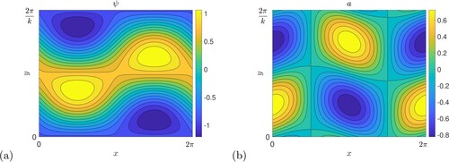
Figure 15. A typical unstable mode, with $B_0=0.25$, $\nu =\eta =0.1$, k = 0.25 from the field or $A_0$ branch; (a) shows the stream function ψ and (b) the magnetic potential a (Colour online).

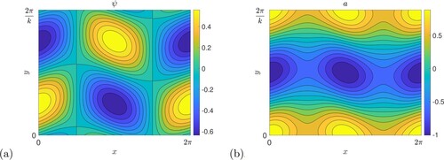
Figure 16. (a) Instability growth rate $\mathrm{Re}\{p_{max}\}$ and (b) imaginary part $\mathrm{Im}\{p_{max}\}$ shown for horizontal field, plotted in the $(\nu ,B_0)$ plane with P = 1, $U_0=0$, any ℓ and $0.1\le \nu \le 1$. The maximising values of $k_{max}$ and of ${\ell }_{max}$ are shown in panels (c, d), respectively. White markers indicate different regions of the diagrams as discussed in the text (Colour online).

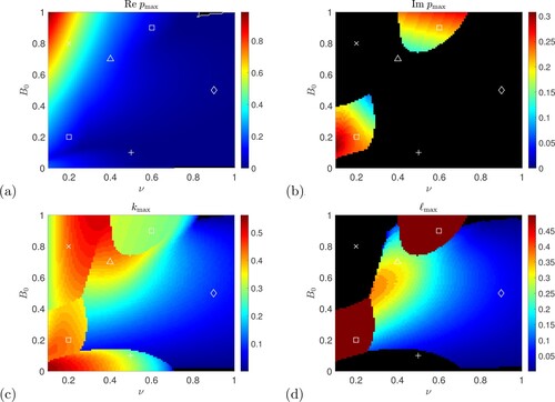
Figure 17. Instability growth rate p for horizontal field as a function of $(\ell ,k)$ for $\nu =\eta =0.75$ (P = 1) with $B_0=0.2$, (a) numerical growth rates and (b) approximate growth rates calculated from (57(57) $\begin{array}{rl}p& =\pm B_0\ell {[\frac{k^2}{{\ell }^2+k^2}\frac{P[{\nu }^2(P+2)-P^2{B}_0^2]}{{\nu }^2({\nu }^2+P{B}_0^2)}-1]}^{1/2}-\frac{1}{2}\nu (1+P^{-1})(k^2+{\ell }^2)\\ & +\mathrm{O}(k^2,{\ell }^2),\end{array}$(57) ). In both panels the white curve is given by $\mathrm{Re}\{p\}=0$, with instability inside this curve, and the straight black lines emerging from the origin are from the formula (56(56) $\frac{k^2}{{\ell }^2}=\frac{{\nu }^2({\nu }^2+P{B}_0^2)}{{\nu }^2(P^2+2P-{\nu }^2)-P{B}_0^2({\nu }^2+P^2)}.$(56) ).

Figure 18. A typical unstable mode, with $\ell =0.05$, k = 0.05, $\nu =\eta =0.75$, $B_0=0.2$; (a) shows the stream function ψ and (b) the magnetic potential a.

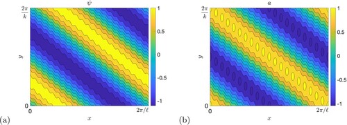
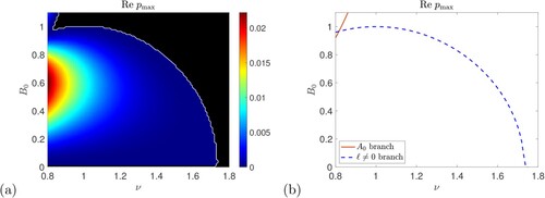
Figure 19. (a) Instability growth rate $\mathrm{Re}\{p_{max}\}$ plotted in the $(\nu ,B_0)$ plane with P = 1, $U_0=0$, and $\ell \ne 0$; (b) shows thresholds (52(52) $B_0^2=\frac{{\nu }^2}{P}\frac{P^2+2{\nu }^2}{3P^2-2{\nu }^2}.$(52) ) for $\ell =0$ (red) and (58(58) $B_0^2=\frac{{\nu }^2}{P}\frac{P(P+2)-{\nu }^2}{P^2+{\nu }^2}.$(58) ) for $\ell \ne 0$ (blue dashed) (Colour online).