Figures & data
Fig. 1 Map of the central west coast of Vancouver Island showing relevant placenames, shelf bathymetry contours (metres), model boundary, offshore weather buoys, and ADCP moorings whose data are used this study.
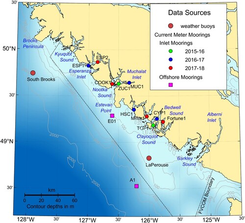
Fig. 2 Horizontal grid for the FVCOM simulations and locations of the tide and pressure gauges used to evaluate the model SSHs. The inset shows a grid close-up of eastern Muchalat Inlet near Gold River.
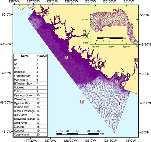
Fig. 3 Comparison of M2 (a) and K1 (b) amplitudes (cm) and phase lags (degrees, UTC) at the twenty comparison sites shown in .
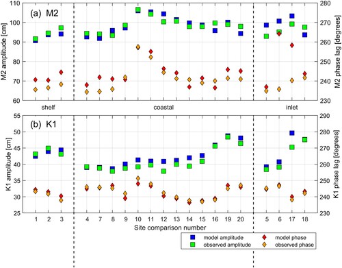
Fig. 4 Hourly, low-pass filtered, observed and model SSHs at Tofino for 4 March to 31 July 2016. Both time series have been normalized so their respective means are zero.
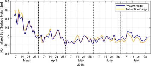
Fig. 5 Observed and model M2 and K1 major semi-axes versus depth at (a) E01, (b) TOF1, and (c) ZUC1 as determined by harmonic analysis of hourly values over 4 March to 11 July 2016. Note scale changes.
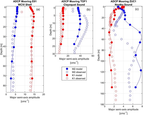
Fig. 6 Model M2 (a) and K1 (b) major semi-axes (cm s−1) at 5 m depth with comparable values from ADCP time series at the bin closest to 5 m, super-imposed as coloured dots. (See for precise ADCP locations.)
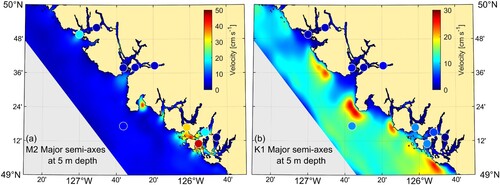
Table 1. M2 and K1 major semi-axes (cm s−1) at the ADCP moorings displayed in and at the bin depths, or FVCOM layer depths, closest to 5 m.
Fig. 7 Along-shelf, low-pass filtered velocity profiles (m s−1) at the E01 mooring for 1 March to 11 July 2016: (a) observed with bottom mounted ADCP, (b) simulated with CIOPS-W model, (c) simulated with FVCOM model. Positive (red) velocities are directed toward 147°counter-clockwise from east and are typically associated with downwelling conditions. Negative (blue) velocities, directed toward 33° clockwise from east, are similarly associated with upwelling conditions. Grey regions denote unreliable observations.
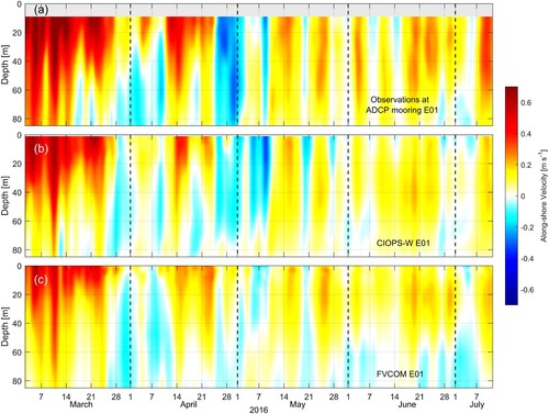
Fig. 11 East-west and north-south components of the wind (m s−1) (left column) and wind roses (right column) at the La Perouse buoy (C46206 in ) for the period of 1 March to 15 July 2016. Row (a) shows the east-west and north-south components from the HRDPS model and the associated wind rose, while row (b) is similar but for the observations. Row (c) displays differences in direction and speed ratios. Dots are hourly values while lines are twelve hour running means. Wind rose directions denote to where the wind is blowing while the polygons denote the average speed in each direction.
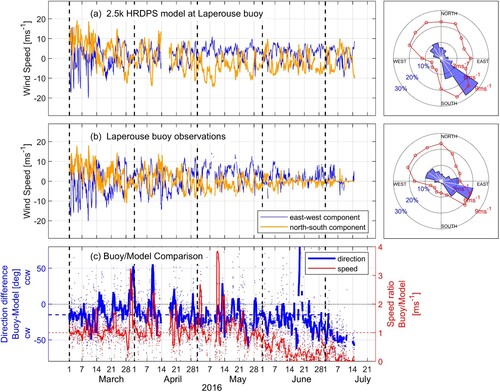
Fig. 8 Along-channel, low-pass filtered velocity profiles (m s−1) at the TOF1 mooring: (a) observed with bottom mounted ADCP, (b) simulated with FVCOM model. Positive velocities are directed toward 57° counter-clockwise from east. Grey regions denotes unreliable observations or missing values due to bathymetric smoothing.
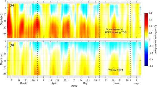
Fig. 9 Along-channel, low-pass filtered velocity profiles (m s−1) at the ZUC1 mooring: (a) observed with bottom mounted ADCP, (b) simulated with FVCOM model. Positive velocities (red) are directed up-inlet toward 71° counter-clockwise from east. Grey regions denote unreliable observations or missing values due to bathymetric smoothing.
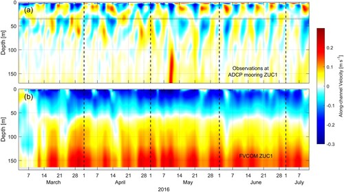
Fig. 10 East-west and north-south components of the wind (m s−1) (left column) and wind roses (right column) at the Saranac Island farm for the period of 23 May to 31 August 2019. Row (a) shows the east-west and north-south components of the observations and the associated wind rose, while rows (b) and (c) are similar but for the HRDPS atmospheric models with 2.5 and 1.0 km horizontal resolution, respectively. Percent wind rose directions denote to where the wind is blowing while the polygons denote the average speed in each direction.
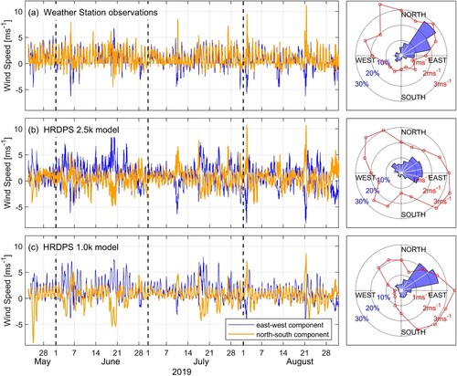
Fig. A1 Locations of the rivers whose volume discharges, temperature, and salinity were used in the model forcing.
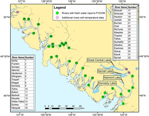
Fig. A2 Observed and estimated river discharges (m s−3) for the period of 1 March to 31 July 2016. WSC observations are shown in the upper panel while estimated values are shown in the lower panel. A log scale has been used to help differentiate small values.
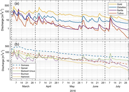
Fig. A3 Daily averaged river temperature (°C), 1 March to 31 July 2016.
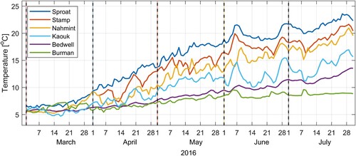
Table A1. Summary of freshwater discharge details used in the March-July 2016 model simulation.
Table B1. Root mean square and average differences (RMS, avdif) between model and farm salinity (S, absolute) and temperature (T, °C) at two depths over the period of 1 March to 31 July 2016. Average differences are model minus observed.
Fig. B1 Locations of salmon farms used in model temperature and salinity evaluations.
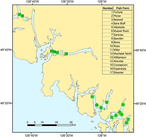
Fig. B2 Observed salinity and temperature at the Williamson Passage farm over the period of 1 March to 31 July 2016.
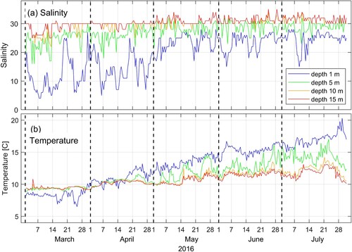
Fig. B3 Observed and modelled salinity (absolute) and temperature (°C) at 1 m depth at the Bare Bluff farm in Bedwell Sound, along with model values interpolated to the same time and depth.
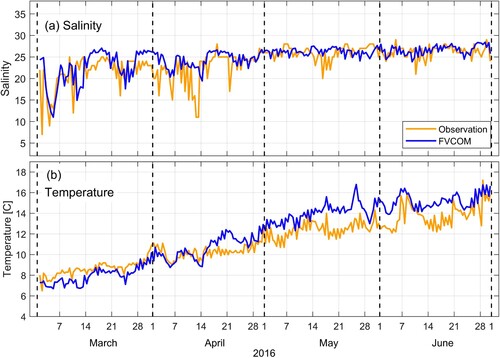
Fig. B4 Model March–May 2016 (a) and observed March–May 2017 (b) salinity at the Muchalat North farm along with corresponding daily discharges for the Gold River.
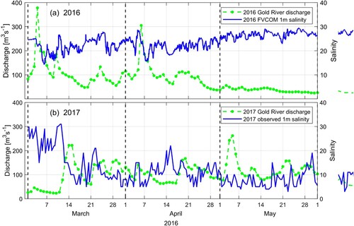
Fig. B5 Near-bottom, half-hourly observed (Microcat) and hourly model (a) absolute salinity and (b) temperature (°C) at E01 for the period of 1 March to 12 July 2016. Analogous daily CIOPS-W values at 97 m depth were interpolated to the boundary node nearest E01 and are also shown.
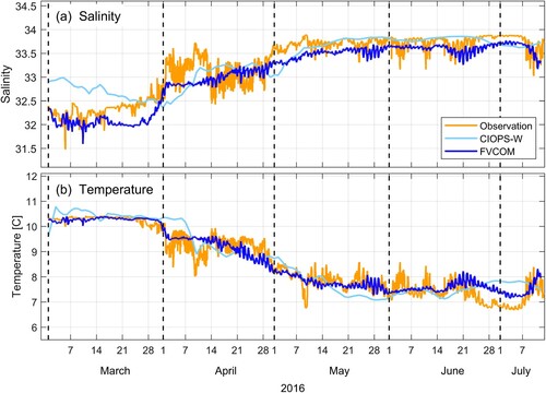
Fig. B6 Bottom observed and model (a) absolute salinity and (b) temperature (°C) at TOF1 for the period of 1 March to 11 July 2016.
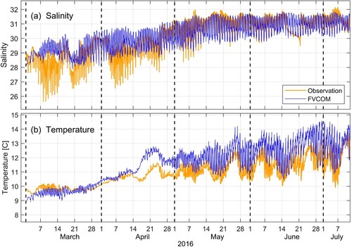
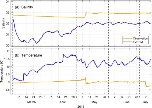
Fig. B7 Model and observed bottom temperature (T, °C) and absolute salinity (S) at the ZUC1 mooring () for the period of 1 March to 12 July 2016.