
Figures & data
Fig. 1 Map of research subareas. The outer edges of these areas are defined by the 200 m isobath. The inset at the top left shows the North Atlantic Ocean, and the location of the research region in this study (blue rectangle), and the solid lines indicate 200, 1000, 3000 m isobaths.
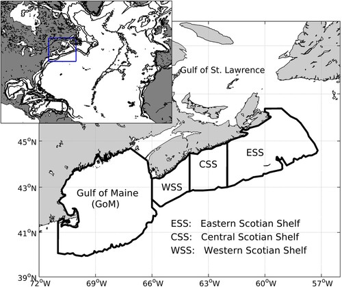
Table 1. Summary of the 22 CMIP6 ESMs.
Table 2. SST: The model bias (Bs; unit: deg) and trends (Tr; unit: deg/decade) for all time series, all calculated from time series of annual means, 1955-2014. Underlined: confidence level < 95%; Blue in brackets (in Tr title cell): trend in HadISST1.
Fig. 2 Time series of annual SST for ensemble mean from the 22 CMIP6 ESMs and HadISST1 data, 1955–2014. The shaded area denotes plus or minus one standard deviation of the 22 models. Units are degrees Celsius.
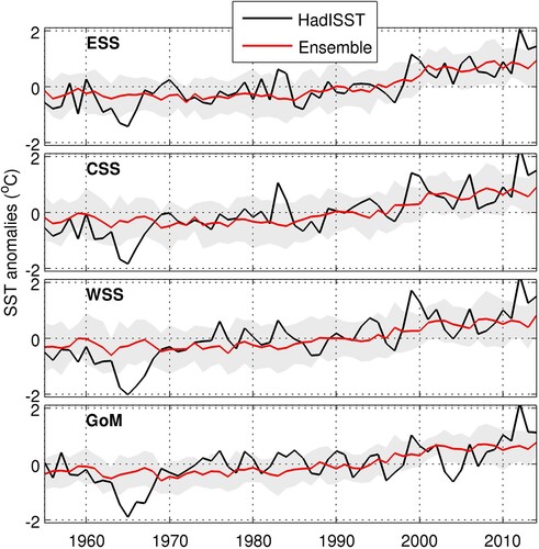
Table 3. July bottom temperature: Model bias (Bs; unit: deg) and trends (Tr; unit: deg/decade) for all time series, 1970-2014. Underlined: confidence level < 90%; Blue in brackets (in Tr title cell): trend values for DFO July survey data.
Fig. 3 Time series of the BT in July from the DFO ecosystem survey data and the ensemble from the 22 CMIP6 ESMs for the period of 1970-2014. The shaded area denotes plus or minus one standard deviation of the 22 models.
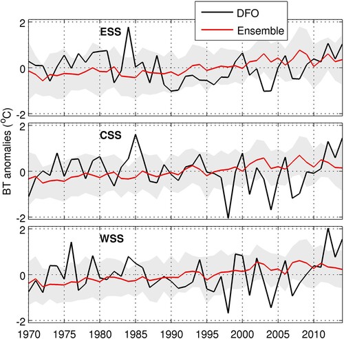
Fig. 4 Violin plots of SST and BT trends for all ESMs (ssp245: light red; ssp370: light blue). The boxes indicate the interquartile range (IQG), and whiskers are 1.5 IQR. The horizontal line is for mean value, and the white circle is for median value.
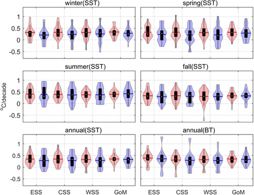
Table 4. Ensemble means of 30-year SST trends from CMIP6 ESMs under ssp245 and ssp370 for the 4 regions. Trends for historic period (1985–2014) are indicated by Hist. Unit: (°C/decade).
Table 5. Projected bi-decadal (bd:2030–2049) and decadal (de: 2040–2049) ensemble mean changes of the SST relative to 1995–2014 period for the ssp245 (s2) and ssp370 (s3). Units are in °C.
Table 6. Ensemble mean trends of annual mean BT for each subarea, for the periods 1985–2014 (Hist) and 2020–2049 (ssp245 and ssp370). Units are °C/decade.
Table 7. Projected bi-decadal (bd:2030–2049) and decadal (de: 2040–2049) annual ensemble mean changes of BT relative to 1995–2014 period for ssp245 (s2) and ssp370 (s3). Units are in °C.