A Circulation Model for Baynes Sound, British Columbia, Canada

Figures & data

Fig. 1 Regional map of Baynes Sound showing CTD stations and locations of ADCP moorings (UB: Union Bay; BCF: BC Ferries) and temperature-salinity time series observations (CM: Comox Marina; LS: Lucky Seven; FB: Fanny Bay; MO: Mac’s Oysters; CI: Chrome Island; HT: Hornby Terminal). The base map showing bathymetric contours (blue) and mudflat regions (green) was modified from the Canadian Hydrographic Service nautical chart #3527. CTD Stations 39 and 40 are outside of map coverage and are located east of Hornby Island roughly extending the line of Stations 35 to 38.

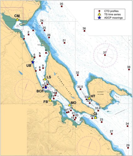
Fig. 2 Triangular grid and bathymetry for the circulation model. (a) for the entire model domain showing the mouths of the Englishman, and Little and Big Qualicum rivers, (b) close-up view of Baynes Sound area with the Courtenay, Trent, Tsable, and Rosewall Rivers included in the model, and (c) bounds of the model vertical layers. Panel (a) includes tide gauge locations later used to evaluate the model: (1) Comox; (2) Little River; (3) Hornby Island; (4) Irvines Landing; and (5) Saltery Bay. Dashed lines in Panel (b) show transect lines across which volume fluxes are later calculated.

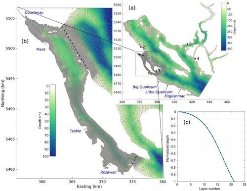
Fig. 3 Chrome Island observed and modelled sea surface salinity (top) and temperature (bottom) for May 2016 to April 2017 superimposed on the average seasonal cycle plus/minus one standard deviation.

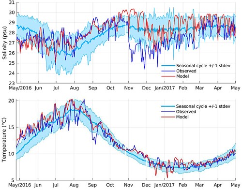
Fig. 4 Average, average plus/minus one standard deviation, and March 1, 2016 to April 30, 2017 Fraser River discharges at Hope.

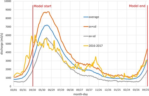
Fig. 5 Average, average plus/minus one standard deviation, and 2016–17 Puntledge River discharges just above its confluence with the Tsolum River just north of Courtenay.

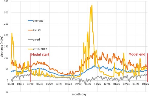
Fig. 6 Salinity and temperature profiles at CTD stations BS2 (left panels) and BS17 (right panels) for April.

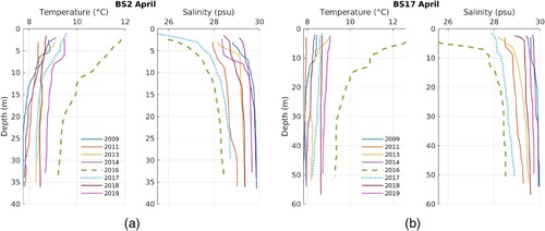
Fig. 7 Salinity and temperature profiles at CTD stations BS2 (left panels) and BS17 (right panels) for June.

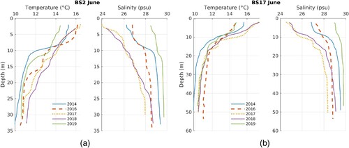
Fig. 8 Temperature profiles observed at CTD stations along the Baynes Sound thalweg during the June 2016 survey (upper panel) corresponding model values (lower panel) at the same locations and time. Station names, dates, and times for each CTD cast are at the top of each panel. Model values were interpolated to coincide with these times. The dashed line is the bottom profile from the model bathymetry, while the grey shaded region denotes the true bathymetry.

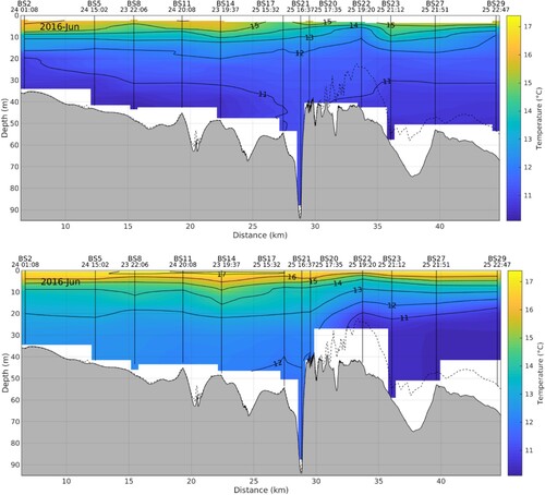
Fig. 9 Salinity profiles observed at CTD stations along the Baynes Sound thalweg during the June 2016 survey (upper panel) and corresponding model values (lower panel) at the same locations and time. Station names, dates, and times for each CTD cast are at the top of each panel. Model values were interpolated to coincide with these times. The dashed line is the bottom profile from the model bathymetry, while the grey shaded region denotes the true bathymetry.

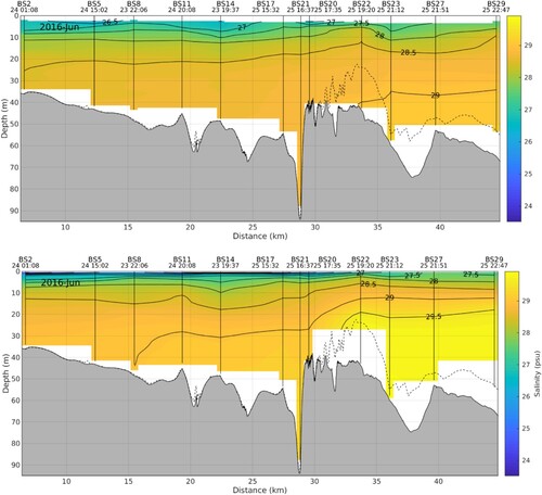
Fig. 10 Observed and model temperature and salinity profiles at CTD station BS17 for April and June 2016 and April 2017 from left to right panels (see Fig. 1). The thick red lines indicate model values at the time of observation while the thin red lines are at 20 min intervals over the day, thus providing an indication of variations over a tidal cycle. Note the different scaling on the x-axes.

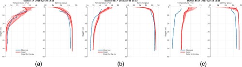
Fig. 11 Observed and modeled temperatures at the five sites (Comox Marina, Fanny Bay Dock, Hornby Terminal, Lucky Seven, Mac’s Oysters) shown with yellow triangles in Fig. 1.

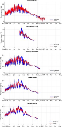
Fig. 12 Rotary spectra versus depth at the BC Ferries ADCP mooring location over the period of February 25 to April 12. Left panels are for the observations in 2012 while the right panels are from the model simulation in 2017. CW and CCW denote clockwise and counter-clockwise components, respectively. Note the frequency axis and power colour legend have logarithmic scaling. Depth is relative to mean sea level.

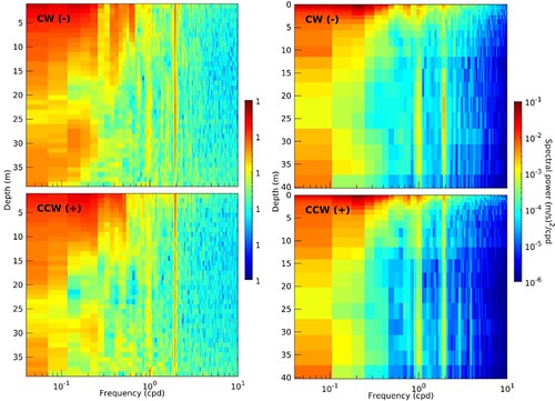
Fig. 13 Rotary spectra versus depth at the Union Bay ADCP mooring location over the period of June 15 to August 30, 2016. Left panels, from observations; right panels, from the model simulation. CW and CCW denote clockwise and counter-clockwise components, respectively. Note the frequency axis and power colour legend have logarithmic scaling. Depth is respect to mean sea level.

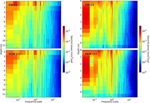
Fig. 14 Ellipses versus depth at the BC Ferries ADCP location: upper panel for M2 and lower panel for K1. The left-most column was computed from the observations over the period of Feb 25 to Apr 12, 2012, while the next four columns were computed from the model currents for the respective periods of JFM2017, MJ2016, JAS2016, and OND2016. Blue ellipses denote vectors that are rotating counterclockwise while red ellipses denote clockwise rotation.

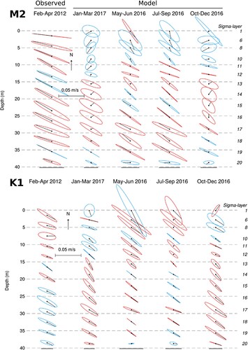
Table 1. Comparison of observed and model amplitudes (m) and phases (degrees) at five tide gauge locations (Fig. 2a) and Union Bay ADCP location (Fig. 1). RMS values were calculated using equation 3 in Cummins and Oey (1997). The asterisked (*) constituents were inferred due to insufficient length of the analyzed time series.

Station	Constituent	Observed		Model
						Discrepancy with observation		RMS
		Amp	Phase	Amp	Phase	Amp	Phase	Abs	Rel (%)
Comox	O1	0.489	264.6	0.484	272.8	0.005	−8.1	0.049	10.0
	K1	0.885	287.5	0.878	286.9	0.007	0.6	0.008	0.9
	N2	0.220	7.7	0.222	11.5	−0.002	−3.8	0.010	4.7
	M2	1.002	33.9	1.009	33.2	−0.008	0.7	0.010	1.0
	S2	0.253	62.6	0.256	53.8	−0.003	8.8	0.028	10.9
Little River	O1	0.496	263.6	0.484	272.6	0.012	−8.9	0.055	11.0
	K1	0.895	288.0	0.877	286.8	0.018	1.2	0.018	2.0
	N2	0.216	3.5	0.220	10.4	−0.004	−7.0	0.019	8.8
	M2	0.984	33.8	1.002	32.2	−0.018	1.6	0.023	2.4
	S2	0.250	63.8	0.254	52.9	−0.004	10.9	0.034	13.6
Hornby Island	O1	0.469	267.6	0.483	272.5	−0.014	−5.0	0.031	6.5
	K1	0.881	288.9	0.875	286.6	0.006	2.3	0.025	2.8
	N2	0.228	10.7	0.219	11.1	0.009	−0.4	0.007	2.9
	M2	0.982	36.5	0.994	32.8	−0.013	3.7	0.046	4.7
	S2	0.262	65.6	0.253	53.5	0.010	12.2	0.039	15.0
Irvines Landing	O1	0.483	263.8	0.484	271.9	0.000	−8.1	0.048	10.0
	K1	0.892	286.4	0.878	285.9	0.014	0.5	0.011	1.3
	N2	0.213	5.5	0.218	10.7	−0.005	−5.2	0.014	6.7
	M2	0.987	32.3	0.992	32.5	−0.005	−0.2	0.004	0.4
	S2	0.248	61.4	0.252	53.2	−0.004	8.2	0.026	10.3
Saltery Bay	O1	0.481	264.7	0.487	272.3	−0.006	−7.5	0.045	9.4
	K1	0.873	287.7	0.883	286.4	−0.011	1.3	0.016	1.8
	N2	0.226	5.7	0.223	11.4	0.003	−5.6	0.016	7.0
	M2	0.996	32.9	1.014	33.1	−0.018	−0.2	0.013	1.3
	S2	0.244	63.1	0.258	53.9	−0.014	9.2	0.030	12.4
Union Bay	O1	0.490	267.3	0.493	271.8	−0.003	−4.5	0.027	5.5
	K1*	0.838	289.6	0.759	275.9	0.079	13.7	0.145	17.3
	N2	0.176	2.9	0.223	12.0	−0.046	−9.1	0.040	22.4
	M2	0.970	33.1	1.010	33.5	−0.040	−0.5	0.029	3.0
	S2*	0.233	60.3	0.276	46.1	−0.043	14.2	0.054	23.0

Fig. 15 K1 (top) and M2 (bottom) semi-major axes at 1-metre depth as calculated from harmonic analysis of model currents for the period of May 1 to October 31, 2016.

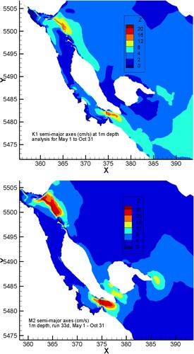
Fig. 16 Observed water temperature, model daily range in sea surface elevation, and air temperature and wind components along and cross the axis of Baynes Sound from HRDPS at Mac’s Oysters site for the period of May to November 2016.

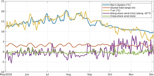
Fig. 17 Lag time relationships between observed water temperature and i) tidal range (left graph), ii) air temperature (middle graph), and iii) wind (right graph).

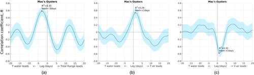
Table 2. Partial least squares regression of the observed and the model water temperature on the diurnal tidal range, air temperature, and wind speed at CTD probe stations: Predictor lead/lag period (days) and associated coefficient of determination (r²).

Station/Predictor	Predictor lead (+)/lag (−)		Total r^2		Partial r^2		Individual r^2
	Obs	Model	Obs	Model	Obs	Model	Obs	Model
Comox Marina			0.59	0.45
Tidal Range	6	−3			0.11	0.01	0.28	0.15
T air	1	1			0.13	0.05	0.28	0.15
V air	1	2			0.13	0.24	0.30	0.36
Hornby Terminal			0.56	0.27
Tidal Range	5	6			0.13	0.01	0.26	0.06
T air	1	1			0.08	0.10	0.19	0.18
V air	1	1			0.16	0.07	0.35	0.14
Lucky Seven			0.61	0.50
Tidal Range	−3	−2			0.11	0.04	0.34	0.23
T air	2	2			0.11	0.11	0.27	0.27
V air	2	2			0.13	0.14	0.32	0.29
Mac’s Oysters			0.60	0.49
Tidal Range	−3	−3			0.09	0.04	0.34	0.21
T air	1	2			0.08	0.13	0.28	0.27
V air	1	2			0.15	0.12	0.33	0.27

Fig. 18 Observed water temperature at the Mac’s Oysters location along with hindcasts based on regressions with each and all of the spring-neap tidal cycle, air temperature, and along-shore wind as predictors.

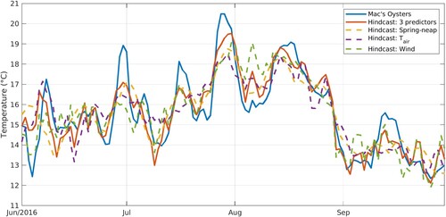
Fig. 19 Average velocity (m s⁻¹) profiles along a transect (Fig. 2b) crossing the northern entrance to the Sound for the four seasons: spring (April-May-June), summer (July-August-September), fall (October-November-December), and winter (January-February-March). Red = incoming, blue = outgoing, y-axis is depth (m), x-axis is transect distance (m), measured from Denman Island.

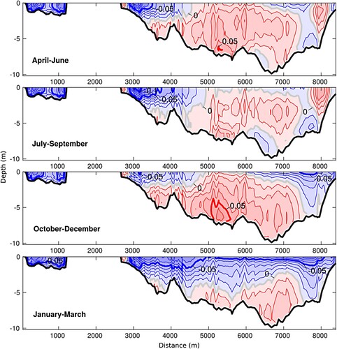
Fig. 20 Average seasonal velocity (m s⁻¹) profiles across a transect at the southern entrance to Baynes Sound (see Fig. 2b for transect location). X-axis is distance measured from Vancouver Island. Red = incoming, blue = outgoing.

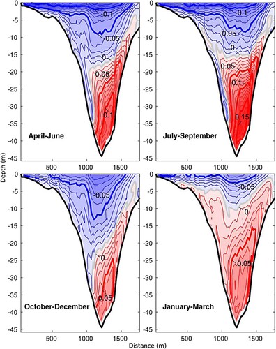
Table 3. Average seasonal volume transports (m³s⁻¹) crossing the northern and southern entrances to Baynes Sound, and estimated balances corresponding to the velocities shown in Figs. 20 and 21. AMJ = April, May, June; JAS = July, August, September; OND = October, November, December; JFM = January, February, March.

Season	North			South			Rivers	Balance
	inflow	outflow	net	inflow	outflow	net
AMJ	545	−321	224	566	−870	−304	67	−13
JAS	277	−393	−116	827	−757	70	33	−14
OND	646	−270	376	305	−778	−473	84	−13
JFM	177	−693	−516	690	−267	423	80	−12
Year	412	−418	−6	596	−670	−73	66	−13

Fig. 21 Spatial distribution of water renewal time (WRT) in the surface (left) and bottom (right) layers of Baynes Sound.

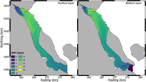
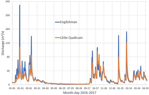
Fig. 22 Englishman and Little Qualicum River discharges (m³ s⁻¹) for the period of January 1, 2016 to April 30, 2017.

Cummins, P. F., & Oey, L. Y. (1997). Simulation of barotropic and baroclinic tides off northern British Columbia. Journal of Physical Oceanography, 27(5), 762–781. https://doi.org/10.1175/1520-0485(1997)027%3C0762:SOBABT%3E2.0.CO;2

 Web of Science ®Google Scholar