A Deep Learning Model with Axial Attention for Radar Echo Extrapolation

Figures & data

Figure 1. The illustration of Axial attention. The left part represents horizontal attention. X represents the input feature map, and $W_{\mathit{hq}}$,$\mathit{\hspace{0.17em}}{W}_{\mathit{hk}}$ and $W_{\mathit{hv}}\mathit{\hspace{0.17em}}$refer to weight matrices of query, key and value for horizontal attention, and $W_{\mathit{vq}}$,$\mathit{\hspace{0.17em}}{W}_{\mathit{vk}}$ and $W_{\mathit{vv}}\mathit{\hspace{0.17em}}$refer to weight matrices of query, key and value for vertical attention. $E^{\mathit{w}\times \mathit{H}\times \mathit{H}}$ and $E^{\mathit{H}\times \mathit{w}\times \mathit{w}}$ represent the similarity matrix. $P_h$ and $P_v$ is attention by multiplying E with V. $W_{\mathit{ho}}$ and $W_{\mathit{vo}}$ is a convolutional kernel, and $\mathit{A}{T}_h$ denotes the output of horizontal attention. The right part represents vertical attention $\mathit{A}{T}_v$ and at represents the output of the attention module.

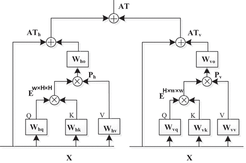
Figure 2. The illustration of the TrajGRU unit. $X_t$ represents the input, $H_{\mathit{t}-1}$ represents the hidden state at time step t-1. γ denotes the sub-network within the TrajGRU model, which includes two convolutional recurrent neural networks (conv). Warp is the function used to select the dynamic connections. ${\tilde{H}}_{\mathit{t}-1}$ is the updated hidden state at time step t-1. GRU represents a GRU neural network model, and $H_t$ represents the hidden state at time step t.

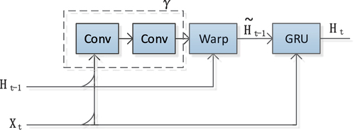
Figure 3. The illustration of the SA-TrajGRU unit. $X_t$ represents the input, and $H_{\mathit{t}-1}\mathit{\hspace{0.17em}}$represents the hidden state at time step t-1. At denotes the attention layer, and $\tilde{\gamma }$ represents the sub-network of the SA-TrajGRU unit, which includes two convolutional recurrent neural networks (conv) and the attention layer (AT). Warp is the function used to select the dynamic connections.$\mathit{\hspace{0.17em}}{\tilde{H}}_{\mathit{t}-1}$ represents the updated hidden state at time step t-1. GRU represents a GRU neural network model, and $H_t$ represents the hidden state at time step t.

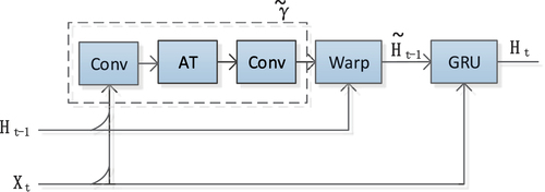
Figure 4. Encode-decode architecture based on SA-TrajGRU units. $X_{\mathit{t}-1}$ and $X_t$ represent the input, while ${\tilde{X}}_{\mathit{t}+1}$ and ${\tilde{X}}_{\mathit{t}+2}$ represent the output. Conv refers to the convolution block, and SA-TrajGRU represents the SA-TrajGRU unit, and Deconv represents the deconvolution block.

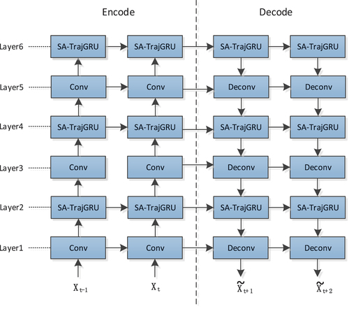
Table 1. The details of the SA-TrajGRU model.

Part	Layer	Kernel	Stride	Ch I/O	Type
Encode	Layer1	3×3	2	1/16	Conv
	Layer2	3×3	1	16/32	SA-TrajGRU
	Layer3	3×3	2	32/64	Conv
	Layer4	3×3	1	64/32	SA-TrajGRU
	Layer5	3×3	2	32/16	Conv
	Layer6	3×3	1	16/16	SA-TrajGRU
Decode	Layer6	3×3	1	16/16	SA-TrajGRU
	Layer5	3×3	2	16/32	Deconv
	Layer4	3×3	1	32/64	SA-TrajGRU
	Layer3	3×3	2	64/32	Deconv
	Layer2	3×3	1	32/16	SA-TrajGRU
	Layer1	3×3	2	16/1	Deconv

Figure 5. Frame-wise MSE comparisons of different models on the moving MNIST-2 test set. The numbers following the model names in the captions represent the average values of MSE.

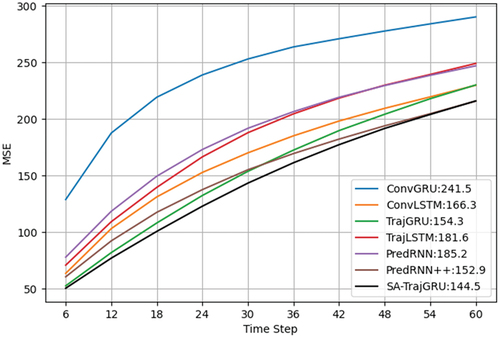
Figure 6. Prediction case on the moving MNIST-2 test set.

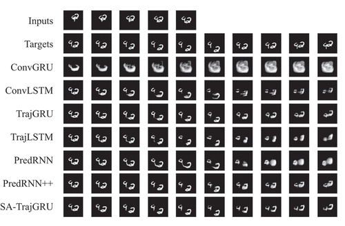
Table 2. Comparison of the average rainfall-RMSE scores of different models.

Precipitation intensity	Rainfall-RMSE(mm/h)
ConvGRU	35.574
ConvLSTM	5.346
TrajGRU	5.290
TrajLSTM	5.273
PredRNN	5.244
PredRNN++	5.170
PFST-LSTM	5.328
SA-TrajGRU	5.115

Table 3. Correspondence between dBZ and precipitation intensity.

Precipitation intensity	dBZ	Precipitation intensity (mm/h)
Light Rain	15–30	.2–2.0
Moderate Rain	30–40	2.0–10
Heavy Rain	40–45	10–30
Torrential Rain	46–50	30–50
Severe Rain	50–55	50–100
Extreme Rain	56–70	>100

Figure 7. HSS and CSI scores of different nowcast lead time. (a) HSS τ = 25 dBZ. (b) CSI τ = 25 dBZ. (c) HSS τ = 35 dBZ. (d) CSI τ = 35 dBZ. (e) HSS τ = 45 dBZ. (f) CSI τ = 45 dBZ.

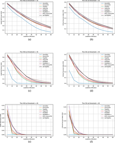
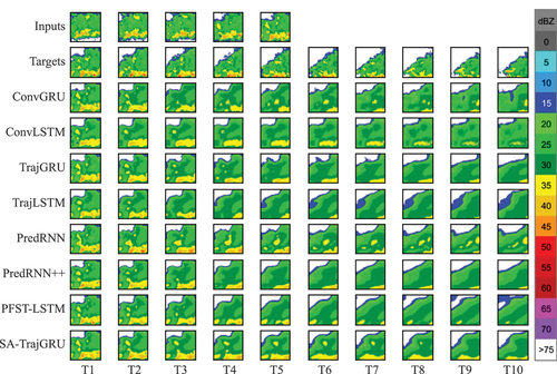
Figure 8. Prediction case of convective precipitation on the CIKM AnalytiCup 2017 test set.

Data availability statement

The data that support the findings of this study are available the Tianchi Laboratory website on Alibaba Cloud. Data are available at https://tianchi.aliyun.com/dataset/1085 with the permission of Alibaba.