Robust Risk-Aware Option Hedging

Figures & data

Figure 1. Depictions of $\gamma \left(u\right)$ for $\alpha =0.2$ and $\text{β}=0.9$ as p varies.

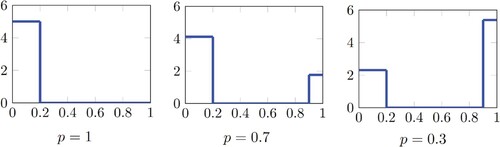
Figure 2. A comparison between trained non-robust strategies (blue) and Black–Scholes delta hedging (orange) for the knock-in call option. The top panel shows post-knock in strategies, while the bottom panels shows pre-knock in strategies.

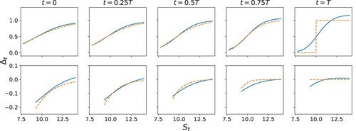
Figure 3. A comparison between robust (red) and non-robust (blue) strategies for the knock-in call option. The top panel shows post-knock in strategies, while the bottom panels shows pre-knock in strategies.

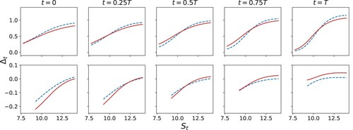
Figure 4. A comparison between robust (red) and non-robust (blue) strategies for the knock-out option. The top panel shows post-knock out strategies, while the bottom panels shows pre-knock out strategies.

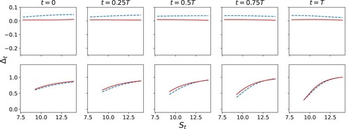
Figure 5. Strategies for hedging the down-and-in call option with transaction costs (TC) and with no transaction costs (NTC) built into the model. (a) Optimal ${\mathrm{\Delta }}_t$ for two sample asset paths and (b) Histogram of total variation of $({\mathrm{\Delta }}_t{)}_{t=0,1\dots N-1}$ across multiple asset paths.

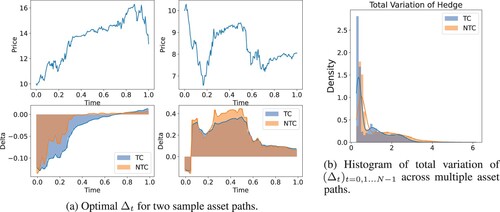
Figure 6. Comparison of Black–Scholes option hedging (Bl–Sch) and robust (Rob) P&L with transaction cost when model is misspecified with $\kappa =1$ and $\rho =-0.1$ in reality. CVaR${}_{0.2}$ is also shown. (a) Knock-in Option and (b) Knock-out option.

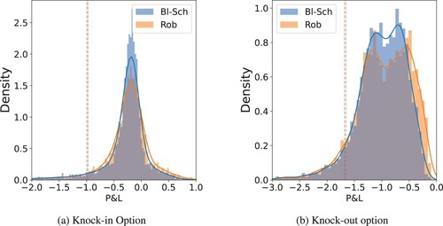
Table 1. Comparison of different pricing schemes.

	Knock-in Call		Knock-Out Call
	Price	${\mathrm{CVaR}}_{0.2}$	Price	${\mathrm{CVaR}}_{0.2}$
$P^{\mathrm{Rob}}$	0.32258	$-0.68025$	1.16839	$-0.51235$
$P^{\mathrm{BS}}$	0.31434	$-0.74954$	1.11398	$-0.60988$
$C^{\mathrm{BS}}$	0.27300	–	0.98123	–

Note: The left column under each header shows the price outputted by the misspecified model targeting CVaR${}_{0.2}=-0.5$. The right column shows the CVaR of a strategy charging their respective price under the actual model.

Figure 7. Non robust hedging strategies for a down-and-in call option. The graph show total asset holdings at t = 0.5T.

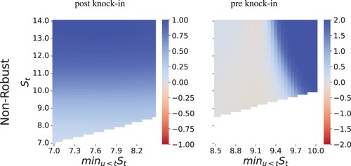
Figure 8. Robust hedging strategies for a down-and-in call option. The graph show total asset holdings at t = 0.5T.

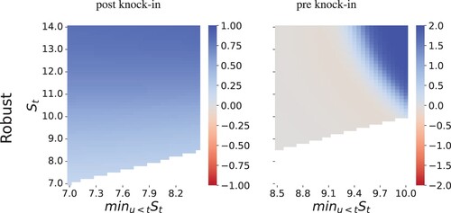
Figure 9. Non robust hedging strategies for a down-and-out call option. The graph show total asset holdings at t = 0.5T.

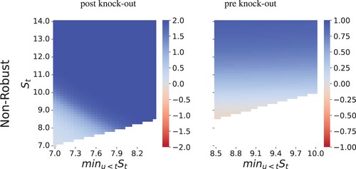
Figure 10. Robust hedging strategies for a down-and-out call option. The graph show total asset holdings at t = 0.5T.

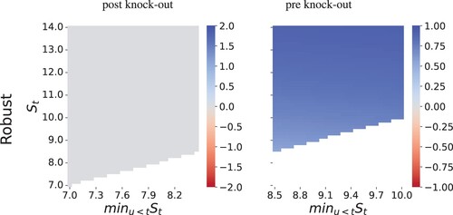
Figure 11. Comparison of total Variation of the hedge position across different asset price paths in cases with transaction costs (TC) and without transaction costs (NTC). (a) Knock-in option and (b) Knock-out option.

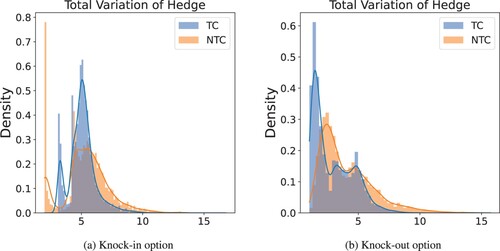
Figure 12. Comparison of non-robust(N-Rob) and robust (Rob) strategies. $-{\mathcal{R}}_g^U\left[X^{\theta }\right]$ is shown as dotted lines in both plots. To help with visualizations, the x-axis uses a symmetric logarithmic scale, with values inside $[-1,1]$ displayed on a linear scale. (a) Knock-in Option and (b) Knock-out option.

Figure 13. ${\mathrm{\Delta }}_i$ along two sample paths for knock-in (above) and knock-out (below) options. Strategies shown correspond to p = 1, 0.85 and 0.70.

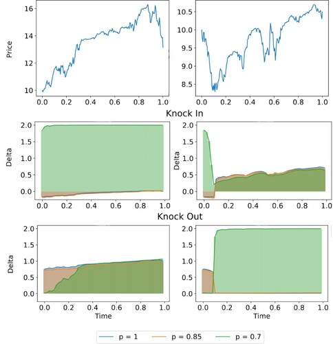
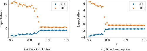
Figure 14. Comparison of lower tail expectation (LTE) and upper tail expectation (UTE) for $\alpha =0.1$ and $\text{β}=0.9$ while varying p. (a) Knock-in Option and (b) Knock-out option.