Monte Carlo Simulation for Trading Under a Lévy-Driven Mean-Reverting Framework

Figures & data

Figure 1. For the spread process X (black line), a trade is entered when the price passes $\pm d$, whichever happens first (red lines), and exited when it passes $\pm c=0$ (blue line). The value of the spread at the entry (red point) and exit (blue point) times are shown. Here, $X\sim \mathrm{OU}\text{-}\mathrm{VG}(1,5,0,0.015,0)$.

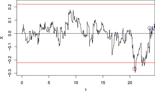
Figure 2. Estimated variance reduction factor R as a function of the number of time points for the control variates p. The parameters are $(\lambda ,b,\mu ,{\sigma }^2,\eta )=(1,1,-0.5,0.015,0.5)$, $X_0=0$, $\gamma =0.1$, r = 0.01.

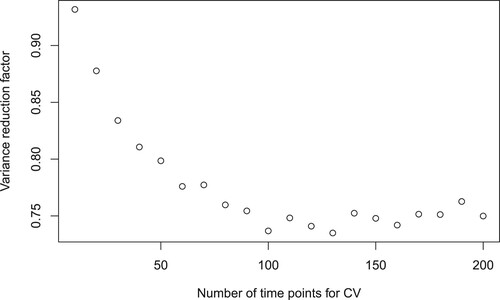
Figure 3. The estimate ${\hat{V}}_C(d)$ of the value function $V(d)$ and the optimal entry level $d^{\ast }=1.086$. The parameters are $(\lambda ,b,\mu ,{\sigma }^2,\eta )=(1,1,-0.5,0.015,0.5)$, $X_0=0$, $\gamma =0.1$, r = 0.01.

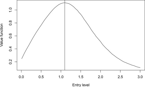
Table 1. For various values of $(b,\mu )$, the optimal number of time points for the control variates $p^{\ast }$ (searching over $p=10,20\dots ,200$) and the optimal variance reduction factor $R^{\ast }$ are shown.

b	μ	$p^{\ast }$	$R^{\ast }$
3	$-$0.05	70	0.951
2	$-$0.05	120	0.904
1	$-$0.05	100	0.871
1	$-$0.5	130	0.735
1	$-$1	110	0.826

Notes: The other parameters are $(\lambda ,{\sigma }^2)=(1,0.015)$, $X_0=0$, $\gamma =0.1$, r = 0.01.

Figure 4. The estimate of the value function $V(d)$ (solid lines) and the corresponding loess smooth (dashed lines) with (red lines) and without (black lines) control variates. The optimal entry level is $d^{\ast }=0.506$ without using control variates, and $d^{\ast }=0.456$ using the optimal number of control variates $p^{\ast }=1$. The parameters are $(\lambda ,b,\mu ,{\sigma }^2,\eta )=(0.01,50,0.5,4,-0.5)$, $X_0=0$, $\gamma =0.1$, r = 0.01.

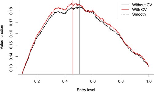
Figure 5. A sample path of the spread $X\sim \mathrm{OU}\text{-}\mathrm{VG}(1,5,-0.5,0.015,0.5)$ using the optimal entry levels in the first row of Table 2.

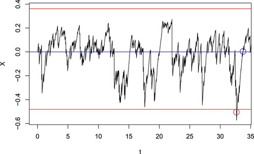
Table 2. For various value of μ, the optimal entry levels $d_{+}^{\ast }$ and $d_{-}^{\ast }$ are shown.

μ	$\mathrm{Skew}(Y)$	$d_{+}^{\ast }$	$d_{-}^{\ast }$
−0.5	−0.825	0.362	0.488
−0.2	−0.660	0.231	0.293
−0.05	−0.225	0.213	0.227
0	0	0.220	0.220

Notes: The other parameters are $(\lambda ,b,{\sigma }^2)=(1,5,0.015)$, $X_0=0$, $\gamma =0$, r = 0.01.

Figure 6. The estimate of the value function $V(c,d)$ with entry level d and exit level c. The parameters are $(\lambda ,b,\mu ,{\sigma }^2,\eta )=(1,5,0,0.015,0)$, $X_0=0.25$, $\gamma =0$, r = 1.

Figure 7. The optimal exit level $c^{\ast }$ for various value of discount rate $r=0.01,0.1,0.2,\dots ,1.5$. The other parameters are $(\lambda ,b,\mu ,{\sigma }^2,\eta )=(1,5,0,0.015,0)$, $X_0=0.25$, $\gamma =0$.

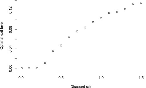
Figure 8. A sample path of the spread $X\sim \mathrm{OU}\text{-}\mathrm{VG}(1,b,0,0.015,0)$, where (a) b = 1 and (b) b = 100, using the optimal entry levels in the first and third row of Table 3.

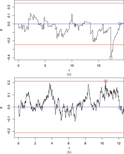
Table 3. For various values of b, the optimal entry level d, the estimate ${\hat{V}}_M(d^{\ast })$ of the optimal expected profit, and overshoot statistics are shown.

b	$d^{\ast }$	${\hat{V}}_M(d^{\ast })$	Sample mean O	Sample sd O
1	0.246	0.286	0.0640	0.0682
5	0.220	0.227	0.0282	0.0306
100	0.211	0.196	0.0086	0.0086

Notes: The other parameters are $(\lambda ,\mu ,{\sigma }^2,\eta )=(1,0,0.015,0)$, $X_0=0$, $\gamma =0$, r = 0.01.

Table 4. For various values of ρ, the optimal entry levels $d_1^{\ast },d_2^{\ast }$, the estimate ${\hat{V}}_M(d_1^{\ast },d_2^{\ast })$ of the optimal expected profit, and the estimated probability of which spread $X_1,X_2$ is traded are shown.

ρ	0.9	0.3	0	−0.3	−0.9
$\mathrm{Corr}(X_1(t),X_2(t))$	0.356	0.119	0	−0.119	−0.356
${\hat{V}}_M(d_1^{\ast },d_2^{\ast })$	0.334	0.335	0.336	0.336	0.334
$d_1^{\ast }$	0.318	0.311	0.305	0.316	0.316
$d_2^{\ast }$	0.338	0.345	0.343	0.334	0.345
Trades only $X_1$ (%)	11.42	14.15	15.88	12.72	12.40
Trades only $X_2$ (%)	83.08	80.34	79.46	83.15	81.38
Trades both (%)	0.97	0.76	0.58	0.56	0.74
Trades neither (%)	4.53	4.75	4.08	3.57	5.48

Notes: The other parameters are given in (16(16) $\begin{array}{rl}\lambda & =1,a=2.5,\mathit{\alpha }=\left(\begin{array}{c}0.2\\ 0.3\end{array}\right),\mathit{\mu }=\left(\begin{array}{c}0\\ -0.2\end{array}\right),\mathrm{\Sigma }=\left(\begin{array}{cc}0.015& \rho \sqrt{{\mathrm{\Sigma }}_{11}{\mathrm{\Sigma }}_{22}}\\ \ast & 0.02\end{array}\right),\end{array}$(16) ) with ${\mathbf{X}}_0=\mathbf{0}$, $\gamma =0$, r = 0.01.

Table 5. For various value of ρ, the optimal entry level $d^{\ast }$ and the estimate ${\hat{V}}_M(d^{\ast })$ of the optimal expected profit.

ρ	0.99	0.9	0.3	0	$-0.3$	$-0.9$
$\mathrm{Corr}(X_1(t),X_2(t))$	0.988	0.898	0.299	0	$-0.299$	$-0.898$
${\hat{V}}_M(d^{\ast })$	0.032	0.035	0.039	0.040	0.040	0.034
$d^{\ast }$	0.037	0.044	0.045	0.045	0.044	0.045

Notes: The other parameters are given in (17(17) $\lambda =1,a=6.65,\mathit{\alpha }=\left(\begin{array}{c}0.15\\ 0.15\end{array}\right),\mathit{\mu }=\mathbf{0},\mathrm{\Sigma }=\left(\begin{array}{cc}0.015& \rho \sqrt{{\mathrm{\Sigma }}_{11}{\mathrm{\Sigma }}_{22}}\\ \ast & 0.015\end{array}\right),$(17) ) with ${\mathbf{X}}_0=\mathbf{0}$, $\gamma =0$, r = 1.