Productivity and cost analysis of cable yarding operations in flat terrain in the canton of Aargau in Switzerland

Figures & data

Figure 1. Position, length and inclination of the cable corridors at the three study sites (top); locations of the study sites in the Swiss canton of Aargau (bottom, left); and location of the study sites within Switzerland (bottom, right). Reproduced with permission from Swisstopo (JA100118).

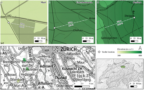
Table 1. Overview of the three study sites in the Swiss canton of Aargau.

Indicator	1-Muri	2-Unterlunkhofen	3-Berikon
Extraction direction	Horizontal	Horizontal	Horizontal
Full name	Muri	Unterlunkhofen	Berikon
Abbreviation	M	U	B
Dates of time study	07–10 March 2022	14–16 February 2023	16–23 February 2023
Size of area (ha)	0.75	1.05	1.1
Dominant species	Broadleaved	Broadleaved	Conifer
Stand composition	Ash, sycamore maple, wild cherry, spruce	Beech, sycamore maple, pedunculate oak	Beech, spruce, sycamore maple
Total volume extracted*	270	150	380
Silvicultural treatment	Final felling clearcut method	Moderate intensity selective cut	High intensity selective cut

**Cubic meters over bark m³ob.

Table 2. Overview of the peculiarities of each study site.

Study site	Description
1 – Muri	There is intermittent waterlogging, with flooding or groundwater upwelling from nearby ponds and fen areas during several days per year. Driving on the logging roads would lead to rut formation, even under ideal conditions. In addition, the stand is affected by ash dieback, and there has been storm and subsequent bark beetle damage in recent years. Due to the ash shoot dieback, there was a need for action regarding logging, especially given the busy cantonal road running directly along the stand. Therefore, the decision was made to clearcut this area. Some seed trees were left standing. As there was no anchor tree, three deadman anchors and one tractor were needed as anchor points.
2 – Unterlunkhofen	The site was affected by a summer storm in July 2021, which blew down mainly beech and sycamore trees with a diameter at breast height (DBH) > 50 cm. In addition, the crowns of spruce and fir trees with a DBH of 40–60 cm were snapped off. The implemented intervention was done as salvage logging after the storm, as well as a light thinning in some parts. Due to the risk of waterlogging, large-scale interventions should be avoided on the site. The former strip roads are clearly visible.
3 – Berikon	No further peculiarity except that the terrain is wet and sensitive to traffic. Strong thinning with a small-scale clearcut around the cable corridor was carried out. Some seed trees were left standing.

Figure 2. Installation of the mobile cable-based system with a Koller tower yarder at the Muri (M) study site.

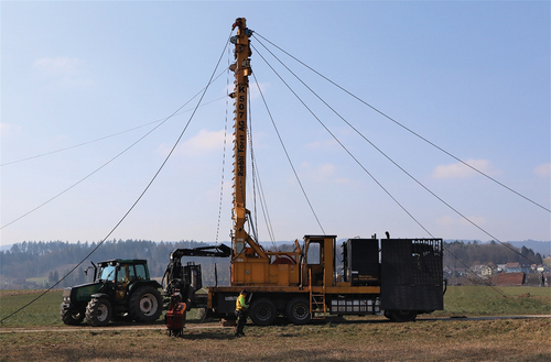
Table 3. Specifications of the cable-based extraction machines K507 and Mounty 40–3.

Features	K 507	Mounty 40–3
Manufacturer	Koller	Konrad
Skyline drum capacity (m)	800	800
Skyline diameter (mm)	22	20
Mainline drum capacity (m)	1350	800
Mainline diameter (mm)	12	12
Haulback line* drum capacity (m)	1350	1600
Haulback line* diameter (mm)	12	11
Tower height (m)	11	13
Carriage model	MSK-3	Liftliner
Maximum pulling capacity (kN)	30	40
Processor	-	Woody 60

*In all cases, a three-cable configuration was used. In contrast to a two-cable configuration, which consists of cable yarders with a skyline and a mainline and can be used for downhill logging only, this configuration additionally includes a haulback line and thus is capable of uphill and flat-terrain logging (see also Figure 1(b) in Varch et al. (2021)).

Table 4. Overview of the forest operations conducted in the three study sites.

	Study Site
Parameter	1-Muri	2-Unterlunkhofen	3-Berikon
Corridor length (m)	189	298	220
Yarding
Type of yarder	Koller K 507	Konrad Mounty 40–3	Konrad Mounty 40–3
Type of carriage	Koller MSK-4	Konrad Liftliner LL40–2	Konrad Liftliner LL40–2
Processing	Motor manually	Processor	Processor
Piling	Forestry tractor HSM 704	-

Figure 3. Mobile cable-based system with a Konrad tower yarder at the Unterlunkhofen (U) study site.

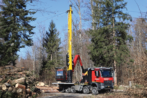
Figure 4. Mobile cable-based system with a Konrad tower yarder at the Berikon (B) study site.

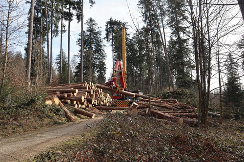
Table 5. Analyzed predictors of productivity response variables.

Predictor	Label	Unit	Description
Yarding distance	yard_dist	m	Distance between yarder processor and carriage
Lateral yarding distance	latyard_dist	m	Distance from tree/tree length to middle of corridor measured at a right angle
Lateral yarding difficulty	latyard_diff	1–low 2–medium 3–high	Lateral yarding difficulty due to terrain (considering microtopography, regeneration/ground cover, stand density, block overlays and slope gradient)
Pieces per cycle	load_pieces_no	no.	Number of trees/tree sections per cycle
Payload	payload	m^3 ob	Volume per cycle
Average piece volume	avrg_piece_volume	m^3 ob	Average volume per tree/tree section
Person yarding	resp_person_yard_proc	person	Operator of the tower yarder processor
Person lateral yarding	resp_person_latyard	person	Forest worker operating in the field and responsible for attaching loads

Table 6. Productivity response variables expressed as cubic meters over bark extracted per productive machine hour (m³ ob PMH₁₅^−1.).

Response variable	Label	Formula
Productive yarding productivity	yard_prod_prod	payload * yard_prod_t^−1 * h
Total yarding productivity (including delays)	yard_tot_prod	payload * yard_tot_t^−1 * h
Lateral yarding productivity	latyard_prod	payload * latyard_t^−1 * h
Productive processing productivity	proc_prod_prod	payload * proc_prod_15_t^−1 * h

yard_prod_t⁻¹ = productive yarding time; yard_tot_t⁻¹ = total yarding time; latyard_t⁻¹ = lateral yarding time; proc_prod_15_t⁻¹ = total processing time including delays of up to 15 minutes; h = hour.

Table 7. Model overview with response variable, predictors and key properties. The models are written in the following way in R (example for #1UB): log(yard_tot_prod) ~ latyard_dist + latyard_diff + log(yard_dist) + log(avrg_piece_volume) + log(payload). The following significance codes apply: “***” = 0–0.001;“**” = 0.001–0.01;“*” = 0.01–0.05; “.” = 0.05–0.1; “()” = 0.1–1.

			Predictors [log = log transformed; - = not considered]
#	Study site	Response variable	latyard_dist	latyard_diff	log(yard_dist)	log(avrg_piece_volume)	log(payload)	area	resp_pers_yard_proc	resp_pers_latyard	adjusted R-squared	RMSE absolute (incl. backtransformation)	RMSE [%] (incl. backtransformation)	N	Proposed for predictive use
1	UB	log(yard_tot_prod)	*	**	***	**	***	-	-	-	0.85	5.01	30.45	241	X
1	M		**	*	***	***	***	-	-	-	0.92	5.98	25.48	126
1	All		**	**	***	***	***	.	-	-	0.88	5.39	28.55	367
2	UB		*	*	*	***	***	-	.	-	0.85	5.03	30.61	241
3	UB		.	*	***	*	***	-	-	**	0.85	5.05	30.73	241
4	UB	log(yard_prod_prod)	***	**	***	***	***	-	-	-	0.85	7.96	35.41	241
4	M		***	*	***	***	***	-	-	-	0.92	6.87	25.49	126
4	All		***	**	***	***	***	-	-	-	0.88	7.46	31.05	367	X
5	UB		***	**	***	***	***	-	-	*	0.86	7.99	35.54	241
6	UB	log(proc_prod_prod)	-	-	-	***	***	-	-	-	0.69	11.96	46.95	142	X
7	UB		-	-	-	***	***	-	**	-	0.71	11.49	45.09	142
8	UB	log(latyard_prod)	***	**	-	***	***	-	-	-	0.68	27.34	57.44	241
8	M		***	**	-	***	***	-	-	-	0.80	33.53	53.60	126
8	All		***	***	-	***	***	.	-	-	0.72	29.04	55.07	367	X
9	UB		***	**	-	***	***	-	-	()	0.69	28.42	59.71	241

UB = study sites Unterlunkhofen and Berikon; M = study site Muri.

Table 8. Distribution of the total time (TT) of the forest operation by study site expressed as absolute values (h) and relative amounts (%).

Study site	1-Muri		2-Unterlunkhofen		3-Berikon
Distribution of time	Absolute TT (h)	Relative TT (%)	Absolute TT (h)	Relative TT (%)	Absolute TT (h)	Relative TT (%)
Total time	226.3	100	88.5	100	179.0	100
Felling	93.5	41.3	15.0	16.9	35.0	19.6
Installation	62.3	27.5	53.5	60.5	67.5	37.7
Yarding	32.5	14.4	20.0	22.6	76.5	42.7
Piling	38.0	16.8	-	-	-	-

Table 9. Overview of average yarding time, payload, pieces and lateral yarding distance per cycle.

Study site	Yarding cycle time (min) PSH0 PSH15		Payload (m^3ob)	Pieces (n)	Lateral yarding distance (m)
	Mean value ± st. dev.		Mean value
1- Muri	5.43±2.25	6.27±2.51	2.00	3.00	10.00
2-Unterlunkhofen	5.02±1.83	7.03±3.87	1.56	1.60	13.20
3-Berikon	8.07±5.12	9.42±5.27	1.66	2.30	7.40

PSH₀ = Productive System Hours without delays; PSH₁₅= Productive System Hours including delays up to 15 minutes.

Table 10. Costs (CHF m³ob⁻¹) at roadside for each study site.

	Study Site
Costs (CHF m^3ob^−1)	1-Muri	2-Unterlunkhofen	3-Berikon
Total cost	102.14	83.13	69.84
Felling	31.19	10.15	9.06
Installation	30.56	49.41	22.48
Yarding	23.44	23.57	38.29
Piling	14.56	-	-
Other	2.38	-	-

Figure 5. Model effect plots for model #3UB, with the productivity of a complete cycle (yard_tot_prod) as the response variable and the person (resp_person_latyard) attaching the trees/tree sections to the choker, lateral yarding distance (latyard_dist), lateral yarding difficulty (latyard_diff), yarding distance (yard_dist), average piece volume (avrg_piece_volume) and payload (payload) as a predictor.

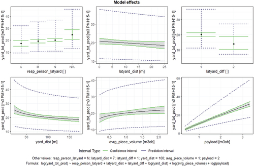
Figure 6. Model effect plot for model #7UB, with productive processing productivity (proc_prod_prod) as the response variable and payload (payload), average piece volume (avrg_piece_volume), and machine operator as predictors (resp_pers_yard_proc).

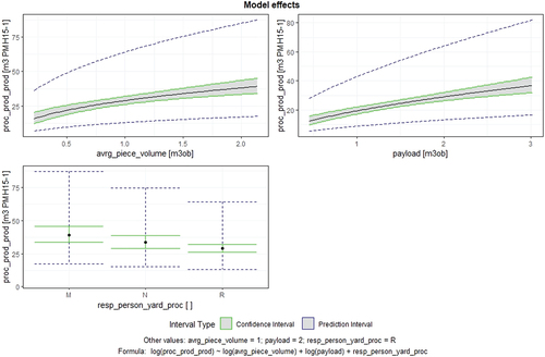
Figure 7. Model effect plot for model #9UB, with lateral yarding productivity (latyard_prod) as the response variable and the person responsible for carriage loading (resp_person_latyard), lateral yarding distance (latyard_dist), lateral yarding difficulty (latyard_diff), average piece volume (avrg_piece_volume) and payload (payload) as a predictor.

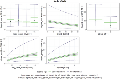
Table 11. Overview of model formulae recommended for predictive use, including the model coefficients. Variables are defined in Tables 3 and 4.

#	Model formula with coefficients	Remarks
1UB	yard_tot_prod = exp(β0–0.005657 latyard_dist −0.141275*log(yard_dist) + 0.141249*log(avrg_piece_volume) + 0.893245 * log(payload))	β0 = 3.020477 for latyard_diff == 1; β0 = 2.610445 for latyard_diff == 2
4All	yard_prod_prod = exp(β0–0.010459 latyard_dist − 0.200780 * log(yard_dist) + 0.199775 * log(avrg_piece_volume) + 0.793086 * log(payload))	β0 = 3.683075 for latyard_diff == 1; β0 = 3.352629 for latyard_diff == 2
6UB	proc_prod_prod = exp(2.96394 + 0.36392 * log(avrg_piece_volume) + 0.60480 * log(payload))
8All	latyard_prod = exp(β0–0.021793 * latyard_dist + 0.384590 * log(avrg_piece_volume) + 0.605868 * log(payload))	β0 = 3.737889 for latyard_diff == 1; β0 = 3.07891 for latyard_diff == 2

Figure A1. Model diagnostics plot (residual analysis plot) for model #5UB (unterlunkhofen and berikon sites); representative of all models.

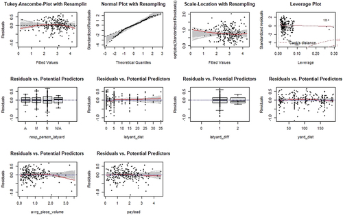
Table A1. Personnel and machine effort in the Muri study site.

Process		Staff/machine involved	Time (h)	Cost rate (CHF h^−1)	Total cost (CHF)
Felling	Staff	Very skilled workforce	19.00	99.00	1,881.00
		Trained workforce 1	58.50	80.00	4,680.00
		Worker in education	16.00	35.00	560.00
		Total staff	93.50		7,121.00
	Machines	Car [km]	70.00	1.00	70.00
		Forestry tractor (HSM)	11.50	120.00	1,380.00
		Forestry tractor (Deutz)	2.00	86.00	172.00
		Chainsaws	31.00	14.00	434.00
		Total machines			2,056.00
Installation	Staff	Planning	5.00	99.00	495.00
		Trained workforce 1	6.50	80.00	520.00
		External machine operator	6.50	94.00	611.00
		Machine operator	18.00	90.00	1,620.00
		Trained workforce 2	18.00	80.00	1,440.00
		Trained workforce 3	8.25	80.00	660.00
		Total staff	62.25		5,346.00
	Machines	Car [km]	10.00	1.00	10.00
		Car [km]	110.00	1.00	110.00
		Forestry tractor (HSM)	0.90	120.00	108.00
		Tractor (Valtliner)	0.90	120.00	108.00
		Excavator	6.50	120.00	780.00
		Koller K 507	11.00	230.00	2,530.00
		Total machines			3,646.00
Yarding	Staff	Machine operator	16.25	90.00	1,462.50
		Trained workforce 2	16.25	80.00	1,300.00
		Total staff	32.50		2,762.50
	Machines	Koller K 507	17.50	230.00	4,025.00
		Car [km]	110.00	1.00	110.00
		Total machines			4,135.00
Sorting	Staff	Trained workforce 1	13.75	80.00	1,100.00
and piling		Trained workforce 2	15.25	80.00	1,220.00
		Worker in education	9.00	35.00	315.00
		Total staff	38.00		2,635.00
	Machines	Forestry tractor (HSM)	18.50	80.00	1,480.00
		Chainsaws	12.00	14.00	168.00
		Total machines			1,648.00
Additional item	Lump sum	Street cleaning			700.00
Sum	Staff				17,864.50
	Machines				11,485.00
Resulting total cost (CHF)					30,049.50
Resulting relative cost (CHF m^−3)					102.14

Table A2. Personnel and machine effort in the Unterlunkhofen study site.

Process		Staff/machine involved	Time (h)	Cost rate (CHF h^−1)	Total cost (CHF)
Felling	Staff	Trained workforce 1	7.50	80.00	600.00
		Machine operator	7.50	90.00	675.00
		Total staff	15.00		1,275.00
	Machines	Car [km]	80.00	1.00	80.00
		Chainsaws	12.00	14.00	168.00
		Total machines			248.00
Installation	Staff	Planning	4.00	90.00	360.00
		Head enterprise	17.00	116.00	1,972.00
		Machine operator	7.75	90.00	697.50
		Trained workforce 1	12.00	80.00	960.00
		Trained workforce 2	7.75	80.00	620.00
		Trained workforce 3	5.00	80.00	400.00
		Total staff	53.50		5,009.50
	Machines	Car [km]	160.00	1.00	160.00
		Mounty MT 40–3	9.75	230.00	2,242.50
		Total machines			2,402.50
Yarding	Staff	Machine operator	6.25	90.00	562.50
		Trained workforce 1	6.25	80.00	500.00
		Trained workforce 2	6.25	80.00	500.00
		Head enterprise	1.25	116.00	145.00
		Total staff	20.00		1,707.50
	Machines	Mounty MT 40–3	7.25	230.00	1,667.50
		Car [km]	160.00	1.00	160.00
		Total machines			1,827.50
Sum	Staff		88.50		7,992.00
	Machines				4,478.00
Resulting total cost (CHF)					12,470.00
Resulting relative cost (CHF m^−3)					83.13

Table A3. Personnel and machine effort in the Berikon study site.

Process		Staff/machine involved	Time (h)	Cost rate (CHF h^−1)	Total cost (CHF)
Felling	Staff	Trained workforce 1	17.50	80.00	1,400.00
		Machine operator	17.50	90,00	1.575,00
		Total staff	35.00		2.975,00
	Machines	Car [km]	160.00	1,00	160,00
		Chainsaws	22.00	14,00	308,00
		Total machines			468,00
Installation	Staff	Planning	4.50	90,00	405,00
		Head enterprise	16.00	116,00	1.856,00
		Machine operator	7.50	90,00	675,00
		Trained workforce 1	23.50	80,00	1.880,00
		Trained workforce 2	16.00	80,00	1.280,00
		Total staff	67.50		6.096,00
	Machines	Car [km]	320.00	1,00	320,00
		Mounty MT 40–3	9.25	230,00	2.127,50
		Total machines			2.447,50
Yarding	Staff	Machine operator	9.50	90,00	855,00
		Trained workforce 1	33.50	80,00	2.680,00
		Trained workforce 2	9.50	80,00	760,00
		Head enterprise	24.00	116,00	2.784,00
		Total staff	76.50		7.079,00
	Machines	Mounty MT 40–3	30.75	230,00	7.072,50
		Car [km]	400.00	1,00	400,00
		Total machines			7.472,50
Sum	Staff		179.00		16.150,00
	Machines				10.388,00
Resulting total cost (CHF)					26,538.00
Resulting relative cost (CHF m^−3)					69.84

Varch T, Erber G, Visser R, Spinelli R, Harrill H, Stampfer K. 2021. Advances in cable yarding: a review of recent developments in skyline carriage technology. Curr For Rep. 7(4):181–194. doi: 10.1007/s40725-021-00150-x.

 Web of Science ®Google Scholar