Attractor landscapes: a unifying conceptual model for understanding behaviour change across scales of observation

Figures & data

Figure 1. Non-linear social change regarding mask wearing in Finland during the COVID-19 pandemic. In particular, the rapid shift from baseline values to greater uptakes, followed by oscillations, would not be described by linear or even piecewise linear regression. (Data source: Fan et al., 2020).

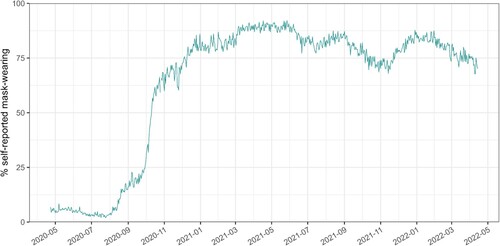
Figure 2. A conceptual basis to draw interpretations and stimulate multidisciplinary modelling. Configurations of variables (x₁, x₂ …) forming the system define its state space. In complex systems, this is often not flat (where every value is equally probable) but displays several equilibria, which depend on the value of extra parameters. Altogether, variables and parameters shape the state space V(x,p), which contains all equilibria. Parameters (p) here quantify the inter-relationships between variables, i.e., ‘how much’ a variable influences another. Stable equilibria – also known as attractors – are shown as valleys. To investigate how a system goes from one equilibrium to another, it is often sufficient to consider low-dimensional combinations of its variables (Kuehn et al., 2021) (extracted e.g., via principal component analysis, in which case the x₁ and x₂ would represent the two largest principal components, while the blue ridge identifies the main direction of change).

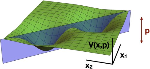
Figure 3. An attractor landscape with three different exemplifying states. Imagine the ball resembling the state of a person – e.g., location of ball in Panel A: ‘always takes precautions to mitigate contagion’, Panel B: ‘arbitrarily takes or does not take precautions’, and Panel C: ‘never takes precautions’. The two valleys represent stable (as defined by the local curvature below the ball) attractor states with different depths. Hence, the system is more prone to perturbations when in the rightmost attractor (Panel A) and more stable when in the leftmost attractor (Panel C). The transition from one attractor to the other happens when the system crosses the unstable ‘tipping point’ in the middle (Panel B). Arrows in Panels A and C represent the amount of variability we are likely to observe due to random perturbations on the system, a proxy for its stability. Lower stability translates into likely higher variability in the system’s state. Panel B also demonstrates that the landscape itself is not static but can change in the course of time (dashed line indicates the preceding landscape of panel A).

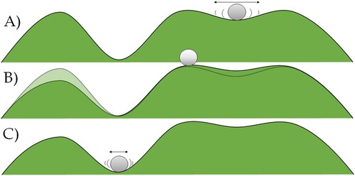
Figure 4. Two ways a system suddenly changes its state (i.e., two main types of critical transitions). B-tipping route (left): Due to an intervention or another learning or development process, the landscape itself changes, and when the state becomes unstable, the system ‘tips’ to the other attractor. N-tipping route (right): some exogenous perturbation, be it an intervention or a random event, jolts the ball over the threshold ‘hill’, where it stabilises in the new attractor.

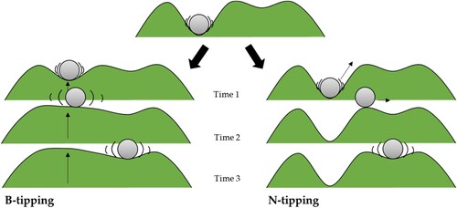
Figure 5. Demonstration of a society passing through several behavioural attractors during the COVID-19 pandemic. The underlying data are eight behavioural indicators collected daily in Finland (See text and supplementary website at https://heinonmatti.github.io/attractor-manuscript/ for details). Panel A: Reconstructing behavioural phases according to complex network approaches. Colours represent attractors for each day in the horizontal axis, with lighter colours indicating less precautions on average, and vice versa. The radius parameter defines a ‘detection threshold’ for the reconstruction of networks among the eight indicators; e.g., only the two most obvious attractors are observable on high radius values such as 0.25 (yellow area for lifting of restrictions despite community transmission of the Delta variant, and purple area for large-scale restrictions due to hospitalisations and deaths from both Delta and Omicron BA.1). Panel B: Raincloud plot of variables in the attractors, showing which values make up each regime at a representative radius (0.17), marked with a dashed line in Panel A. We can observe e.g., that each precaution is generally at its lowest during the yellow period, and highest in the purple period. As another example, we can also observe that people changed their shopping behaviour around the end of November, when the yellow regime ended. Panel C: Attractors reconstructed by Principal Component Analysis, as movement in the space of two main principal components (linear combinations of variables). The underlying conceptual model would correspond to Figure 2, but with four valleys instead of two. Colours to signify attractor types are imported from Panel B, at their corresponding temporal positions in Panel A, to illustrate convergence of the methods. The first principal component captures 68.4% of variance, and the second 20.3%.

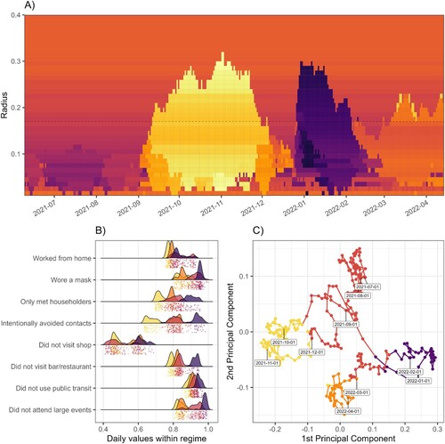
Table 1. A selection of features of complex systems, with examples to highlight relevance to behaviour change science. See also ‘The Visual Representation of Complexity’ (2018) and Table 1 in Heino et al. (2021).

Complexity concept, and how it occurs in attractor landscapes	Examples over two levels (individual behaviour change and group-level behaviour change)
Emergence: The interplay of micro-scale components gives rise to macro-scale patterns, which are not observable from a more limited scope or by a reductionist approach. In an attractor landscape, when you observe a system for a long time, you can also observe new ‘valleys’ emerging. Similar processes happen when the boundaries of the system under study are drawn differently (e.g., including not just adolescents in an intervention, but also their families, introduces social dynamics which did not exist in the smaller scope).	Individual level: Instances of an individual’s mask wearing behaviour gives rise to behavioural patterns (including automatic habits), which are not reducible to any particular instance of the behaviour, nor to a simple sum of all past behaviours. Group level: Individuals’ mask wearing behaviours contribute to the emergence of (patterns of) social norms, which are not reducible to any particular individual.
Feedback loops: The outcome of a process acts to further accelerate or dampen a change process, creating ‘vicious’ or ‘virtuous’ cycles. In an attractor landscape, feedbacks which act to oppose a change (such as ingrained habits) yield steeper ‘valleys’, that make the ball roll back to the bottom. Instead, accelerative feedbacks (such as intrinsic motivation propelled by success in changing a behaviour) can be thought of as pushing over the barriers, onto new attractors.	Individual level: Success in changing a behaviour increases a person’s intrinsic motivation to continue behaviour change efforts, further increasing the chances of success. Group level: In a public space where it is hard to keep a distance, people observe other people not keeping their distance, which leads to concluding that physical distancing is unimportant in the space, leading to fewer people physically distancing, and further reinforcing the crowdedness of the space.
Tipping points: A system can change little or not at all for a long time, until some threshold value is reached, and the system changes state radically in a relatively short period. In an attractor landscape, the system (i.e., the ‘ball’) reaches a ‘hilltop’ on the landscape and starts rolling to a new equilibrium.	Individual level: A person may hold persistent ambivalent attitudes and low intentions toward personal protective behaviours to mitigate contagion in the beginning of a pandemic. Stories of friends and family members getting seriously ill have seemingly little effect, until one day the person rapidly shifts their position. Group level: Support for an idea rapidly spreads beyond the initial vocal minority, after gaining sufficient salient acceptance in diverse social groups (e.g., ‘complex contagion’ processes in COVID-19 precautions; Centola, 2021).
Non-linearity: The outputs are not linearly proportional to the inputs, and large changes do not necessarily result from large events. In an attractor landscape, to leave a valley, a large change (jump) might result from large pushes from deep attractors, or from small pushes from de-stabilised states.	Individual level: Health promotion messages to change an attitude are unlikely to have the same impact on an individual when seen the first time, as compared to the 20th one, and changes in attitudes do not result in proportional changes in intention, yet alone behaviour. Group level: Consider a novel idea or a social representation. The speed of uptake increases or decreases depending on the current level of uptake, instead of remaining constant all the way through. See for example Figure 1; A single unit increase of time (x-axis), does not correspond to the same amount of increase in mask wearing (y-axis) throughout the period.
Sensitivity to initial conditions: Two systems which are almost identical, but differ in arbitrarily small quantities, can diverge wildly in their development as a response to an event (see Boeing, 2016 for an illustration). This implies fundamental problems to prediction, which additional data cannot solve in finite time. In an attractor landscape, a system close to b-tipping might jump or not, depending on whether it reaches its ‘critical mass’. Any small value below it does not yield to tipping.	Individual level: Two persons, having filled in identical survey answers (by which an intervention is tailored to them), can still react to the intervention in different and unpredictable manners. Also due to this, the trajectory of an N-of-1 time series can be unpredictable beyond a very short time horizon (e.g., 3–5 time points in Olthof, Hasselman, & Lichtwarck-Aschoff, 2020). Group level: Two intervention sites can depict very different reactions to an intervention, based on the social dynamics embedded in their history – hence necessitating local community involvement in the design of complex interventions.
Hysteresis: The effort required to enter a particular state may be very different from the effort required to exit it. In an attractor landscape, the adjacent possible state may be vastly deeper than the current one, or vice versa.	Individual level: A habit of consistent physical activity can take months to build, but days to break (i.e., switch back to an inactive state). Group level: The simple act of reinstating a mask mandate after its initial removal, does not necessarily result in equivalent compliance, as observed during the initial mandate.

Fan, J., Li, Y., Stewart, K., Kommareddy, A. R., Garcia, A., O’Brien, J., Bradford, A., Deng, X., Chiu, S., Kreuter, F., Barkay, N., Bilinski, A., Kim, B., Galili, T., Haimovich, D., LaRocca, S., Presser, S., Morris, K., Salomon, J. A., … Vannette, D. (2020). The University of Maryland Social Data Science Center Global COVID-19 Trends and Impact Survey, in partnership with Facebook. The Global COVID-19 Trends and Impact Survey Open Data API. https://covidmap.umd.edu/api.html.

 Google Scholar

Kuehn, C., & Bick, C. (2021). A universal route to explosive phenomena. Science Advances, 7(16), eabe3824. https://doi.org/10.1126/sciadv.abe3824

 PubMed Web of Science ®Google Scholar

Heino, M. T. J., Knittle, K., Noone, C., Hasselman, F., & Hankonen, N. (2021). Studying behaviour change mechanisms under complexity. Behavioral Sciences, 11(5), 77. https://doi.org/10.3390/bs11050077

 Web of Science ®Google Scholar

Centola, D. (2021). Complex contagions. In Research handbook on analytical sociology (1st ed., pp. 321–335). Edward Elgar Publishing. https://www.elgaronline.com/view/edcoll/9781789906844/9781789906844.00025.xml.

 Google Scholar

Boeing, G. (2016). Visual analysis of nonlinear dynamical systems: Chaos, fractals, self-similarity and the limits of prediction. Systems, 4(4), 37. https://doi.org/10.3390/systems4040037

 Web of Science ®Google Scholar

Olthof, M., Hasselman, F., & Lichtwarck-Aschoff, A. (2020). Complexity in psychological self-ratings: Implications for research and practice. BMC Medicine, 18(1), 317. https://doi.org/10.1186/s12916-020-01727-2

 PubMed Web of Science ®Google Scholar

Data availability statement

Data is available on the GitHub repository online: https://github.com/heinonmatti/attractor-manuscript.