Evaluating the reliability of bi-temporal canopy height model generated from airborne laser scanning for monitoring forest growth in boreal forest region

Figures & data

Figure 1. Flowchart of the data analysis methodology.

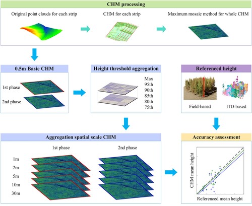
Figure 2. The study site is located in the Hulun Buir City, Inner Mongolia Autonomous Region, China. The coverage area is indicated by the red frame. It spans a distance of 5700 m from south to north and 5800 m from west to east.

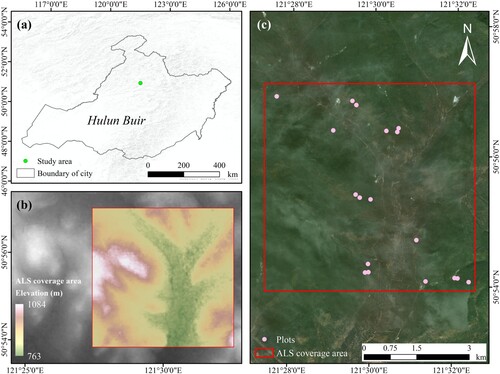
Table 1. The airborne laser scanning system parameters.

Species	Plot size (m^2)	number	DBH (cm)	Height (m)
Larix gmelinii	45 × 45	9	8.8 ± 37.7	9.1 ± 37.51
Betula platyphylla	45 × 45	2	10.5 ± 43.0	11.5 ± 22.3
Coniferous mixed forest	45 × 45	3	14.0 ± 43.0	12.6 ± 30.92
Coniferous and broad-leaved mixed forest	45 × 45	3	9.0 ± 31.1	8.15 ± 19.75

Note: x ± y, x is the median of the tree parameters for each tree species, y is the maximum value by which this parameter fluctuates up or down

Table 2. The airborne laser scanning system parameters.

ALS parameters	Acquisition time
	August 30th, 2012	August 28th, 2016
Aircraft	Yun-5	Yun-5
Flight speed	220 km/h	220 km/h
Flight altitude	2700 m	2200 m
Laser scanning sensor	Leica ALS60	Riegl LMS-Q680i
Wavelength	1064 nm	1550 nm
Laser pulse frequency	200 KHz	200 KHz
Average point density	5.6 pts/m^2	3.2 pts/m^2
Laser beam divergence	0.22 mrad	0.5 mrad
Scan angle	±35°	±30°

Table 3. The airborne CCD system parameters.

CCD parameters	Acquisition time
	August 30th, 2012	August 28th, 2016
CCD sensor	Leica RCD105	IGI DigiCAM-60
Wavelength	RGB	RGB
Resolution	0.5 m	0.5 m
Focal length	60 mm	50 mm
Field of view	55.3°	56.2°
Pixel size	6.8 μm	6 μm

Figure 3. Illustration of mosaic operators for maximum. In the overlapping area of the two raster datasets, each pixel is compared between the two rasters to determine the maximum value, which is then used as the value in the resulting mosaic.

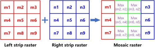
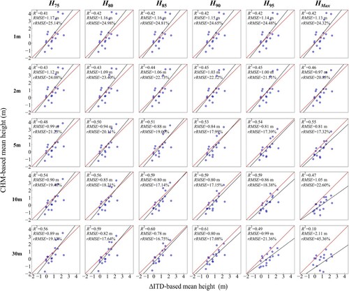
Figure 4. Based on different height metrics, comparison of CHM-based and field-based average height estimation results at different resolutions for 2012 and 2016.

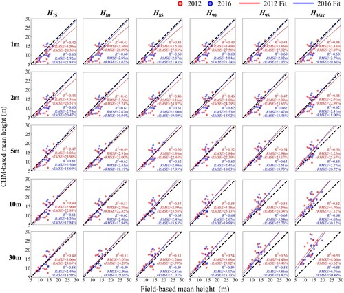
Figure 5. Based on different height metrics, comparison of CHM-based and ITS-based average height estimation results at different resolutions for 2012 and 2016.

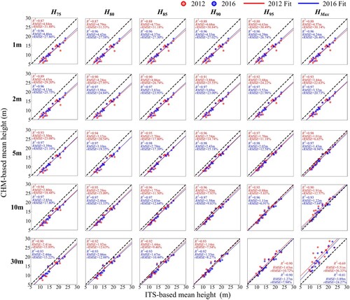
Figure 6. (a) and (b) represent the frequency distributions of canopy height for the years 2012 and 2016, respectively. (c) and (d) represent the CHMs for the years 2012 and 2016, respectively.

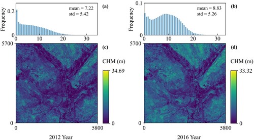
Figure 7. Based on different height metrics, the frequency distributions of CHMs at different resolutions for the years 2012 and 2016. The red and blue bars represent 2012 and 2016, respectively.

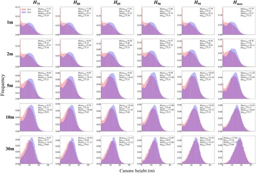
Figure 8. (a) Variation in canopy height across the entire study area by two 0.5 m CHMs. (b) The ΔCHM canopy height distribution. The dashed line represents zero value.

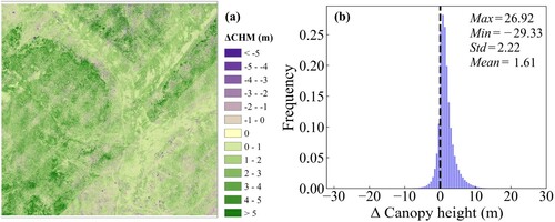
Figure 9. Histogram of difference canopy height frequency distributions based on six height percentile aggregation at five spatial scale. The dashed lines represent zero values.

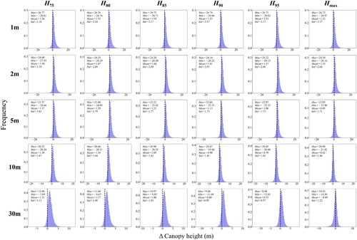
Table 4. Based on different height metrics, comparison of ΔCHM-based and Δfield-based arithmetic mean height estimation results at different resolutions.

Resolution (m)	Assessment Index	Height percentile
		H75	H80	H85	H90	H95	Hmax
1	R^2	0.0025	0.0025	0.0025	0.0024	0.0024	0.0024
	RMSE	1.95	1.94	1.93	1.93	1.92	1.91
	RRMSE	35.07%	34.95%	34.83%	34.71%	34.60%	34.48%
2	R^2	0.0020	0.0019	0.0019	0.0018	0.0017	0.0014
	RMSE	1.90	1.88	1.85	1.83	1.80	1.78
	RRMSE	34.28%	33.82%	33.36%	32.94%	32.50%	31.99%
5	R^2	0.0014	0.0010	0.0009	0.0005	0.0003	0.0007
	RMSE	1.81	1.76	1.71	1.64	1.59	1.54
	RRMSE	32.52%	31.61%	30.72%	29.62%	28.65%	27.74%
10	R^2	0.0003	0.0001	0.0000	0.0000	0.0017	0.0046
	RMSE	1.73	1.67	1.60	1.55	1.50	1.52
	RRMSE	31.11%	30.04%	28.85%	27.96%	27.07%	27.40%
30	R^2	0.0004	0.0024	0.0047	0.0094	0.0076	0.0198
	RMSE	1.70	1.60	1.52	1.44	1.49	2.47
	RRMSE	30.55%	28.83%	27.29%	25.97%	26.83%	44.50%

Table 5. Based on different height metrics, comparison of ΔCHM-based and ΔITS-based arithmetic mean height estimation results at different resolutions.

Resolution (m)	Assessment Index	Height percentile
		H75	H80	H85	H75	H95	max
1	R^2	0.41	0.42	0.42	0.42	0.42	0.42
	RMSE	1.17	1.16	1.16	1.15	1.14	1.13
	RRMSE	25.14%	24.98%	24.81%	24.65%	24.48%	24.32%
2	R^2	0.43	0.43	0.44	0.45	0.45	0.46
	RMSE	1.12	1.09	1.06	1.03	1.00	0.97
	RRMSE	24.08%	23.40%	22.73%	22.12%	21.51%	20.85%
5	R^2	0.48	0.50	0.51	0.53	0.54	0.55
	RMSE	0.99	0.94	0.88	0.84	0.81	0.81
	RRMSE	21.23%	20.11%	19.00%	17.99%	17.39%	17.32%
10	R^2	0.54	0.56	0.59	0.59	0.59	0.47
	RMSE	0.90	0.85	0.80	0.80	0.86	1.05
	RRMSE	19.40%	18.21%	17.14%	17.15%	18.38%	22.60%
30	R^2	0.56	0.59	0.60	0.61	0.49	0.10
	RMSE	0.89	0.82	0.78	0.80	0.99	2.11
	RRMSE	19.13%	17.64%	16.75%	17.08%	21.36%	45.36%

Table 6. Statistical parameters of mean values at different resolutions and height percentiles of the CHM raster corresponding to the data from the two sample periods.

Height percentile	Resolution (m)	Number of samples	Mean (m)	Standard deviation (m)	Standard error of mean (m)	Variance (m^2)
H75	1	34	11.10	3.84	0.66	14.71
H75	2	34	11.46	3.87	0.66	14.97
H75	5	34	12.27	4.01	0.69	16.04
H75	10	34	12.91	4.02	0.69	16.12
H75	30	34	13.47	4.04	0.69	16.31
H80	1	34	11.15	3.84	0.66	14.73
H80	2	34	11.63	3.88	0.67	15.08
H80	5	34	12.60	4.02	0.69	16.13
H80	10	34	13.37	4.04	0.69	16.29
H80	30	34	13.95	4.03	0.69	16.25
H85	1	34	11.19	3.84	0.66	14.75
H85	2	34	11.79	3.89	0.67	15.10
H85	5	34	12.96	4.02	0.69	16.18
H85	10	34	13.87	4.06	0.70	16.47
H85	30	34	14.50	4.03	0.69	16.28
H90	1	34	11.24	3.84	0.66	14.78
H90	2	34	11.95	3.89	0.67	15.15
H90	5	34	13.37	4.04	0.69	16.29
H90	10	34	14.44	4.06	0.70	16.48
H90	30	34	15.18	4.07	0.70	16.60
H95	1	34	11.29	3.85	0.66	14.80
H95	2	34	12.13	3.90	0.67	15.23
H95	5	34	13.86	4.05	0.70	16.44
H95	10	34	15.19	4.06	0.70	16.51
H95	30	34	16.16	4.22	0.72	17.81
Hmax	1	34	11.34	3.85	0.66	14.82
Hmax	2	34	12.34	3.91	0.67	15.32
Hmax	5	34	14.58	4.09	0.70	16.77
Hmax	10	34	16.59	4.13	0.71	17.03
Hmax	30	34	19.64	4.88	0.84	23.83

Table 7. ANOVA statistic of the effect of spatial resolution and height percentile on the CHM at the 0.05 significance level.

	ANOVA components	Degree of freedom	Mean square	F statistic	F probability
Height percentile	Model	5	156.41	8.36	0.00
	Error	1014	18.71
	Total	1019
Resolution	Model	4	626.59	36.87	0.00
	Error	1015	16.99
	Total	1019
Two-way	Height percentile	5	156.41	9.71	0.00
	Resolution	4	626.59	38.90	0.00
	Interaction	20	25.95	1.61	0.04
	Model	29	131.29	8.15	0.00
	Error	990	16.11
	Total	1019

Figure 10. Five sampling strips comparing the consistency of ΔCHM generated by the two strategies. (a) Conventional method-derived 0.5 m ΔCHM. (b) Proposed method-derived 0.5 m ΔCHM. (c) Comparison of ΔCHM profiles for 5 sampling strips.

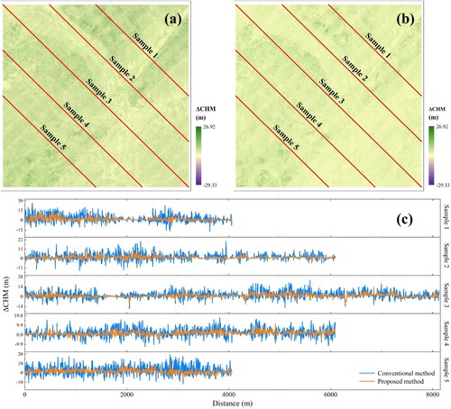
Figure 11. (a) The mean height of field-based in plots in 2012 and 2016. (b) The mean height of ITS-based in plots in 2012 and 2016. (c) The max height of LiDAR-derived in plots in 2012 and 2016. (d) (e) The highlighted plot in (a) (b) (c) corresponds to the CHM in 2012 and 2016. (f) The highlighted plot corresponds to the point cloud in 2012 and 2016, three representative sub-regions were selected in (i) (ii) (iii).

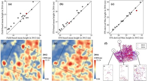
Figure 12. Four representative sub-regions to explore the possible factors of canopy height change in the study area. (i) and (ii) are CHM in 2012 and 2016; (iii) and (iv) are CCD images in 2012 and 2016; (v) and (vi) are point cloud height profiles in 2012 and 2016; (vii) is CHM height frequency distribution statistics, the red line and blue line respectively represent 2012 and 2016. (a) indicates the presence of logging; (b) indicates less growth; (c) indicates forest road development; (d) indicates more growth.

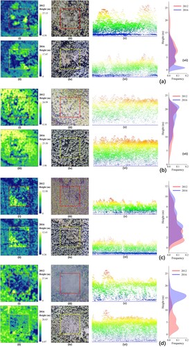
Figure A1. (a) and (b) are the fitted growth curves of Larix gmelinii and Betula platyphylla respectively. We established Schumacher growth functions of Larix gmelinii and Betula platyphylla using the tree age and tree height sampling data from the dataset. Based on the theoretical application of the Schumacher growth function (Burkhart and Tomé 2012).

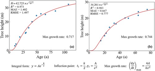
Figure A2. The high resolution figure of Figure 4.

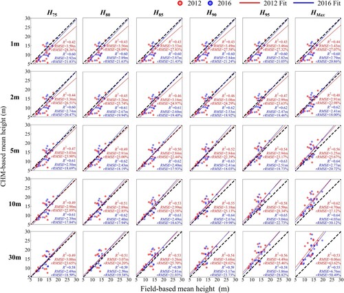
Figure A3. The high resolution figure of Figure 5.

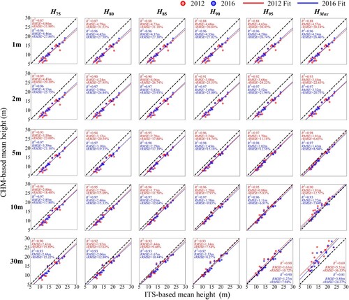
Figure A4. The scatter plot corresponding to Table 4. Based on different height metrics, comparison of ΔCHM-based and Δfield-based arithmetic mean height estimation results at different resolutions.

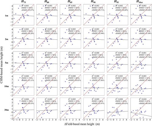
Figure A5. The scatter plot corresponding to Table 5. Based on different height metrics, comparison of ΔCHM-based and ΔITS-based arithmetic mean height estimation results at different resolutions.

Burkhart, Harold E., and Margarida Tomé. 2012. Modeling Forest Trees and Stands. Dordrecht: Springer Netherlands. https://doi.org/10.1007/978-90-481-3170-9

 Google Scholar