Calibration and validation of high frequency coastal radar waves exploiting in-situ observations and modelled data in the south-west Sicily

Figures & data

Figure 1. (a) Map of the area with the main circulation features: Atlantic current (AC), Atlantic Ionian Stream (AIS) and Tunisian Atlantic Current (ATC). The red rectangle indicates the studied area enlarged in (b), where the percentage of HFR data coverage from 1/4/21–31/031/22 is depicted. Mazara del Vallo ondametric buoy (red triangle) and WERA HFR position (blue triangle) are indicated. The area in green encloses the HFR grid points (blue points) considered in the analysis; the sector delimited by red lines corresponds to sFOV.

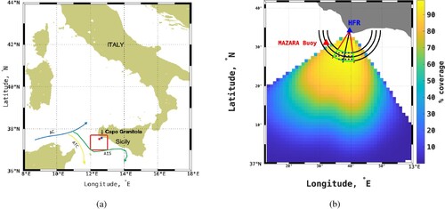
Figure 2. (a) Directional distribution of significant wave heights measured by ondametric buoy. (b) Studied area with model grid points (red), radar grid points (blue) and superimposed bathymetry (from EMODNET, https://www.emodnet-bathymetry.eu/). The area in green contains the HFR points (blue stars numbered) where data have been considered for the comparison with buoy timeseries and for the correlation calculations with model points (red circles). Sector delimited by red lines corresponds to sFOV. (c) distribution of wavelengths λ measured from Mazara del Vallo Buoy (red triangle) in the period April 2021 - March 2022.

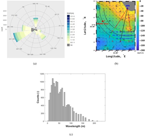
Figure 3. Correlation coefficient between Hm0_HFR,unc at stars within the green-bordered area and Hm0_buoy. Green star corresponds to the location P3 where HFR data have been considered for optimisation and validation.

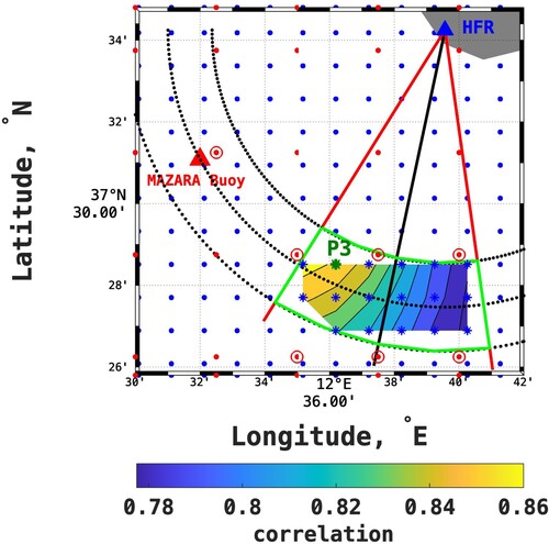
Figure 4. (a) Time series of Hm0_HFR,unc, Hm0_buoy, Hm0_CMS-buoy, Hm0_CMS-P3, obtained: from buoy (blue line), from HFR at P3 (black line) and from model data both at buoy location (green line) and close to P3 (red line). (b) zoom of (a) for the period 20/11/21–15/12/21. (c) zoom of (a) for the period 1/02/22–28/02/22. The dashed line indicates the noise threshold.

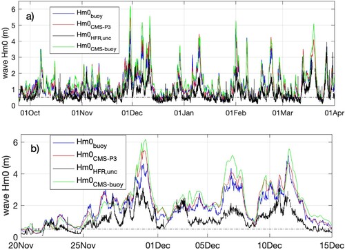
Figure 5. Scatter plot of: (a) Hm0_HFR,unc at P3 versus Hm0 from buoy, and (b) Hm0 from model at P3 versus Hm0 from buoy for the period 1/4/2021–31/3/2022. Linear fit coefficients are indicated.

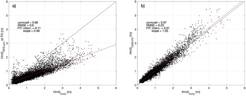
Table 1. Correlations (R), RMSE and bias among all timeseries at 95% confidence level for the period 1/4/2021–31/3/2022.

	Hm0CMS-P3	Hm0CMS-buoy	Hm0 buoy	Hm0HFR,unc
Hm0CMS-P3	-
Hm0CMS-buoy	R = 0.96 RMSE = 0.25 m bias = 0.08 m	-
Hm0buoy	R = 0.97 RMSE = 0.20 m bias = −0.04 m	R = 0.93 RMSE = 0.32 m bias = −0.11 m	-
Hm0HFR,unc	R = 0.86 RMSE = 0.67 m bias = −0.48 m	R = 0.81 RMSE = 0.78 m bias = −0.55 m	R = 0.86 RMSE = 0.60 m bias = −0.43 m	-

Figure 6. (a) Correlation between reference Hm0 (from model at P3 grid point) and HFR second power spectra at each of the 21 frequencies, before optimisation. (b) Optimised α parameters obtained by means of least squares-constrained fitting using Hm0_CMS-P3 as reference data (purple line) and original alpha set (yellow line). (c) Optimised Hm0_HFR vs Hm0_CMS and (d) validated Hm0_HFR vs Hm0_CMS (e) Correlation between reference Hm0 (from buoy) and HFR second power spectra at each of the 21 frequencies, before optimisation. (f) Optimised α parameters obtained by means of least squares-constrained fitting using Hm0_buoy as reference data (purple line) and original alpha set (yellow line). (g) Optimised Hm0_HFR vs Hm0_buoy and (h) validated Hm0_HFR vs Hm0_buoy.

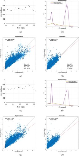
Table 2. Correlation coefficients, RMSE, bias and coefficients (slope and intercept) of linear regression before optimisation and after it for both periods D1 and D2, with Hm0_CMS and Hm0_buoy as references.

Period	Sub-range	#points		corr		RMSE		bias
		Model	Buoy	Model	Buoy	Model	Buoy	Model	Buoy
D2	before optimisation	13775	13844	0.86	0.87	0.85	0.76	0.67	0.62
	after constr. optim.			0.87	0.88	0.44	0.37	−0.07	−0.02
D1	before validation	9981	9982	0.80	0.83	0.50	0.47	0.40	0.35
	after constr. valid.			0.79	0.82	0.41	0.36	−0.19	−0.16

Figure 7. Time series of Hm0 from buoy and from radar, both uncalibrated and optimised, for period D1 (a) and D2 (b). Time series has been split into two panels and a 7-points moving average has been applied to Hm0_HFR for readability (pay attention that the vertical scale is not the same in the two panels).

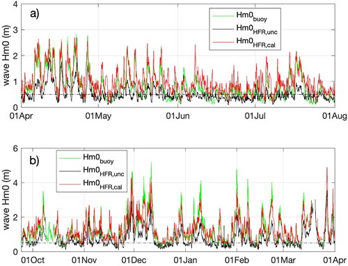
Figure 8. (a) Scatter plot of calibrated Hm0_HFR at P3 versus Hm0_buoy for the complete period considered; the outliers are indicated in red. (b) zoom of the Hm0_buoy and Hm0_HFR,unc timeseries for the period 5/4/21–3/5/21 with the outliers in (a) marked as red points.

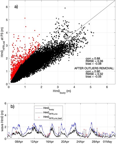
Table 3. Correlation coefficients and RMSE between Hm0 from radar and from buoy, calculated over the entire dataset, before and after optimisation, considering different ranges for Hm0.

	Hm0HFR,unc - Hm0buoy		Hm0HFR,cal - Hm0buoy
	R	RMSE (m)	R	RMSE (m)
0.5 m ≤ Hm0 < 1.3 m	0.61	0.40	0.62	0.30
1.3 m ≤ Hm0 < 2 m	0.41	0.78	0.42	0.37
Hm0 ≥ 2 m	0.61	1.30	0.67	0.53