1,005
Views
3
CrossRef citations to date
0
Altmetric
Research Article

A dynamic closure modeling framework for large eddy simulation using approximate deconvolution: Burgers equation

& ORCID Icon |
Article: 1464368 | Received 28 Jul 2017, Accepted 06 Apr 2018, Published online: 27 Apr 2018

Figures & data

Figure 1. Transfer functions of the sixth-order compact Padé filters for various free filtering parameters.
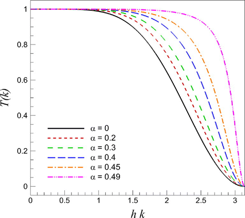
Figure 1. Transfer functions of the sixth-order compact Padé filters for various free filtering parameters.

Figure 2. Conservative formulation results for solving the Burgers equation initiated by the single-mode sine wave: (a) time evolution by DNS with resolution of N=32768; (b) under-resolved numerical simulation (UNS); (c) dynamic Smagorinsky model (D-SMA); and (d–f) the proposed dynamic AD model (D-AD) with various orders of Q. In (b–f), we present the final snapshots at time t=2.5 using resolutions of 512, 1024, and 2048 where the results for 512 and 1024 resolutions are shifted in the x-axis for the purpose of illustration.
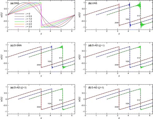
Figure 2. Conservative formulation results for solving the Burgers equation initiated by the single-mode sine wave: (a) time evolution by DNS with resolution of N=32768; (b) under-resolved numerical simulation (UNS); (c) dynamic Smagorinsky model (D-SMA); and (d–f) the proposed dynamic AD model (D-AD) with various orders of Q. In (b–f), we present the final snapshots at time t=2.5 using resolutions of 512, 1024, and 2048 where the results for 512 and 1024 resolutions are shifted in the x-axis for the purpose of illustration.

Figure 3. Conservative formulation for the shock formation problem initiated by a single-mode sine wave using 512 grid points: a comparison for the time evolution of the dissipation rate (left) and its close-up for local enlargement (right).
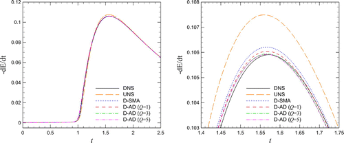
Figure 3. Conservative formulation for the shock formation problem initiated by a single-mode sine wave using 512 grid points: a comparison for the time evolution of the dissipation rate (left) and its close-up for local enlargement (right).

Figure 4. Skew-symmetric formulation simulation results for solving the Burgers equation initiated by the single-mode sine wave: (a) time evolution by DNS with resolution of N=32768; (b) under-resolved numerical simulation (UNS); (c) dynamic Smagorinsky model (D-SMA); and (d–f) the proposed dynamic AD model (D-AD) with various orders of Q. In (b–f), we present the final snapshots at time t=2.5 using resolutions of 512, 1024, and 2048 where the results for 512 and 1024 resolutions are shifted in the x-axis for the purpose of illustration.
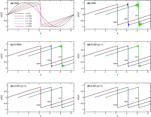
Figure 4. Skew-symmetric formulation simulation results for solving the Burgers equation initiated by the single-mode sine wave: (a) time evolution by DNS with resolution of N=32768; (b) under-resolved numerical simulation (UNS); (c) dynamic Smagorinsky model (D-SMA); and (d–f) the proposed dynamic AD model (D-AD) with various orders of Q. In (b–f), we present the final snapshots at time t=2.5 using resolutions of 512, 1024, and 2048 where the results for 512 and 1024 resolutions are shifted in the x-axis for the purpose of illustration.

Figure 5. Skew-symmetric formulation for the shock formation problem initiated by a single-mode sine wave using 512 grid points: a comparison for the time evolution of the dissipation rate (left) and its close-up for local enlargement (right).
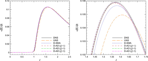
Figure 5. Skew-symmetric formulation for the shock formation problem initiated by a single-mode sine wave using 512 grid points: a comparison for the time evolution of the dissipation rate (left) and its close-up for local enlargement (right).

Figure 6. A comparison of energy spectra for N=512 resolution results at time t=2.5 obtained by the conservative (left) and skew-symmetric (right) formulations for the shock formation problem initiated by a single-mode sine wave.
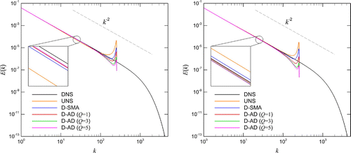
Figure 6. A comparison of energy spectra for N=512 resolution results at time t=2.5 obtained by the conservative (left) and skew-symmetric (right) formulations for the shock formation problem initiated by a single-mode sine wave.

Figure 7. Intercomparison of N=512 resolution results for solving the Burgers equation initiated by the single-mode sine wave using the conservative formulation (left column) and the skew-symmetric formulation (right column). Note that the simulation results for UNS, D-SMA, D-AD (Q=3), and D-AD (Q=5) are shifted in x-axis for the purpose of illustration.
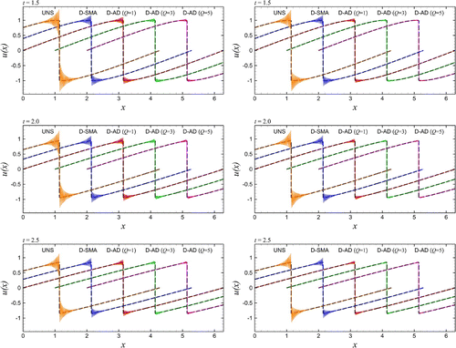
Figure 7. Intercomparison of N=512 resolution results for solving the Burgers equation initiated by the single-mode sine wave using the conservative formulation (left column) and the skew-symmetric formulation (right column). Note that the simulation results for UNS, D-SMA, D-AD (Q=3), and D-AD (Q=5) are shifted in x-axis for the purpose of illustration.

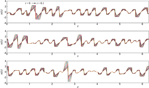
Figure 8. Space–time solutions of the Burgers equation using three different initial conditions generated from Equation (Equation40).

Figure 8. Space–time solutions of the Burgers equation using three different initial conditions generated from Equation (Equation40(40) E(k)=23πk4k05e-(k/k0)2,(40) ).

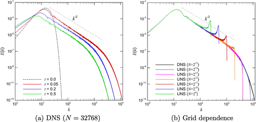
Figure 9. Time evolution of the energy spectrum for the Burgers turbulence problem based upon the ensemble average of 64 sample fields obtained by DNS (N=32768) (left), and a comparison of energy spectra at time t=0.05 obtained by various spatial resolutions ranging from N=512 to N=32768 (right).

Figure 9. Time evolution of the energy spectrum for the Burgers turbulence problem based upon the ensemble average of 64 sample fields obtained by DNS (N=32768) (left), and a comparison of energy spectra at time t=0.05 obtained by various spatial resolutions ranging from N=512 to N=32768 (right).

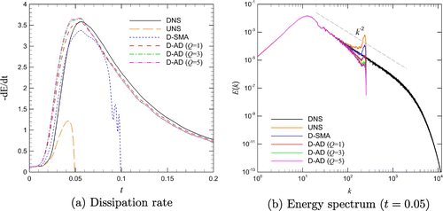
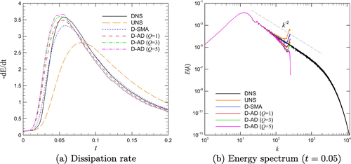
Figure 10. Results for the SGS modeling of the Burgers turbulence problem obtained using N=512 resolution with the conservative formulation of the nonlinear term: time evolution of the total dissipation rate (left) and energy spectra at time t=0.05 (right).

Figure 10. Results for the SGS modeling of the Burgers turbulence problem obtained using N=512 resolution with the conservative formulation of the nonlinear term: time evolution of the total dissipation rate (left) and energy spectra at time t=0.05 (right).

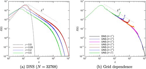
Figure 11. Time evolution of the energy spectrum for the Burgers turbulence problem based upon the ensemble average of 64 sample fields obtained by DNS (N=32768) (left), and energy spectra at time t=0.05 obtained by various spatial resolutions ranging from N=512 to N=32768 (right).

Figure 11. Time evolution of the energy spectrum for the Burgers turbulence problem based upon the ensemble average of 64 sample fields obtained by DNS (N=32768) (left), and energy spectra at time t=0.05 obtained by various spatial resolutions ranging from N=512 to N=32768 (right).

Figure 12. Results for the SGS modeling of the Burgers turbulence problem obtained using N=512 resolution with the skew-symmetric formulation of the nonlinear term: time evolution of the total dissipation rate (left) and energy spectra at time t=0.05 (right).

Figure 12. Results for the SGS modeling of the Burgers turbulence problem obtained using N=512 resolution with the skew-symmetric formulation of the nonlinear term: time evolution of the total dissipation rate (left) and energy spectra at time t=0.05 (right).

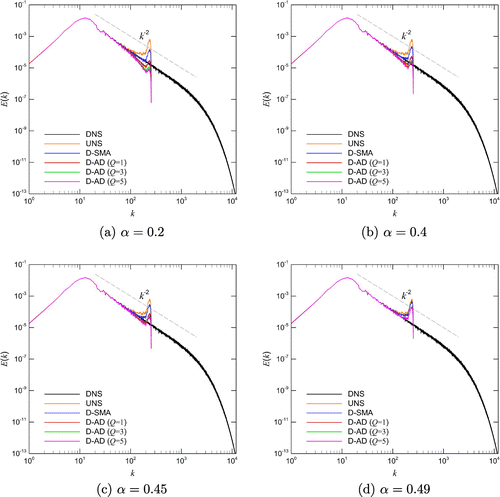
Figure 13. A sensitivity analysis with respect to the free filtering parameter α for solving the Burgers turbulence problem and showing the energy spectra at time t=0.05 using the conservative formulation on N=512 resolution.

Figure 13. A sensitivity analysis with respect to the free filtering parameter α for solving the Burgers turbulence problem and showing the energy spectra at time t=0.05 using the conservative formulation on N=512 resolution.

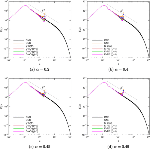
Figure 14. A sensitivity analysis with respect to the free filtering parameter α for solving the Burgers turbulence problem and showing the energy spectra at time t=0.05 using the skew-symmetric formulation on N=512 resolution.

Figure 14. A sensitivity analysis with respect to the free filtering parameter α for solving the Burgers turbulence problem and showing the energy spectra at time t=0.05 using the skew-symmetric formulation on N=512 resolution.