Energy-Dependent, Self-Adaptive Mesh h(p)-Refinement of an Interior-Penalty Scheme for a Discontinuous Galerkin Isogeometric Analysis Spatial Discretization of the Multi-Group Neutron Diffusion Equation with Dual-Weighted Residual Error Measures

Figures & data

Figure 1. An example of a 2D pin-cell represented by bi-quadratic NURBS patches (macro-elements) in the real physical space, $V,$ as denoted by the parameters x and y (Wilson, Eaton, and Kópházi 2024). The domain, represented in the parametric space, $\widehat{V},$ is formed from the tensor-product of two 1D spaces, as denoted by the parameters $\widehat{\xi }$ and $\widehat{\eta }.$ The parametric space has been decomposed into non-vanishing knot-spans (micro-elements), over which, numerical integration is performed by an affine mapping from the parent domain, $\tilde{V},$ as denoted by the parameters $\tilde{\xi }$ and $\tilde{\eta }.$ The patch boundaries are highlighted in red; whereas the non-vanishing knot-spans within a patch are separated by black lines. The image of given non-vanishing knot-span, shaded in dark grey, can be represented in all three spaces. (V. the web-based version for reference to color.).

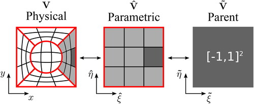
Figure 2. The Jacobian determinant for the example of a 2D unit circle as represented by a single degenerate bi-quadratic NURBS patch (left) and five non-degenerate bi-quadratic NURBS patches (right). The geometrical mapping is non-invertible at the corners of the circle on the left-hand side where the Jacobian determinant becomes negligibly small. (V. the web-based version for reference to color.).

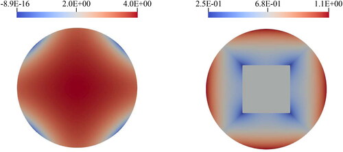
Figure 3. The left and right-hand sides are the result of inserting knots at $\xi \text{=}0.5$ with multiplicity $\dot{m}=p,p+1,$ respectively, into a basis of quadratic ($p\text{=}2$) B-splines with no initial internal refinement structure; i.e.,, ${\Xi }_{\xi }\text{=}\{0,0,0,1,1,1\}.$ In either case, continuity in the basis has been reduced enough to form a new patch boundary, $\partial {\widehat{V}}_{12},$ and the parametric space has been renormalized to $[0,1]$ in each of the newly formed patches, ${\widehat{V}}_1$ and ${\widehat{V}}_2.$ C⁰-continuity across $\partial {\widehat{V}}_{12}$ is naturally enforced in a strong sense for $\dot{m}\text{=}p;$ however, the basis becomes discontinuous, or $C^{‐1}$-continuous across $\partial {\widehat{V}}_{12}$ for $\dot{m}\text{=}p+1,$ where it must be explicitly enforced in either a strong sense or a weak one. (V. the web-based version for reference to color.).

Figure 4. A comparison between the solutions (right) of an SIP-DG-IGA discretization and its CBG-IGA counterpart along the line at $y=‐1.00$ over an irregular mesh (left) for the example of a simple problem; a one-speed, ($2\text{cm}\times 2\text{cm}$) homogeneous bare-square with isotropic unit-source, ${\Sigma }_t=1.00{\text{cm}}^{‐1},$ c = 0.7. Across 52 bilinear patches, strict C⁰-continuity enforced in the CBG discretization (73 DoFs), whilst this is relaxed in the DG discretization (208 DoFs). (V. the web-based version for reference to color.).

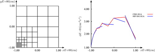
Figure 5. For the example of a 2D unit pin-cell mesh of 13 non-degenerate bi-quadratic NURBS patches (left), a comparison is made between those TICs, $C_{e,f}^{\mathit{\text{lit}}},C_{e,f}^0$ and $C_{e,f}^1,$ as calculated from the literature, Equation 69(69) $$C_{e,f}^{\mathit{\text{lit}}}={(p+1)}^2\frac{A(\partial V_f)}{V(V_e)}\text{;}$$(69) , the mass matrix method, Equation 66a(66a) $$\Vert {\gamma }_0\widehat{u}{\Vert }_{L_2(\partial V_e)}^2\le C_{e,f}^0\Vert \widehat{u}{\Vert }_{L_2(V_e)}^2\text{;}$$(66a) , and the stiffness matrix method, Equation 66b(66b) $$\Vert {\gamma }_1\widehat{u}{\Vert }_{L_2(\partial V_e)}^2\le C_{e,f}^1\Vert \overrightarrow{\nabla }\widehat{u}{\Vert }_{L_2(V_e)}^2.$$(66b) , respectively. The ten distinct faces are labeled 1 through 10; and all TIC values are normalized by $\times V(V_e)/A\partial V_f.$ The distinction between Faces $\partial V_{7a}$ and $\partial V_{7b}$ is such that the former is the the single distinct face of the central (red) circle constructed from a single degenerate NURBS patch; whereas the latter belongs to the set of distinct faces that belong to the central circle as it is presented, constructed from five non-degenerate NURBS patches. Those TIC values that are invariant with any change to the radii are presented in the table (right). (V. the web-based version for reference to color.).

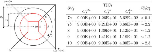
Figure 6. A parametric study that compares TIC values for the distinct Faces $\partial V_1$ (top left), $\partial V_2$ (top right), $\partial V_3$ (middle left), $\partial V_4$ (middle right), $\partial V_5$ (bottom left), and $\partial V_6$ (bottom right) of a 2D unit pin-cell mesh as the outer-radius is varied; v. Figure 5. In each instance, the volume patch and the face patches may be defined by $r_o,$ which is varied between 0.05 and 0.45 cm. In the case of $\partial V_4,\partial V_5$ and $\partial V_6,r_i$ is fixed at 0.025 cm. (V. the web-based version for reference to color.).

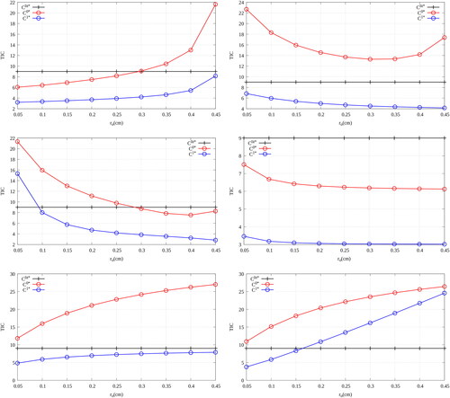
Figure 7. A parametric study that compares TICs for the distinct Faces $\partial V_{7a}$ (left) and $\partial V_{7b}$ (right) of a 2D unit pin-cell mesh as the number of quadrature points is varied; v. Figure 5. In each instance, the TICs are invariant with any change to the radii. (V. the web-based version for reference to color.).

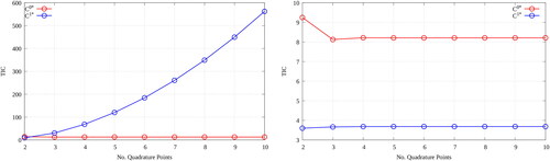
Figure 8. A parametric study of the $H^1$-error (right) and the spectral conditioning (right) of the SIP-DG-IGA discretization of the 1G NDE for the example of a 2D unit pin-cell mesh; qq.v. Table 1 and Section 6.1.2. The penalty parameters of each face are varied as ${\mu }_f^{*}=\alpha \times {\mu }_f.$ (V. the web-based version for reference to color.).

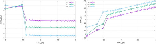
Table 1. The nuclear data for the 2D 1G MMS verification.

Material	g	D^g(cm)	${\Sigma }_t^g$ (^−1)	${\Sigma }_{s0}^{g\to 1}$ (cm ^−1)
(1)	1	$3.333\mathrm{E}-01$	$1.000\mathrm{E}+00$	$5.000\mathrm{E}-01$

Figure 9. The convergence plots, ${ϵ}_{H^1}$v h (left) and ${ϵ}_{H^1}$v DoFs (right), for the MMS verification of the uniform refinement of the SIP-DG-IGA 1G NDE over a 2D Cartesian mesh. The manufactured solution is chosen as per Equation 76 for n = 0 (top row), n = 1 (middle row) and n = 2 (bottom row). (V. the web-based version for reference to color.).

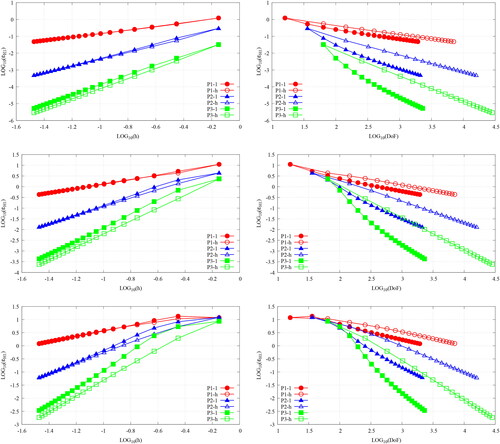
Table 2. The asymptotic orders of accuracy, Equations 74, for the MMS verification of the uniform refinement of the SIP-DG-IGA 1G NDE over a 2D Cartesian mesh.

		KI-1		KI-h
	p	${ϵ}_{H^1}$	${ϵ}_{L_2}$	${ϵ}_{H^1}$	${ϵ}_{L_2}$
(n = 0)	1	1.00	2.00	1.00	2.00
	2	2.05	3.03	2.00	2.99
	3	2.98	3.98	3.00	4.00
(n = 1)	1	1.00	2.01	1.02	1.98
	2	2.06	3.05	2.00	3.00
	3	3.01	4.03	3.00	3.99
(n = 2)	1	1.00	2.01	1.04	1.96
	2	2.08	3.09	2.01	3.01
	3	3.06	4.09	3.01	3.98

The convergence rates are evaluated as the slope of the last few points from each dataset.

Figure 10. The convergence plots, ${ϵ}_{H^1}$v DoFs, for the MMS verification of the NRG-AMR-h(p) of the SIP-DG-IGA 1G NDE over a 2D Cartesian mesh. The manufactured solution is chosen as per Equation 76 for n = 0 (top left), n = 1 (top right) and n = 2 (bottom). (V. the web-based version for reference to color.).

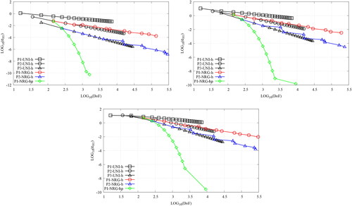
Table 3. The nuclear data for the 2D 2G MMS verification.

Material	g	D^g (cm)	${\Sigma }_t^g$ (cm ^−1)	${\Sigma }_{s0}^{g\to 1}$ (cm^−1)	${\Sigma }_s^{g\to 2}$ (cm^−1)
(1) -	1	3.333E − 01	1.000E − 01	5.000E − 01	2.500E − 01
(1) -	2	3.333E − 01	1.000E − 01	0.000E − 01	5.000E − 01

Figure 11. The convergence plots, ${ϵ}_{H^1}$v h (left) and ${ϵ}_{H^1}$v DoFs (right), for the MMS verification of the uniform refinement of the SIP-DG-IGA 2G NDE over a 2D pin-cell mesh. The manufactured solutions are chosen as per Equation 77 for g = 1, 2. (V. the web-based version for reference to color.).

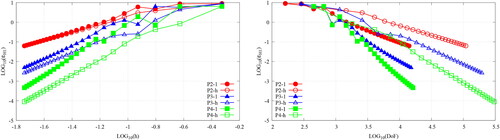
Table 4. The asymptotic orders of accuracy, Equations 74, for the MMS verification of the uniform refinement of the SIP-DG-IGA 2G NDE over a 2D pin-cell mesh.

	KI-1		KI-h
P	${ϵ}_{H^1}$	${ϵ}_{L_2}$	${ϵ}_{H^1}$	${ϵ}_{L_2}$
2	2.06	3.15	2.00	3.03
3	3.09	4.18	3.00	3.97
4	4.29	5.40	3.99	5.02

The convergence rates are evaluated as the slope of the last few points from each dataset.

Figure 12. The convergence plots, ${ϵ}_{H^1}$v DoFs, for the MMS verification of the NRG-AMR-h(p) of the SIP-DG-IGA 2G NDE over a 2D pin-cell mesh. The prefixes M1- and M2- denote the use of energy-independent and energy-dependent meshes, respectively. The manufactured solutions are chosen as per Equation 77 for g = 1, 2. (V. the web-based version for reference to color.).

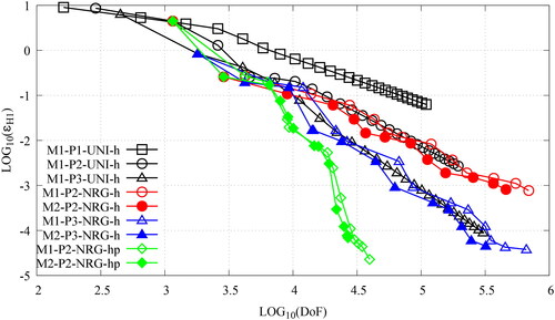
Figure 13. The plots of the effectivity index, ${\theta }_{H^1}$v DoFs, for the MMS verification of the NRG-AMR-h(p) of the SIP-DG-IGA 2G NDE over a 2D pin-cell mesh. The prefixes M1- and M2- denote the use of energy-independent and energy-dependent meshes, respectively. The manufactured solutions are chosen as per Equation 77 for g = 1, 2. (V. the web-based version for reference to color.).

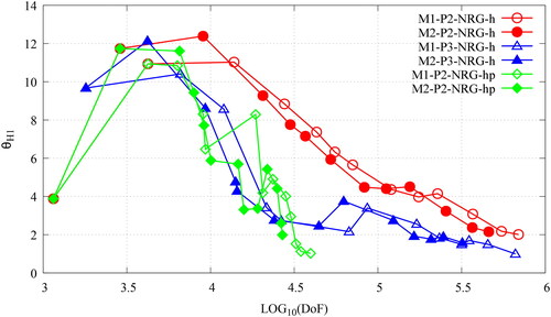
Figure 14. The spatial distributions of the multi-group components of the scalar neutron flux (left) and the scalar neutron importance (right) of the 2G NDE for the 2D IAEA/ANL BSS-11 benchmark. The QoI is the ${\mathrm{k}}_{\text{eff}}.$ (V. the web-based version for reference to color.).

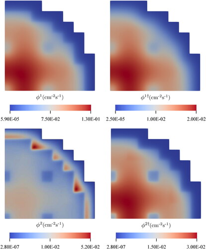
Figure 15. The energy-independent meshes (top) and the energy-dependent meshes (middle and bottom) generated at the $9^{\mathit{\text{th}}}$ AMR-iteration of the NRG-AMR-h (left) and the DWR-AMR-h (right) of the SIP-DG-IGA 2G NDE for the 2D IAEA/ANL BSS-11 benchmark. The QoI is the ${\mathrm{k}}_{\text{eff}}.$ (V. the web-based version for reference to color.).

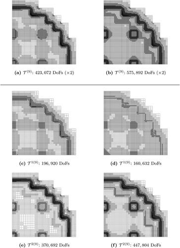
Figure 16. The energy-independent meshes (top) and the energy-dependent meshes (middle and bottom) generated at the $9^{\mathit{\text{th}}}$ AMR-iteration of the NRG-AMR-hp (left) and the DWR-AMR-hp (right) of the SIP-DG-IGA 2G NDE for the 2D IAEA/ANL BSS-11 benchmark. The QoI is the ${\mathrm{k}}_{\text{eff}}.$ (V. the web-based version for reference to color.).

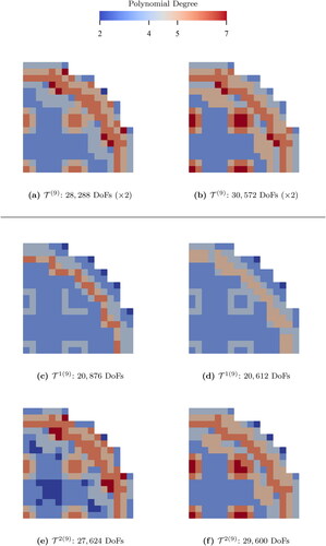
Figure 17. The convergence plots, ϵ_QoI v DoFs, for the uniform refinement (black), the NRG-AMR (red) and the DWR-AMR (blue) of the SIP-DG-IGA 2G NDE for the 2D IAEA/ANL BSS-11 benchmark. The prefixes M1- and M2- denote the use of energy-independent and energy-dependent meshes, respectively. The QoI is the ${\mathrm{k}}_{\text{eff}}.$ (V. the web-based version for reference to color.).

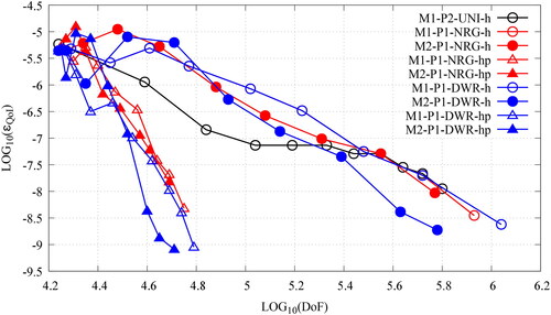
Figure 18. The spatial distributions of the multi-group components of the scalar neutron flux (left) and the scalar neutron importance (right) for the 2G NDE for the 2D BIBLIS benchmark. The QoI is the absorption in Material 5. (V. the web-based version for reference to color.).

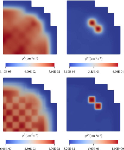
Figure 19. The energy-independent meshes (top) and the energy-dependent meshes (middle and bottom) generated at the $9^{\mathit{\text{th}}}$ AMR-iteration of the NRG-AMR-h (left) and the DWR-AMR-h (right) of the SIP-DG-IGA 2G NDE for the 2D BIBLIS benchmark. The QoI is the absorption in Material 5. (V. the web-based version for reference to color.).

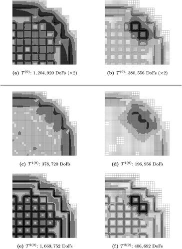
Figure 20. The energy-independent meshes (top) and the energy-dependent meshes (middle and bottom) generated at the $9^{\mathit{\text{th}}}$ AMR-iteration of the NRG-AMR-hp (left) and the DWR-AMR-hp (right) of the SIP-DG-IGA 2G NDE for the 2D BIBLIS benchmark. The QoI is the absorption in Material 5. (V. the web-based version for reference to color.).

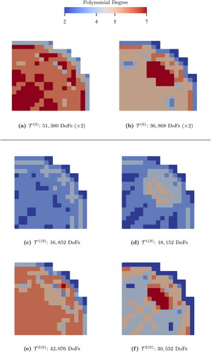
Table 5. The indicative timings for the different stages of analysis at the 9^th AMR-iteration of the NRG-AMR-h(p) and DWR-AMR-h(p) of the SIP-DG-IGA 2G NDE over energy-dependent meshes for the 2D BIBLIS benchmark.

Stage	NRG-AMR-h	NRG-AMR-hp	DWR-AMR-h	DWR-AMR-hp
Assembly	<1%	5%	1%	5%
Solution	6%	60%	11%	61%
Refinement	94%	35%	88%	34%
Total (s)	198	10	85	7

The Solution stage includes: evaluating the group-to-group sources over energy-dependent meshes. The Refinement stage includes: calculating the a posteriori interpolation-based error measures; and calculating the TICs for the optimized penalty parameters over the more-refined reference meshes.

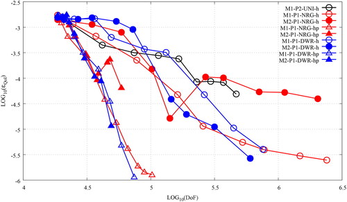
Figure 21. The convergence plots, ϵ_QoI v DoFs, for the uniform refinement (black) and the NRG-AMR (red) and the DWR-AMR (blue) of the SIP-DG-IGA 2G NDE for the 2D BIBLIS benchmark. The prefixes M1- and M2- denote the use of energy-independent and energy-dependent meshes, respectively. The QoI is the absorption in Material 5. (V. the web-based version for reference to color.).

Wilson, S. G., M. D. Eaton, and J. Kópházi. 2024. Energy-dependent, self-adaptive mesh h(p)-refinement of a constraint-based continuous Bubnov-Galerkin isogeometric analysis spatial discretization of the multi-group neutron diffusion equations with dual-weighted residual error measures. Journal of Computational and Theoretical Transport 53:1–64. 10.1080/23324309.2024.2313460.

 Web of Science ®Google Scholar

Data statement

In accordance with EPSRC funding requirements, all supporting data used to create figures in this paper may be accessed via the following URL: https://doi.org/10.5281/zenodo.10370345.