Quantum simulation in Fock-state lattices

Figures & data

Figure 1. The FSLs of d-mode JC model [33]. (a) The FSL with d = 2 is a 1D SSH lattice (N = 5). (b) The FSL with d = 3 is a 2D honeycomb lattice (N = 5). (c) The FSL with d = 4 is a 3D diamond lattice (N = 3). The two sublattices are denoted by the balls and squares, and the numbers $n_1{n}_2\dots n_d$ labelling the sites are the photon numbers in the d modes. The coupling strengths are proportional to the widths of lines connecting neighboring sites. Here we set the vacuum coupling strengths of all d modes equal, i.e. $g_j=\mathit{g}$.

Figure 2. The topological defect transfer in 1D FSLs. (a) The probability distribution of topological defect states (solid lines) localized at the topological edge (dashed lines). The vacuum coupling strengths are $g_1=g_0\text{sin}\mathit{\theta }$ and $g_2=g_0\text{cos}\mathit{\theta }$ [33]. (b) Transport fidelity as a function of the total transport duration T. The transfer can be accelerated in the non-adiabatic regime (marked by the empty circles) [40]. (c) Robustness of the topological transport with different noise strength $\mathit{\delta }$ [40]. (d) False-color circuit image of the experimental device [34]. The main elements of the circuit consist of the central qubit Q₀ (green line) and three resonators $R_1,R_2,R_3$ as twisting lines in cyan, red and yellow, respectively. The resonators and the qubit are coupled via couplers (two-circle elements in blue), which are used for tuning the coupling strengths. The purple lines indicate the ancilla qubit used for preparation and readout of the resonators. Inset: schematic of the main elements a central qubit Q₀ (green) coupled to three resonators R₁ (cyan), R₂ (red) and R₃ (yellow). (e) Experimental observation of the defect state transport for an initial state $|\downarrow ,0,5⟩$. The photons are transferred from R₂ to R₁ at around t = 600 ns [34].

Figure 3. The PMFs, pseudo-Landau levels and geometric phases. (a) The distribution of the strain-induced PMF, $\mathit{B}(\mathbf{r})/B_0^{+}$. The PMF is induced by the inhomogeneous hopping strengths inside the incircle of the lattice. The Dirac points are shifted as if being coupled to a vector potential [33]. (b) Experimental observation of the pseudo-Landau levels. The upper panel shows the evolution of the excited state population. Green dots and black line represent the experimental data and numerical simulation. The frequency components are shown in the bottom left panel by performing the fast Fourier transform of the Rabi oscillation, which agrees with the theoretically predicted $\sqrt{\mathit{n}}$-energy spectra in the bottom right panel [34]. (c) The equivalence between the Berry phase of the pseudo-spin and the AB phase induced by the PMF in lattice [47].

Figure 4. The valley Hall effect in 2D FSLs [34]. (a) The evolution of the wavefucntion distribution in the FSL. The directions of the trajectories are perpendicular to the effective electric fields (arrow) and opposite on two valleys, due to the opposite signs of the PMF. The size of the dots indicates the population of the states. (b) The evolution of the averaged photon numbers in resonators for the coherent initial state $|\downarrow ,\mathit{\alpha },0,-\mathit{\alpha }⟩$ ($\mathit{\alpha }\approx 1.8$). Photons are exchanged between resonators without exciting the qubit. (c) The measured Wigner functions of the three resonator states at time t = 100 and 290 ns, showing opposite chirality of the states in the two valleys.

Figure 5. The Haldane model in FSLs. (a) The spectrum of the FSL Haldane hamiltonian $H_{\text{H}}$. The color depicts the spin polarization $⟨{\sigma }_z⟩$. The edge modes connect the upper and lower bands [33]. (b) The evolution of the averaged photon number in resonators shows the chiral edge current, which is realized by periodically modulating the coupling strengths [34,48]. (c) The phase diagram of the generalized Haldane FSL with hamiltonian $H_{\text{H}}^{\prime }$. The color depicts the value of the topological marker near the lattice center [33].

Figure 6. Generating NOON states through the quantum transistor. (a) The state evolution in the FSL with the spin-orbit coupling hamiltonian. The inset shows sublattice-dependent phases of the NNN hoppings. The blue (red) dots represent the probability amplitude on the $\uparrow$ ($\downarrow$) sublattice. $\mathit{T}$ is the time to complete photon exchange between cavities [48]. (b) Schematic configuration of the quantum transistor. The cavity 1 is the input and cavity 2 and 3 are the outputs. The output state is controlled by the quantum state of the qubit [49]. (c) The quantum circuit scheme for preparing NOON states with N = 10. Each line represents an inseparable state. n_j is the photon number of the jth cavity. The block ${\theta }_j$ denotes the $\mathit{\theta }$ Rabi rotation between the jth cavity and the qubit. $H_{\text{so}}$denotes the state evolution under the effective Haldane term for time $\mathit{T}$ [48].

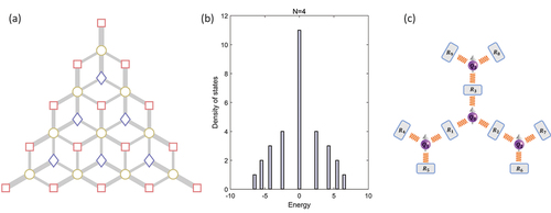
Figure 7. Extensions of the multi-mode JC model. (a) Fock-state lattice of JC models with three cavities being coupled to two atoms. The three types of sites correspond to $|\downarrow \downarrow ⟩$ (squares), $(|\downarrow \uparrow ⟩+|\downarrow \uparrow ⟩)/\sqrt{2}$ (circles) and $|\uparrow \uparrow ⟩$ (diamonds). The total excitation number N = 4. (b) The energy spectrum of the FSL in (a). Compared to the FSL with only one atom, the zero-energy level has a much higher degeneracy, containing a flat band due to the dice lattice configuration. (c) Schematic design of an atom-resonator lattice with a high dimensional FSL for unexplored topological states.

Cai H, Wang DW. Topological phases of quantized light. Nat Sci Rev. 2020 08;8:nwaa196. doi: 10.1093/nsr/nwaa196

 PubMed Web of Science ®Google Scholar

Yuan J, Xu C, Cai H, et al. Gap-protected transfer of topological defect states in photonic lattices. APL Photonics. 2021;6. doi: 10.1063/5.0037394

 Web of Science ®Google Scholar

Deng J, Dong H, Zhang C, et al. Observing the quantum topology of light. Science. 2022;378:966–971. doi:10.1126/science.ade6219

 PubMed Web of Science ®Google Scholar

Yuan J, Cai H, Wu C, et al. Unification of valley and anomalous hall effects in a strained lattice. Phys Rev B. 2021 Jul;104:035410. doi: 10.1103/PhysRevB.104.035410

 Web of Science ®Google Scholar

Wang D-W, Cai H, Liu R-B, et al. Mesoscopic superposition states generated by synthetic spin-orbit interaction in fock-state lattices. Phys Rev Lett. 2016 Jun;116. doi: 10.1103/PhysRevLett.116.220502

 Web of Science ®Google Scholar

Li H, Cai H, Xu J, et al. Quantum photonic transistor controlled by an atom in a floquet cavity-qed system. Opt Express. 2019 Mar;27:6946–6957.

 PubMed Web of Science ®Google Scholar