Limiting downstream dispersal of invasive carp egg surrogates using a laboratory-scale oblique bubble screen

Figures & data

Figure 1. (a) Sketch of the setup in the racetrack flume. Cross section of the diffuser system (A-A’ in Figure 1(a)). Aeration tubing is attached to a steel pipe and a ramp made of split polyvinyl chloride (PVC) pipe (all dimensions in mm). (b) Picture for the overall setup focusing on the area around the diffuser seen from the downstream end of the oblique bubble screen (OBS) (photo credit: V. Prasad, UIUC); notice the surfacing bubble screen, mounted acoustic doppler velocimeter (ADV), and high-speed camera used for surface particle image velocimetry (PIV; red rectangle).

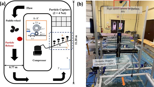
Figure 2. A schematic of the data acquisition using acoustic doppler velocimeter (ADV) while the diffuser is in operation. (a) ADV measurements with no crossflow (U₀ = 0). Each point denotes the location of measurement on the Central plane. (b) ADV measurements with mean flow. Each asterisk denotes the location of a vertical profile of eight points in the vertical. Surface particle image velocimetry (PIV) field of view shown in a green rectangle. The solid black line represents the diffuser, and the dotted grey line shows the approximate location of the bubbles when they approach the water surface [cm, centimetres].

Table 1. Summary of bulk flow parameters corresponding to the three nominal flow velocities (U₀), including near-bed turbulent kinetic energy (TKE_bed) and turbulence intensity percent (TI_bed × 100), Reynolds number (Re), Froude number (Fr), and shear velocity (u_*) [m, metres; cm, centimetres; s, seconds; Hz, Hertz].

No.	U0 (m/s)	Paddle frequency (Hz)	TKEbed (cm^2/s^2)	TIbed (%)	Re (×10^5)	Fr	Shear velocity at the bed (cm/s)
1	0.23	7	7.8	12.50	0.92	0.116	1.22
2	0.45	14	24.4	11.79	1.8	0.227	2.15
3	0.75	28	55.6	10.73	3.0	0.379	3.25

Table 2. Characteristics of the particles used as surrogates [mm, millimetres; cm/s, centimetres per second].

No.	Particle type	Mean diameter (mm)	Mean settling speed (cm/s)	Specific gravity	Shape, colour
1	Positively buoyant	7.10	Not applicable	0.9	Spherical, white
2	Negatively buoyant	5.90	7.2	1.04	Spherical, fluorescent green under UV light
3	Semi-buoyant	3.50	0.5	∼1.001	Hemispherical, white

Table 3. Physical properties of water-hardened invasive carp eggs determined by George et al. (2017).

No.	Species	Diameter (mm)	Terminal settling speed (cm/s)	Specific gravity
1	Grass carp (Ctenopharyngodon idella)	4.5 ± 0.6	0.74 ± 0.16	1.00068 ± 0.00052
2	Silver carp (Hypophthalmichthys molitrix)	4.7 ± 0.4	0.69 ± 0.07	1.00044 ± 0.00008
3	Bighead carp (Hypophthalmichthys nobilis)	5.8 ± 0.5	0.78 ± 0.07	1.00043 ± 0.00019

Note: Specific gravity was calculated for different temperatures using the data and methodology presented in George et al. (2017) [mm, millimetres; cm/s, centimetres per second].

Figure 3. (a) Schematic for proof-of-concept experiments using positively buoyant particles including the four general trajectories of particles based on their final location (A, B, C, D). (b) Photo of semi buoyant (SB) particles being redirected as they pass through the oblique bubble screen (OBS). (c) Picture of the eight-cell net used for particle capture. (d) Sketch showing dimensions of net cells. The blue dashed line in (c) and (d) denotes the water surface level. [θ, diffuser angle; B, channel width; cm, centimetres] (photo credits: V. Prasad, UIUC).

Table 4. Airflow rates for diffusers of different angles (θ) and lengths, where Q_a is the total airflow rate and q_a is the airflow rate per unit length of diffuser [m, metres; h, hours].

No.	θ (degrees)	Diffuser length (m)	Qa (m^3/h) for [high, low] airflows	qa (m^3/h/m) for [high, low] airflows
1	30	0.82	4.9, 1.5	6.0, 1.8
2	45	1.00	6.0, 1.8	6.0, 1.8
3	60	1.42	8.5, 2.6	6.0, 1.8

Figure 4. Mean velocity vectors generated by the bubble screen in the absence of crossflow with the diffuser aligned perpendicular to the flume (θ = 0°). the colour scales show mean velocity magnitude in centimetres per second (cm/s) in the x-z plane (u_xz).

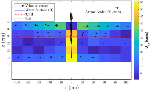
Figure 5. Mean velocities around the oblique bubble screen (OBS) in the y-z plane are shown using vectors. The colourmap shows streamwise mean velocity (U) as seen from the upstream (flow is into the page). The OBS system generated recirculation towards the downstream end of the diffuser [cm, centimetre].

Figure 6. Turbulent kinetic energy (TKE) calculated using acoustic doppler velocimeter (ADV) measurements for six cross-sections seen from upstream (flow is into the page). A zone of higher turbulence can be seen near the core of the bubble screen [cm, centimetre; s, second].

Figure 7. Mean velocity ratios |V|/|U| for three different mean flow velocities (U₀ = 0.23, 0.45, 0.75 metres per second [m/s]) at an airflow rate, q_a = 6 standard cubic metre per hour per metre length for the 60-degree diffuser [cm, centimetres].

Figure 8. Mean capture percentages for positively buoyant (PB) particles for different diffuser angles, mean flow velocities, and airflow rates (q_a, in cubic metres per hour per metre of diffuser [m³/h/m]): zero air flow (a), low air flow (b–d) and high air flow rates (e–g). A schematic of the net on top-left shows location of the cells with the flow going into the page. Error bars show the standard deviation in the three replicates for each configuration. Only one case was tried for the trial with zero airflow rate because all the particles stayed on the surface for all three angles of the diffusers [m/s, metres per second].

Figure 9. Capture percentages for negatively buoyant (NB) particles for different diffuser angles, mean flow velocities, and airflow rates (q_a, in cubic metres per hour per metre of diffuser [m³/h/m]): zero air flow (a–c), low air flow (d–f) and high air flow rates (g–i). Error bars show the standard deviation in the three replicates for each configuration [m/s, metres per second].

Figure 10. Mean capture percentages for semi-buoyant (SB) particles for different diffuser angles, mean flow velocities, and airflow rates (q_a, in cubic metres per hour per metre of diffuser [m³/h/m]): zero air flow (a), low air flow (b–d) and high air flow rates (e–g). Error bars are the standard deviation in the three replicates for each configuration [m/s, metres per second].

Figure 11. Effective redirection as a function of diffuser angle, mean flow velocity, and airflow rate for all three types of particles for all the configurations of the oblique bubble screen (OBS). (a), (b) and (c) show the plots for positively buoyant (PB), negatively buoyant (NB), and semi buoyant (SB) particles, respectively. Effective redirection is defined as the average percentage of particles captured in the rightmost column of the net (A4 and B4 in Figure 3) [deg, degrees; m/s, metres per second].

Figure 12. Correlation between the bulk velocity ratio (<|V|/|U|>; bars) and effective redirection for positively buoyant (PB) and semi buoyant (SB) particles (markers and trendlines) at high airflow rate. Error bars show standard deviation in three replicates for the selected configurations [deg, degrees; m/s, metres per second].

George AE, Garcia T, Chapman DC. 2017. Comparison of size, terminal fall velocity, and density of bighead carp, silver carp, and grass carp eggs for use in drift modeling. Trans Am Fish Soc. 146(5):834–843. doi: 10.1080/00028487.2017.1310136.

 Web of Science ®Google Scholar

Data availability statement

The authors confirm that the data supporting the findings of this study are available within the article and its Supplementary Material.