Feature extraction and spatial imaging of synchrotron radiation X-ray diffraction patterns using unsupervised machine learning

Figures & data

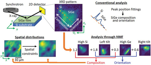
Figure 1. Schematic illustrations of the optical system of micro-beam XRD. (a) The incident X-ray beam was focused on the sample surface and the XRD pattern from the (022) plane was captured by a two-dimensional detector. Before the spatial mapping, the optical axes, α, ω, θ, and η, were adjusted to the (022) diffraction condition. (b) The effective spot size was estimated to be 13 μm in major diameter taking incident angle and diffraction from sample inside into account.

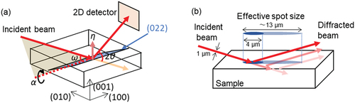
Figure 2. (a) Average pattern around (220) SiGe diffraction spots of 961 XRD patterns obtained in the spatial mapping. The pixel resolution and intensity were converted to 1/4 and the natural logarithm scale from the original two-dimensional detector image. The white dot shows the position corresponding to the (220) diffraction spot of fully relaxed Ge. (b) Positions of (220) diffraction spots of pure Si and Ge in the reciprocal space.

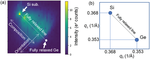
Figure 3. (a–d) typical XRD patterns obtained in the spatial mapping. The measured positions of (a–d) in the mapping area on the sample surface are (60, 150), (100, 135), (35, 65), (120, 55) in (x, y) in μm. The pixel resolution and intensity were converted to 1/4 and the natural logarithm scale from the original pattern measured by the two-dimensional detector. (e–h) XRD patterns reconstructed for the pattern (a–d) using the four feature patterns and their coefficents obtained through NMF. The reconstructed patterns using the other numbers (1–5) of feature patterns are provided in S5 in the supplemental information.

Figure 4. Feature patterns obtained by NMF with (a) one, (b) two, (c) three, (d) four, (e) five, and (f) six components. The order of the patterns was sorted to be similar patterns are arranged vertically for easy comparison. Dead pixels in the patterns are caused by the dead pixels of the detector. The feature patterns with 1–10 components are provided in S4 in the supplemental information. (g) Corresponding reciprocal space coordinate of the feature pattern images. The position in the direction along the fully relaxed line between the Si substrate and pure Ge represents the SiGe composition. In terms of crystal orientation, the position on the fully relaxed line corresponds to the crystal orientation alined to the Si substrate, and the area below and above the line represents the crystal orientation of left and right tilted around the incident X-ray beam, respectively. (h) Reconstruction error, which is evaluated by the Frobenius norm of the matrix difference in Equation (1) divided by the number of the diffraction patterns, for the 961 diffraction patterns of the models with one to six components. Reconstruction error with 1–10 components is also provided in S4 in the supplemental information.

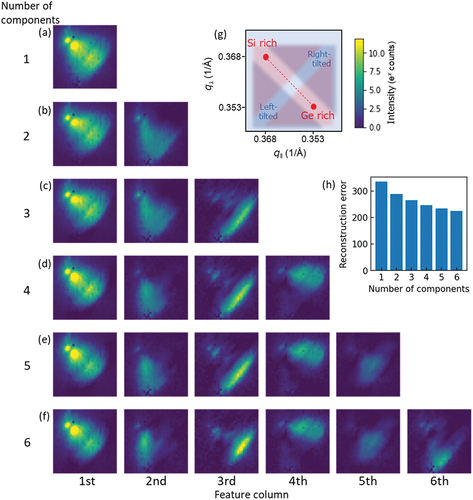
Table 1. Composition and tilt angle of crystal orientation calculated from the maximum spot position of the feature patterns of FIG. 4 (d). Positive tilt angle corresponds to left tilt.

Pattern No.	1	2	3	4
Composition	Si1.00Ge0.00	Si0.52Ge0.48	Si0.00Ge1.00	Si0.61Ge0.39
Tilt angle	0º	0.064º	0º	−0.087º

Figure 5. Spatial mapping images of the coefficients: (a) (coef. 4) – (coef. 2) and (b) (coef. 3) – (coef. 1) of the four feature pattens, and (c) coef. 6 of the six feature pattens. The orientation of both images along the direction from bottom left to top right is caused by the shape of the footprint of the X-ray beam.

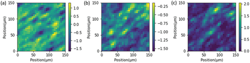
Figure 6. Feature patterns S_j obtained throuth NMF with spatial contraints, β = 0, 300, 1000 for (a), (b), (c). The virtical and horizontal direction correspond to q_⊥ and q_‖ in the reciprocal space, as in the case of FIG. 4. The order of the patterns was sorted to be similar patterns are arranged vertically for easy comparison. The subscript number j of S corresponds to the feature number common to those in FIG.7. The feature patterns obtained with other β values are provided in S7 in the supplemental information.

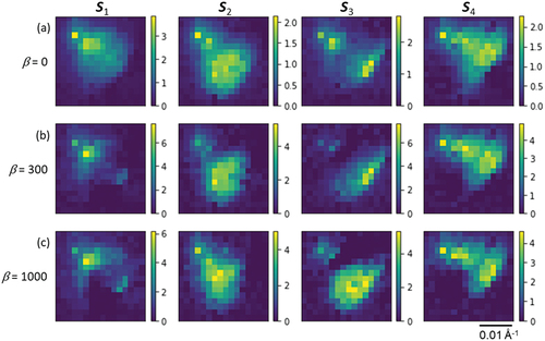
Figure 7. Spatial distribution of the coefficients C_j of the four features with spatial contraints, β = 0, 300, 1000. The subscript number j of C corresponds to the feature number in FIG.6. The spatial size of the images is 75 μm × 75 μm. The feature patterns obtained with other β values are provided in S8 in the supplemental information.

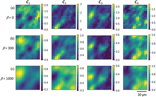
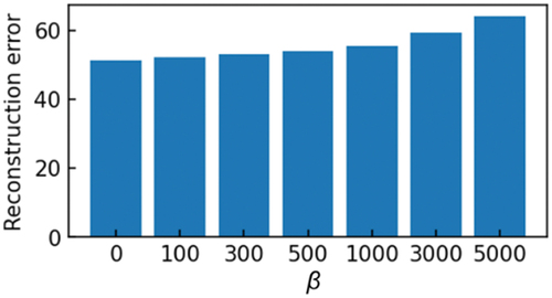
Figure 8. Reconstruction error of the models learned with different β. The error was evaluated by Frobenius norm of the matrix difference in Equation (2) divided by the number of the diffraction patterns.

Data availability statement

The data and the code that support the findings of this study can be found at https://github.com/KentaroKutsukake/NMF-for-XRD.git.