A hybrid brain-computer interface using motor imagery and SSVEP Based on convolutional neural network

Figures & data

Figure 1. Three modes of BCI system. (left top) MI mode, in which the subject imagines the left- or right-hand movement. (left bottom) SSVEP mode, in which the subject stares at the left or right flickering stimulus. (right) Hybrid mode, in which the MI and SSVEP are combined.

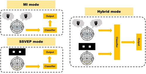
Figure 2. The TSCNN framework: (A) EEG Recording and preprocessing: the recorded EEG is filtered by $8\sim 30Hz$ bandpass filter, and then segmented into 4s length. (B) Channel selection: select the specific channels of MI and SSVEP. (C) Classification: classify the input EEG segments with TSCNN.

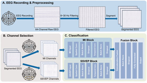
Table 1. Decoding performance (mean ± std) of three models.

Model	Paradigm	Accuracy	Sensitivity	Specificity	MSE
SCNN	MI	0.704 ± 0.008	0.703 ± 0.020	0.706 ± 0.023	0.575 ± 0.003
	SSVEP	0.937 ± 0.003	0.931 ± 0.010	0.944 ± 0.009	0.119 ± 0.00
	MI	0.678 ± 0.017	0.764 ± 0.078	0.591 ± 0.099	0.609 ± 0.019
TSCNN1	SSVEP	0.934 ± 0.004	0.937 ± 0.018	0.931 ± 0.01	0.126 ± 0.004
	Hybrid	0.956 ± 0.006	0.961 ± 0.011	0.952 ± 0.018	0.100 ± 0.005
	MI	0.702 ± 0.007	0.709 ± 0.028	0.695 ± 0.024	0.583 ± 0.006
TSCNN2	SSVEP	0.930 ± 0.006	0.943 ± 0.013	0.916 ± 0.020	0.134 ± 0.005
	Hybrid	0.956 ± 0.006	0.964 ± 0.007	0.948 ± 0.013	0.110 ± 0.004

The table highlights the maximum value in bold.

Table 2. Comparison of mean ± standard deviation for decoding performances (mean ± std) in single MI, SSVEP, and hybrid systems.

Mode	Model	Accuracy	Sensitivity	Specificity	MSE
MI	SCNN	0.704 ± 0.008	0.703 ± 0.020	0.706 ± 0.023	0.575 ± 0.003
	1DMSCNN [34]	0.693 ± 0.047	0.711 ± 0.055	0.683 ± 0.065	0.307 ± 0.047
	SCNN	0.937 ± 0.003	0.931 ± 0.010	0.944 ± 0.009	0.119 ± 0.00
SSVEP	MFCNN [9]	0.929 ± 0.035	0.945 ± 0.031	0.919 ± 0.059	0.710 ± 0.35
	CFCNN [9]	0.941 ± 0.012	0.951 ± 0.026	0.933 ± 0.031	0.59 ± 0.12
	hSCNN	0.786 ± 0.179	0.787 ± 0.165	0.85 ± 0.018	0.214 ± 0.179
Hybrid	TSCNN1	0.956 ± 0.006	0.961 ± 0.011	0.952 ± 0.018	0.100 ± 0.005
	TSCNN2	0.956 ± 0.006	0.964 ± 0.007	0.948 ± 0.013	0.110 ± 0.004

The table highlights the maximum value in bold.

Table 3. Decoding accuracy of TSCNN2 according to the fully connected number.

Mode	MI	SSVEP	Hybrid
without fully-connected layer	0.651	0.936	0.956
16-dimension fully-connected layer	0.704	0.937	0.956

The table highlights the maximum value in bold.

Table 4. Decoding accuracy of TSCNN2 according to the number of convolution kernels.

Convolution kernels	(1, 1)	(1, 2)	(2, 2)	(8, 8)
MI	0.704	0.663	0.662	0.646
SSVEP	0.937	0.935	0.933	0.930
Hybrid	0.956	0.957	0.954	0.947

The table highlights the maximum value in bold.

Figure 3. Impact of TSCNN architecture design choices on decoding accuracy in MI mode (left), SSVEP mode (middle), and hybrid mode (right) with different dropout rates. The horizontal axis is the different dropout rates, and the vertical axis is the decoding accuracy.

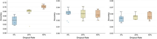
Figure 4. Impact of TSCNN architecture design choices on decoding accuracy in MI mode (left), SSVEP mode (middle), and hybrid mode (right) with different activations. The horizontal axis is the different dropout rates, and the vertical axis is the decoding accuracy.

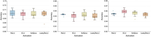
Figure 5. Visualization of features for subjects 20–30 in 2 dimensions using t-SNE– – TSCNN2. (a)–(c) are the visualization results in MI block. (a) MI input features. (b) Features of spatial convolutional layer in MI block. (c) Features of the temporal convolutional layer in MI block. (d)-(e) are the visualization results in SSVEP block. (d) SSVEP input features. (e) Features of the spatial convolutional layer in SSVEP block. (f) Features of the temporal convolutional layer in SSVEP block. (g) Is the visualization result of fully-connected layer.

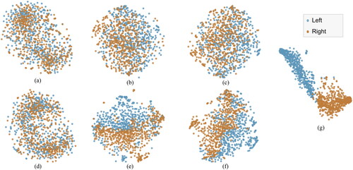
Figure 6. The ratio according to different thresholds. The thresholds are the weights of connections that are relatively high. The vertical axis is the ratio of the number of connections exceeding the threshold in TSCNN1 to the number in TSCNN2. The blue curve is the ratio in TSCNN1, and the red curve is the ratio in TSCNN2.

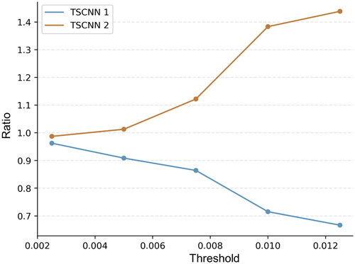
Table 5. The number of weights that are greater than the threshold.

Model	Threshold	0.0025	0.005	0.0075	0.01	0.0125
	NM	29713	9699	2374	407	64
TSCNN1	NS	30870	10674	2747	569	96
	Ratio	0.963	0.909	0.864	0.715	0.667
	NM	30121	10219	2665	534	82
TSCNN2	NS	30510	10089	2375	386	57
	Ratio	0.987	1.013	1.122	1.383	1.439