Statistical modelling under differential privacy constraints: a case study in fine-scale geographical analysis with Australian Bureau of Statistics TableBuilder data

ABSTRACT

Consistent with the principles of differential privacy protection, the Australian Bureau of Statistics artificially perturbs all count data from the Australian Census prior to its release to researchers through the TableBuilder platform. This perturbation involves the addition of random noise to every non-zero cell count followed by the suppression of small values to zero. A consequent problem encountered by researchers working with geographical TableBuilder outputs is that the aggregate sums of cell counts over fine-scale units are often much lower than the direct query totals of their coarser enclosing units. Hierarchical Bayesian modelling is here proposed as a powerful methodology for achieving consistent multi-scale statistical reconstructions suitable for downstream spatial modelling. The utility of this framework is demonstrated for the toy problem of reconstructing Multiple Family Household counts by Mesh Block in the Perth Greater Capital City area.

KEYWORDS:

• Census population counts
• TableBuilder
• Australian Bureau of Statistics
• data perturbation
• differential privacy
• Bayesian statistics

Introduction

Data summaries from the Australian Census are made available by the Australia Bureau of Statistics (ABS) to researchers at approved institutions through the TableBuilder platform.¹ Users with permission to run queries at the TableBuilder Pro tier can request counts of dwellings, households or persons stratified along selected Census attributes in up to three dimensions (rows, columns and ‘wafers’; the later being the ABS terminology for the third data dimension in an array). Example attributes are the place of usual residence, age, sex, household size or country of birth. Spatial stratifications may be specified according to the nested Australian Statistical Geography Standard (ASGS)², the finest three levels of which are Mesh Blocks (containing around 30–60 dwellings in most instances), SA1 units (around 200–800 people) and SA2 units (3,000–25,000 people). TableBuilder outputs are widely used in spatial epidemiology and geographical research. Examples include the mapping of gay and lesbian population clusters (‘gayborhoods’) by postcode (Callander et al. 2020), the study of associations between socio-economic indices and migrant population densities at ‘suburb’ (SA2) level (Colic-Peisker and Peisker 2022) and the construction of virtual populations at SA1 level for computational influenza modelling (Zachreson et al. 2018).

To preserve the confidentially of individual records in the Australian Census, the ABS have developed a methodology for perturbing the true counts by Census attribute, such that those returned by TableBuilder are in fact noisy, censored versions of the originals (Chipperfield, Gow, and Loong 2016). Although the early development of this algorithm was not shaped explicitly by differential privacy theory, it has subsequently been analysed through this lens and found to be broadly consistent with its principles and aims (Bailie and Chien 2019; Rinott et al. 2018). Namely, to effectively share information about groups of individuals without exposing the individual data to more than a tiny risk of probabilistic de-identification. Rinott et al. (2018) note:

‘It is a property of differential privacy that the confidentiality protection guarantee does not rely on hiding the parameters of the perturbation. … [hence] knowledge of the mechanism allows the user to take the perturbation distribution into account in their analysis for data independent algorithms’

A number of publications from the ABS give insight into the nature of the perturbation methodology applied within TableBuilder, although in fact none of these documents provide sufficient information from which to precisely reconstruct the noise generation process (Chipperfield, Gow, and Loong 2016; Giessing 2016).

Two recent studies have presented algorithmic methodologies to facilitate geospatial analyses of sparse TableBuilder outputs at fine spatial scales. In Australian Geographer, Kok et al. (2022) consider the challenge of mapping incidence rates of high-risk foot hospitalisations amongst the Indigenous population of Perth. They demonstrate that the suppression of population counts for Indigenous residents filtered by age group at the SA1 scale creates two problems for the analyst. First, some SA1 areas with attributed hospital address records have zero population output from TableBuilder, yielding an improper zero denominator for the crude incidence rate. Second, the aggregations of SA1 TableBuilder population totals within their enclosing SA2 boundaries are in many cases markedly below the equivalent TableBuilder outputs returned on querying the SA2 population totals directly. With these issues in mind the authors propose a ‘map overlay technique’ in which many separate incidence ‘hotspot’ maps are created from the one set of TableBuilder outputs viewed across randomised aggregations of the SA1 units, from which a fine-scale product is subsequently synthesised using AZTool.

In Nature Scientific Data, Fair, Zachreson, and Prokopenko (2019) consider the problem of reconstructing the commuter networks of Greater Sydney using TableBuilder outputs of journey counts from place of residence to place of work (POW). The finest scale used for the former is SA1 and for the latter is the destination zone (DZN). The authors demonstrate the systematic impacts of low count suppression on the network structures built using the outputs available at these and coarser spatial scales. They further propose an algorithm for simulating a reconstructed network of SA1 to POW-DZN connections that matches approximately the SA2 to POW-DZN totals. Random out-edges from each SA1 are proposed from a normalised distribution of edge weights given the residential population of that SA1. Candidate in-edges to POW-DZN are then proposed considering SA2 to POW-DZN totals, SA2 to POW-SA2 totals and the associated POW-DZN incoming total from TableBuilder. It is noted that no new SA2 to POW-SA2 connections will be added by this method.

Absent from both the algorithms mentioned above is an explicit model for the perturbation process. By writing down a mathematical description of the process of random noise addition and low count suppression the analyst may gain access to the power of likelihood-based statistical modelling. In both the classical (‘Frequentist’) and Bayesian frameworks a great many theorems and techniques for estimating parameters, quantifying uncertainties and testing model suitability begin from this starting point (Held and Bové 2020). In the present problem setting the (multivariate) parameter we aim to estimate is the matrix of true cell counts at the finest geographical unit system under consideration; that is, the Mesh Block cell counts that were compiled by the ABS from the Census itself, before the perturbation and low count suppression steps were applied in TableBuilder. The true cell count within any coarser unit system of the nested ASGS hierarchy must be strictly equal to the sum over the true cell counts of all enclosed Mesh Blocks. Adding this constraint to the likelihood formulation enforces a benchmarking across the nested units during parameter inference.

In this manuscript we illustrate a Bayesian approach to likelihood-based inference on geographical TableBuilder outputs through a case study. Our case study concerns the toy problem of mapping the distribution of Multiple Family Households at the Mesh Block level within central Perth. We refer to this a ‘toy problem’ because the variable of interest was intentionally chosen for its relatively impersonal character (compared with Indigeniety or health status, for example), as well as its rareity which serves to illustrate the impact of zero suppression. Nevertheless, it is worth noting that multiple family homes are considered undesirable within the prevailing mainstream narrative (Munzner and Day 2015), so even this attribute carries a cost if individual re-identification is achieved. We must therefore emphasise that individual record re-identification is not an objective or outcome of this work.

As this is a Bayesian analysis, we will propose a suitable prior to complement the likelihood function. For our case study we have chosen a geospatial prior that combines regression on Mesh Block land use category and SA1 socio-economic status with spatial smoothing. A Markov Chain Monte Carlo procedure is then created for sampling from the Bayesian posterior of the resulting model. The outputs of this model are statistical reconstructions of plausible Mesh Block level counts of Multiple Family Households that are consistent with the multi-scale geographical TableBuilder outputs as interpreted through the likelihood function and prior. The nature of these model-based reconstructions and the performance of their associated uncertainty measures are examined using established techniques for model checking and evaluation.

Methods

Minimal perturbation model

High level details of the perturbation procedure applied to ABS TableBuilder outputs available on the ABS website are as follows:

• ‘As perturbation is applied independent of the size of a count, any individual count or total in Census data products will be no more than a very small number away from the unperturbed value.’³

• ‘Perturbation includes the suppression of small counts so individual information cannot be determined. This is why you’ll never see counts of 1 or 2 in Census output.’⁴

• ‘Perturbation is applied across all non-zero cells in a table, including the totals cells.’⁵

A simple statistical model of this process is to suppose that for each cell with a true cell count greater than zero the perturbation algorithm draws a replacement value at random from a discretised Normal distribution centred on the true cell count (that is, from a bell-shaped distribution constrained to only return integer values). Any cells with replacement values 2 or less are then set to zero. A formal mathematical description of this model is given in the Appendix for reference. Treating the true cell counts here as unknown parameters and fixing the perturbed values to their TableBuilder outputs turns this perturbation model into a likelihood-function ready for statistical inference (Held and Bové 2020).

Published descriptions of the perturbation modelling techniques developed by the ABS, however, indicate that the actual perturbation algorithm is much more complicated than the minimal version proposed above. Crucially, the error perturbations are not drawn independently for every cell in every possible query, but are pre-compiled from a pseudo-random number table generated against the individual micro-census records of persons, families and households (Marley and Leaver 2011; Thompson, Broadfoot, and Elazar 2013). The scale of the applied perturbations may also be varied on a per-query or per-record basis according to the sensitivity of information at-risk of disclosure (Marley and Leaver 2011). An alternative perturbation algorithm that mimics this behaviour is described in the Appendix. However, the complexity of this algorithm is such that its transformation into a likelihood function is not computationally feasible.

Inference under misspecification

The framework under which inference with the minimal perturbation model proposed here will thus be considered is that of Bayesian modelling under misspecification (Gelman and Shalizi 2013). That is, we will acknowledge from the beginning that our likelihood function does not truly represent the perturbation process applied in TableBuilder and we will turn our attention to assessing whether or not it may nevertheless be adequate for our purpose. To this end we use mock data simulations created under both the minimal and alternative perturbation models to test the performance of our statistical reconstruction procedure in both the well-specified and misspecified settings, respectively. If any degradation of performance under the misspecified setting relative to the well-specified one is acceptably small then we will conclude that the minimal perturbation model provides a satisfactory proxy for analysing real TableBuilder outputs.

Scale of injected noise

If one compares the output row totals against row sums for combinations of TableBuilder categories and areal units in which all entries are far from zero (e.g. counts of residents by sex at SA2 level), the empirical standard deviation of their difference is always close to $2\times \sqrt{M+1}$ where $M$ is the number of attributes. Supposing each random variate contributes equally to the standard deviation the root sum of squares rule suggests an error scale of 2 counts. If we assume that each sufficiently large population cell contains a number of individuals with high sensitivity scores we must conclude that 2 is an upper bound to the TableBuilder perturbation scale. We treat it explicitly as such in our alternative perturbation model which is defined so that many cells receive noise contributions of smaller scale. For simplicity in our minimal perturbation model we conservatively apply a noise scale of 2 counts across all geographical strata, acknowledging again that this model is misspecified relative to the true perturbation process.

Tablebuilder dataset

The primary dataset for our case study consists of TableBuilder outputs of counts for the Perth Greater Capital City (GCC) region stratified by place of residence and the 1-digit level Family Household Composition (HCFMD) attribute. There are 27,112 Mesh Blocks, 4,822 SA1 units and 185 SA2 units covering the Perth GCC and the HCFMD attribute has four categories: ‘Multiple Family Household’, ‘One Family Household’, ‘Other Household’ and ‘Not Applicable’. We statistically reconstruct all categories in our analysis, but focus our attention on the Multiple Family Household count. The sum totals of Multiple Family Households across the Perth GCC returned by TableBuilder at each spatial scale are 7,000 at Mesh Block level, 11,870 at SA1 level and 12,653 at SA2 level. This illustrates the under-estimation effect of the perturbation process at fine spatial scales noted by Kok et al. (2022).

Geospatial priors

In geographical statistical analyses it is common to introduce hierarchical priors that combine information from spatially varying covariates with the expectation of residual auto-correlation across nearby spatial units (Bhatt et al. 2015; Held et al. 2019). We propose that priors of this form can also be readily and effectively used to tune TableBuilder count reconstructions to the purpose of a given scientific analysis. For our case study we divide the problem of estimating the Multiple Family Household count at the Mesh Block level into two parts: first we estimate the total dwelling count in that Mesh Block and then we estimate the proportion of those dwellings that are Multiple Family Households.

To this end we introduce the Mesh Block land use category (available in the ASGS Mesh Block shapefile) and the SA1 areal Index of Relative Socio-Economic Advantage and Disadvantage decile (IRSAD; available from TableBuilder) as categorical regression covariates. All Mesh Blocks are assigned to one of ten categories (including ‘Residential’, ‘Commercial’ and ‘Industrial’) on the basis of the majority land use within their domain. The IRSAD is an areal estimate of socio-economic status produced by the ABS from the first principal component score over 23 Census variables; these include the proportion of residents aged over 15 years old with no higher education and the proportion of individuals living in households with stated annual household income over $91,000 AUD. The choice of these covariates for use in this toy problem was determined largely by their ready availability as well as their expected connection to dwelling type (e.g. more apartments in majority commercial areas) and probability of over-crowding (higher in low-income areas). Other suitable covariates that might be explored in a deeper analysis could include geospatial data summaries of building footprints and heights and/or additional demographic and socio-economic indicators. Similarly, alternative regression formulations using the precise IRSAD scores (rather than the deciles used here) for each area⁶ could be explored.

To the above two regression terms we add a spatial random effect defined as a Gaussian random field with Matérn covariance function and nugget, implemented computationally via a mesh-based approximation with INLA (Bakka et al. 2018) and TMB (Osgood-Zimmerman and Wakefield 2022). A full mathematical description of this model is given in the Appendix and the corresponding codes are made publicly available in the Online Repository.

Markov Chain Monte Carlo algorithm

The posterior of the above Bayesian model is intractable to closed form analytic evaluation, meaning that it is necessary to seek a computational posterior approximation. While many posterior approximation problems may be readily solved through an ‘off-the-shelf’ sampling codes (such as Stan or JAGS), statistical reconstruction of count data poses two particular challenges for efficient representation in standard probabilistic programming languages. First, the handling of structural zeros (i.e. true zero cell counts) and the production of random zeros through noise addition and suppression requires rule-based case handling. Second, the parameter space is discrete (i.e. non-negative integer valued counts), which rules out gradient-based sampling methods (such as hybrid Monte Carlo) designed for continuous random variables. Given these challenges we instead develop our own Markov Chain Monte Carlo procedure. This procedure takes the form of a blocked Gibbs sampler (Roberts and Sahu 1997), whereby the geospatial prior is updated as a regression model against the current setting of the Mesh Block counts and the counts are then updated against the current setting of the geospatial prior. The numerical implementation of this posterior sampler in R is again made publicly available in the Online Repository.

Model performance metrics

An established approach to investigate the behaviour of Bayesian models is to compare their posterior distributions against a ground truth (Gelman and Shalizi 2013). Since the ground truth for the real Census dataset is unknown to us we instead use mock datasets for this purpose. Specifically, we choose a posterior sample from our model fitting against the real TableBuilder outputs as our (artificial) ground truth, and then re-fit our model to mock datasets generated from this by applying either our minimal or alternative perturbation model. Two useful metrics of model performance can be computed in this way. The first of these is the Bayesian ‘coverage’, which examines the proportion of ground truth count values that are contained within the posterior 95% credible intervals at each areal level. While Bayesian credible intervals are not guaranteed to deliver Frequentist style performance, meaning that they would enclose at least the nominal fraction of true values, pathological under-coverage is frequently a consequence of model misspecification (Müller 2013). The second metric we compute is the area under the receiver operating curve (AUC) when using the posterior mean cell count of Multiple Family Households as a classifier of whether or not there is at least one dwelling of that type in the corresponding Mesh Block. This metric probes the in-fill accuracy of the model at its finest spatial scale.

Results

Multi-scale Bayesian reconstructions

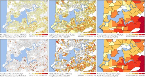
In Figure 1 we present a series of maps for a section of central Perth showing the posterior mean estimates of the number of Multiple Family Household dwellings per Mesh Block, SA1 and SA2 unit, as reconstructed with our geostatistical model. The TableBuilder outputs that served as inputs to this model are shown below the reconstruction at each areal scale for reference. The impact of low count suppression on the TableBuilder outputs at fine areal scales is readily observed in the sparsity of these maps at Mesh Block and SA1 levels, as is the impact of the model in attempting to probabilistically redistribute the counts known to be missing from consideration of the SA2 totals. Another effect of the model that is also readily apparent is the smoothing of high values from the TableBuilder outputs: under the assumed perturbation model, a cell count that survives the thresholding step is more likely to have been boosted by a positive random perturbation than reduced by a negative one.

Figure 1. Model-based reconstructions of the spatial pattern across central Perth of dwellings classified as containing Multiple Family Households (top row) compared against the perturbed input data from TableBuilder (bottom row). The colour scales for each areal unit (from Mesh Block on the left to SA1 in the middle and SA2 on the right) have each been tailored to highlight the underlying patterns.

Importantly, since this is a fully statistical reconstruction approach, both samples from the posterior and posterior uncertainty summaries are also readily produced. In Figure 2 we present two posterior samples as plausible maps of the Multiple Family Household dwelling count at Mesh Block level. Each posterior sample represents one of many possible worlds consistent with the available data as interpreted through the likelihood function and prior. In some areas the presence of at least one Multiple Family Household in the enclosing SA1 unit is indicated by the data, but the model remains uncertain as to which Mesh Block it belongs; while in other areas the model is confident from the available data that one or more specific Mesh Blocks are host to Multiple Family Household dwellings. Importantly, in each of these possible worlds the sums of dwelling type counts across areal units will be both internally consistent within the hierarchy and faithful to the input data.

Figure 2. Two posterior samples of the Multiple Family Household count by Mesh Block for central Perth (left & middle), and the width of the 95% posterior credible interval over all posterior samples (right).

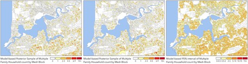
We also show for reference in Figure 2 the width of the ‘pointwise’ posterior 95% credible interval at Mesh Block level. Here we see that the typical 95% credible interval on a Mesh Block is in the 2–5 counts range or less, which reflects foremost the scale of the random noise in the error model. Across all posterior samples the land use categories and IRSAD deciles used as covariates in our geostatistical model explain an average of 84% of the spatial variance in the total dwelling count and 93% of the variance in the proportion of Multiple Family Households; hence in this example the spatial random field plays only a minor role in the model fitting. For the variance decompositions and modelled uncertainty intervals shown above to have real value, however, we must also establish confidence that the model is likely to be well-performing despite the known misspecification in our chosen likelihood function. Addressing this challenge is the focus of the remainder of the Results presented here.

Assessments of model performance

By performing statistical reconstructions on mock datasets generated under the minimal perturbation model we estimate mean global coverage fractions for our 95% credible intervals of 0.98 at Mesh Block level, 0.97 at SA1 level and 0.96 at SA2 level. Since in this case the perturbation applied is the same as that assumed by the likelihood function we are operating in the well-specified setting. The adequacy of these coverages against the specified value of 0.95 therefore confirms only that our Markov Chain Monte Carlo sampler is performing correctly and that the model does not suffer any unusual pathologies. More interesting is the misspecified setting, which is investigated by performing statistical reconstructions on mock datasets generated under the alternative perturbation model. In this case, we find mean global coverage fractions of 0.97 at Mesh Block level, 0.97 at SA1 level and 0.99 at SA2 level. A decline in coverage is an often-encountered problem for Bayesian inference under misspecification, yet here all coverages remain above the specified level.

A similar picture emerges in comparison of the AUC for the receiver operating characteristic which is 0.89 in the well-specified setting and 0.84 in the misspecified one. An AUC score of around 0.8–0.9 is generally considered favourable, although this is ultimately a subjective judgement to be made relative to the purpose of the analysis (de Hond, Steyerberg, and van Calster 2022). More importantly here is that the degradation of AUC performance introduced by misspecification in this case is small relative to the well-specified benchmark. As such, if our individual record perturbation model is indeed a faithful representation of the true perturbation model applied in TableBuilder we may conclude that the consequences from its approximation by our minimal perturbation model in the likelihood function are minor.

Discussion

In their Australian Geographer paper identifying the challenges of working with ABS TableBuilder outputs, Kok et al. (2022) highlight the importance of disease maps for the estimation of disease burden and resources allocation by reference to the work of the Malaria Atlas Project (Hay et al. 2005; Hay et al. 2013). In 2020 MAP relocated from the University of Oxford to the Telethon Kids Institute in Perth, Western Australia, adding to the strengths of the Australian infectious disease mapping community. A guiding principle of MAP’s work has always been that when working with disease data a statistical approach is essential to ensure that the uncertainties attached to disease maps can be communicated clearly to the intended audience of policy makers, researchers and the general public. Importantly, Hay and Snow (2006) note that:

‘A very considerable research effort is also required to evaluate those statistical techniques needed to relate the PR [prevalence] and environmental data for extensive map predictions with confidence intervals.’

That is, the challenge for researchers working in this field is not only to develop novel statistical methods for disease mapping, but also to subject those methods to scrutiny to ensure that their performance can be monitored and improved over time.

In this study, we have demonstrated that a likelihood-based statistical treatment of the ABS TableBuilder outputs is both feasible and effective using a Bayesian methodology. Specifically, we have demonstrated that under a simple approximation for the incompletely known perturbation procedure, posterior sampling under a geospatial regression prior can be achieved through Markov Chain Monte Carlo. Moreover, we have interrogated the performance of this model in both the well-specified regime (i.e. with mock datasets simulated under the assumed perturbation model) and in the misspecified regime (i.e. with mock datasets simulated under an alternative perturbation model thought to be closer to the true TableBuilder perturbation process). We have made all code for reproducing these experiments available to other researchers in an Online Repository. Further work is warranted in a number of possible research directions to build on this foundation.

While we have focussed on likelihood-based inference in this case study, it is worth noting that ‘likelihood-free’ methods for Bayesian inference are an active topic of contemporary statistical research. These methods include Approximate Bayesian Computation (Lintusaari et al. 2017) and Bayesian Synthetic Likelihood (Price et al. 2018). It may be possible to apply such methods to the problem of statistical reconstruction with TableBuilder outputs, although an essential requirement of both is that simulation of mock datasets is computationally fast, which is not the case at present for our alternative perturbation model. Another active area of relevant statistical research concerns methods for improving uncertainty estimates for misspecified Bayesian models (Huggins and Miller 2023; Lyddon, Holmes, and Walker 2019; Miller and Dunson 2018), although the auto-correlated nature of spatial models is beyond the scope of these current advances.

The ability of our proposed method to produce realisations of fine scale cell count maps for arbitrary TableBuilder classes should motivate further work of an applied nature. Bayesian posterior sampling provides many realisations of plausible fine scale cell count maps that constitute a collection of ‘possible worlds’ given the available data. From each realisation one may construct new products, such as maps of ‘hotspot’ locations, the collection of which then represents the Bayesian posterior prediction of that new product. A researcher interested in comparing a measure like ‘mean household distance to a major road’ for a particular cohort (such as children with long-term health conditions) between SA1 units could compute this measure on each Mesh Block realisation to derive the range of possible values at each SA1. Downstream analyses with these distributions will then require an ‘errors-in-variables’ style analysis, which is more complicated than a simple regression but well within the capability of standard statistical modelling packages (such as R and SPSS).

Researchers interested in performing their own statistical reconstructions from TableBuilder outputs for other Census attributes and/or geographical areas will need to consider carefully the choice of covariates used in the prior to ensure these are appropriate to the problem at hand. The inclusion of a long-term health conditions question in the 2021 Census offers the possibility of fine scale disease mapping with TableBuilder outputs; in which case, covariates appropriate to the specific disease risk should be identified (e.g. outdoors air pollution metrics in the case of mapping asthma prevalence). Challenges common to standard geospatial analyses must be acknowledged in the interpretation of results in these endeavours, including the Modifiable Areal Unit problem (Fotheringham and Wong 1991) and the ‘ecological fallacy’ (Wakefield and Shaddick 2006). Statistical reconstructions in rural and remote areas may be particularly challenging as their areal units in the ASGS system (which are scaled roughly towards an equal population size) are generally much larger than those in urban areas; hence, the enclosed populations and their environmental exposures may be highly heterogeneous.

Datasets subject to perturbations introduced according to differential privacy policies are becoming increasingly common and increasingly important for geographical analyses. For instance, the Demographic and Health Information survey program, which delivers national datasets crucial to the understanding of health and development in low and middle-income countries, introduces a randomisation to the reported cluster coordinates to preserve the privacy of respondent communities (Allshouse et al. 2010). In addition, both Facebook and Google have released human movement datasets constructed from aggregate user movement counts that are scaled and perturbed prior to release via noise-injection and small count suppression. Previous analyses with these datasets, including an investigation of the hierarchy of intra-urban mobility (Bassolas et al. 2019) and the travel of potential disease carriers between countries (Shepherd et al. 2021), have worked around the suppression problem by considering only origin-destination pairs with non-zero counts. The methodological solution presented here will hopefully inspire likelihood-based studies of these and other privacy-perturbed datasets.

In the above examples the perturbation algorithms are more clearly described in documentation than that employed in TableBuilder. Nevertheless, modellers are still not allowed the totality of information they might like to reconstruct the process in each case. For instance, the population sampling frames from which the DHS clusters are selected are not typically made public, and the scaling of Google movement values is also opaque to users. Kok et al. (2022) conclude with a strong call for the ABS to return the additivity step from pre-2016 TableBuilder to their perturbation algorithm. Instead, we would conclude with an appeal to the ABS for more information on the perturbation process, or for the provision of mock datasets created under the same perturbation process alongside unperturbed cell counts that researchers could use to test the fidelity of their reconstruction procedures. As noted in the Introduction by reference to Rinott et al. (2018), differential privacy procedures should be robust to outside knowledge of the perturbation process, and the probabilistic reconstruction of the original aggregate data for research purposes is a fair ambition of the end-user.

Conclusions

The perturbation of true cell counts from the Australian Census before distribution to researchers as ABS Tablebuilder outputs is an important step to preserving the privacy of individual records. We have demonstrated that for researchers working with this perturbed data it is feasible and effective to create statistical reconstructions that obey consistency in aggregation across multiple spatial scales. Adequacy of our Bayesian model under misspecification is demonstrated against an alternative perturbation model thought to be close to the true perturbation process.

Disclosure statement

No potential conflict of interest was reported by the author(s).

Additional information

Funding

This work was supported by Stan Perron Charitable Foundation: [Grant Number 00011 People Platform].

Notes on contributors

Ewan Cameron

Ewan Cameron, With a post-graduate degree and post-doctoral work experience in astronomy and astrophysics, Dr Cameron joined the Malaria Atlas Project at the University of Oxford as a senior computational statistician in 2013. In this role, he has built geostatistical models of malaria risk to support the efforts of National Malaria Control Programs from Africa to South America. In 2020, he relocated with the Malaria Atlas Project team to Perth, Western Australia, where he is an associate professor at Curtin University.

Notes

1 https://www.abs.gov.au/statistics/microdata-tablebuilder/tablebuilder

2 https://www.abs.gov.au/statistics/statistical-geography/australian-statistical-geography-standard-asgs

3 https://www.abs.gov.au/ausstats/[email protected]/Latestproducts/2916.0Main%20Features302016?opendocument&tabname=Summary&prodno=2916.0&issue=2016&num=&view=

4 Ibid.

5 https://www.abs.gov.au/statistics/microdata-tablebuilder/tablebuilder/confidentiality-and-relative-standard-error

6 Available at https://www.abs.gov.au/statistics/people/people-and-communities/socio-economic-indexes-areas-seifa-australia/latest-release

Appendix

Mathematical description of minimal perturbation model

With $k\in 1,2,3$ indexing the geographical unit hierarchy (from Mesh Blocks to SA2 units), $i=1,\dots N_k$ indexing a specific geographical unit at the $k$-th level, and $j=1,\dots M+1$ indexing one of the $M$ attributes under study (here, the HCFMD) or its row total $(M+1)$, we denote the true cell count as $c_{\mathrm{ij}}^k$. From this ground truth we suppose a perturbed TableBuilder output, $C_{\mathrm{ij}}^k$, is generated as follows: $r_{\mathrm{ij}}^k\sim \mathrm{DiscreteNormal}(c_{\mathrm{ij}}^k,{\sigma }_{\mathrm{err}}^2),C_{\mathrm{ij}}^k=r_{\mathrm{ij}}^k\times I_{r_{\mathrm{ij}}^k>2}\times I_{c_{\mathrm{ij}}^k>0}.$

The two indicator functions here apply the rules of low count suppression and non-perturbation of true zeros, while the Discrete Normal supplies the random noise injection. Our definition of the Discrete Normal is a probability mass function over the integers as follows: $P(i)=\mathrm{\Phi }\left({\displaystyle \frac{(i+0.5)-c_{\mathrm{ij}}^k}{{\sigma }_{\mathrm{err}}}}\right)-\mathrm{\Phi }\left({\displaystyle \frac{(i-0.5)-c_{\mathrm{ij}}^k}{{\sigma }_{\mathrm{err}}}}\right)$where $\mathrm{\Phi }(\cdot )$ is the cumulative distribution function of the standard Normal.

The corresponding likelihood function under this model for true count, $c_{\mathrm{ij}}^k$, given observed count, $C_{\mathrm{ij}}^k$, is thus: $1\mathrm{if}{c}_{\mathrm{ij}}^k=0\mathrm{and}{C}_{\mathrm{ij}}^k=0,$ $\mathrm{\Phi }\left({\displaystyle \frac{(2+0.5)-c_{\mathrm{ij}}^k}{\sigma }}\right)\mathrm{if}{c}_{\mathrm{ij}}^k>0\mathrm{and}{C}_{\mathrm{ij}}^k=0,P(i)\mathrm{if}{c}_{\mathrm{ij}}^k>0\mathrm{and}{C}_{\mathrm{ij}}^k>0,0\mathrm{if}{c}_{\mathrm{ij}}^k=0\mathrm{and}{C}_{\mathrm{ij}}^k>0.$

As noted in the main text we suppose ${\sigma }_{\mathrm{err}}=2$ in all cells.

Mathematical description of alternative perturbation model

An alternative perturbation model that achieves a similar effect to the above model in aggregate, but which operates at the individual record level is as follows. For each record, $r=1,\dots ,N_{\mathrm{ind}}$, in the dataset, a ‘sensitivity ranking’, $s_r$, is drawn from the (continuous) uniform distribution, $s_r\sim \mathrm{Uniform}(0,1)$, along with a sensitivity-scaled error term, $e_r$, from the Normal distribution, $e_r\sim \mathrm{Normal}(0,{(1+s_r)}^2{\sigma }_{\mathrm{err}}^2/5)$. For every cell, in any query, the true count $c_{\mathrm{ij}}^k$ is modified to $r_{\mathrm{ij}}^k$ by adding the error terms of the top 5 individuals in that cell by sensitivity ranking (or all individuals if there are fewer than 5), i.e. $r_{\mathrm{ij}}^k=c_{\mathrm{ij}}^k+\sum _{r\in \mathrm{rank}(s_r)[1:5]}{e}_r$. Rounding to the nearest integer, followed by suppression of all values of 2 and below then produces the final $C_{\mathrm{ij}}^k$. The significance of the division by 5 in the variance of the Normal term above is that for cells containing 5 or more records of sensitivity scores near unity the standard deviation of the summed error terms matches the proposed error scale, ${\sigma }_{\mathrm{err}}$, by the sum of squares rule.

Mathematical description of geospatial prior

We suppose that the total count across all categories in each Mesh Block, ${\overline{c}}_i^1=\sum _{j=1,..,M}{c}_{\mathrm{ij}}^1$, is Poisson distributed, ${\overline{c}}_i^1\sim \mathrm{Poisson}({\mu }_i^1)$, around a mean, ${\mu }_i^1$, that takes the following spatial regression form: $\log {\mu }_i^1=\alpha +{\beta }_{\mathrm{IRSA}{\mathrm{D}}_i}+{\gamma }_{\mathrm{LandUs}{\mathrm{e}}_i}+f_i+{ϵ}_i$where $\alpha$ is a common intercept term, ${\beta }_{\mathrm{IRSA}{\mathrm{D}}_i}$ is an offset for the IRSAD decile of the SA1 unit enclosing each Mesh Block, ${\gamma }_{\mathrm{LandUs}{\mathrm{e}}_i}$ is an offset for the corresponding land use category, $f_i$ is a spatial random field and ${ϵ}_i$ is an iid noise term. The spatial random field is assigned a Matérn covariance function of once-differentiable smoothness with range, $r$, and scale, $s$. We default to an improper uniform prior on $\alpha$ and specify the remaining prior and hyper-priors as follows: ${\beta }_{\mathrm{IRSAD}}\sim \mathrm{Normal}(0,1^2),{\gamma }_{\mathrm{LandUse}}\sim \mathrm{Normal}(0,1^2)$ ${ϵ}_i\sim \mathrm{Normal}(0,{\sigma }_1^2)\mathrm{if}\mathrm{LandUs}{\mathrm{e}}_i=\mathrm{Residential},\mathrm{else}{ϵ}_i\sim \mathrm{Normal}(0,{\sigma }_2^2)$ $\log {\sigma }_1\sim \mathrm{Normal}(-1,{0.5}^2),\log {\sigma }_2\sim \mathrm{Normal}(-1,{0.5}^2)$ $r\sim \mathrm{Normal}(-1,{0.5}^2),s\sim \mathrm{Normal}(1,{0.5}^2).$We then suppose that the count of Multiple Family Households, $c_{i,1}^1$, amongst the ${\overline{c}}_i^1$ total dwellings is Binomial distributed, $c_{i,1}^1\sim \mathrm{Binomial}({\nu }_{i,1}^1,{\overline{c}}_i^1)$, around a mean proportion, ${\nu }_{i,1}^1$, that takes a nearly identifical spatial regression form: $\mathrm{logit}{\nu }_{i,1}^1={\alpha }^{\ast }+{\beta }_{\mathrm{IRSA}{\mathrm{D}}_i}^{\ast }+{\gamma }_{\mathrm{LandUs}{\mathrm{e}}_i}^{\ast }+f_i^{\ast }+{ϵ}_i^{\ast }$where ${\alpha }^{\ast }$ is a common intercept term, ${\beta }_{\mathrm{IRSA}{\mathrm{D}}_i}^{\ast }$ is an offset for the IRSAD decile of the SA1 unit enclosing each Mesh Block, ${\gamma }_{\mathrm{LandUs}{\mathrm{e}}_i}^{\ast }$ is an offset for the corresponding land use category, $f_i^{\ast }$ is a spatial random field and ${ϵ}_i$ is an iid noise term. The spatial random field is assigned a Matérn covariance function of once-differentiable smoothness with range, $r^{\ast }$, and scale, $s^{\ast }$. We default to an improper uniform prior on ${\alpha }^{\ast }$ and specify the remaining prior and hyper-priors as follows: ${\beta }_{\mathrm{IRSAD}}^{\ast }\sim \mathrm{Normal}(0,1^2),{\gamma }_{\mathrm{LandUse}}^{\ast }\sim \mathrm{Normal}(0,1^2)$ ${ϵ}_i^{\ast }\sim \mathrm{Normal}(0,{\sigma }_1^{\ast 2})\mathrm{if}\mathrm{LandUs}{\mathrm{e}}_i=\mathrm{Residential},\mathrm{else}{ϵ}_i^{\ast }\sim \mathrm{Normal}(0,{\sigma }_2^{\ast 2})$ $\log {\sigma }_1^{\ast }\sim \mathrm{Normal}(-1,{0.5}^2),\log {\sigma }_2^{\ast }\sim \mathrm{Normal}(-1,{0.5}^2)$ $r^{\ast }\sim \mathrm{Normal}(-1,{0.5}^2),s^{\ast }\sim \mathrm{Normal}(1,{0.5}^2).$

References

- Allshouse, William B., Molly K. Fitch, Kristen H. Hampton, Dionne C. Gesink, Irene A. Doherty, Peter A. Leone, Marc L. Serre, and William C. Miller. 2010. “Geomasking Sensitive Health Data and Privacy Protection: An Evaluation Using an E911 Database.” Geocarto International 25 (6): 443–452. https://doi.org/10.1080/10106049.2010.496496.
- Bailie, James, and Chien-Hung Chien. 2019. “ABS Perturbation Methodology Through the Lens of Differential Privacy.” Joint UNECE/Eurostat Work Session on Statistical Data Confidentiality. https://unece.org/statistics/events/SDC2019.
- Bakka, Haakon, Håvard Rue, Geir-Arne Fuglstad, Andrea Riebler, David Bolin, Janine Illian, Elias Krainski, Daniel Simpson, and Finn Lindgren. 2018. “Spatial Modeling with R-INLA: A Review.” Wiley Interdisciplinary Reviews: Computational Statistics 10 (6): e1443. https://doi.org/10.1002/wics.1443.
- Bassolas, Aleix, Hugo Barbosa-Filho, Brian Dickinson, Xerxes Dotiwalla, Paul Eastham, Riccardo Gallotti, Gourab Ghoshal, Bryant Gipson, Surendra A. Hazarie, and Henry Kautz. 2019. “Hierarchical Organization of Urban Mobility and its Connection with City Livability.” Nature Communications 10 (1): 4817. https://doi.org/10.1038/s41467-019-12809-y.
- Bhatt, Samir, D. J. Weiss, E. Cameron, D. Bisanzio, B. Mappin, U. Dalrymple, K. E. Battle, C. L. Moyes, A. Henry, and P. A. Eckhoff. 2015. “The Effect of Malaria Control on Plasmodium Falciparum in Africa Between 2000 and 2015.” Nature 526 (7572): 207–211. https://doi.org/10.1038/nature15535.
- Callander, Denton, Julie Mooney-Somers, Phillip Keen, Rebecca Guy, Tim Duck, Benjamin R. Bavinton, Andrew E. Grulich, Martin Holt, and Garrett Prestage. 2020. “Australian ‘Gayborhoods’ and ‘Lesborhoods’: A New Method for Estimating the Number and Prevalence of Adult Gay Men and Lesbian Women Living in Each Australian Postcode.” International Journal of Geographical Information Science 34 (11): 2160–2176. https://doi.org/10.1080/13658816.2019.1709973.
- Chipperfield, James, Daniel Gow, and Bronwyn Loong. 2016. “The Australian Bureau of Statistics and Releasing Frequency Tables via a Remote Server.” Statistical Journal of the IAOS 32 (1): 53–64. https://doi.org/10.3233/SJI-160969.
- Colic-Peisker, Val, and Andrej Peisker. 2022. “Is There a Problem with Migrant Concentrations? Evidence from Four Australian Cities.” In Migration and Urban Transitions in Australia, edited by Iris Levin, Christian A. Nygaard, Peter W. Newton, and Sandra M. Gifford, 199–219. Goettingen: Springer.
- de Hond, Anne A. H., Ewout W. Steyerberg, and Ben van Calster. 2022. “Interpreting Area Under the Receiver Operating Characteristic Curve.” The Lancet Digital Health 4 (12): e853–e855. https://doi.org/10.1016/S2589-7500(22)00188-1.
- Fair, Kristopher M., Cameron Zachreson, and Mikhail Prokopenko. 2019. “Creating a Surrogate Commuter Network from Australian Bureau of Statistics Census Data.” Scientific Data 6 (1): 150. https://doi.org/10.1038/s41597-019-0137-z.
- Fotheringham, A. Stewart, and David W. S. Wong. 1991. “The Modifiable Areal Unit Problem in Multivariate Statistical Analysis.” Environment and Planning A 23 (7): 1025–1044. https://doi.org/10.1068/a231025.
- Gelman, Andrew, and Cosma Rohilla Shalizi. 2013. “Philosophy and the Practice of Bayesian Statistics.” British Journal of Mathematical and Statistical Psychology 66 (1): 8–38. https://doi.org/10.1111/j.2044-8317.2011.02037.x.
- Giessing, Sarah. 2016. Computational Issues in the Design of Transition Probabilities and Disclosure Risk Estimation for Additive Noise. Paper Presented at the Privacy in Statistical Databases: UNESCO Chair in Data Privacy, International Conference, PSD 2016, Dubrovnik, Croatia, September 14–16, 2016, Proceedings.
- Hay, Simon I., Katherine E. Battle, David M. Pigott, David L. Smith, Catherine L. Moyes, Samir Bhatt, John S. Brownstein, Nigel Collier, Monica F. Myers, and Dylan B. George. 2013. “Global Mapping of Infectious Disease.” Philosophical Transactions of the Royal Society B: Biological Sciences 368 (1614): 20120250. https://doi.org/10.1098/rstb.2012.0250.
- Hay, Simon I., Abdisalan M. Noor, Andrew Nelson, and Andrew J. Tatem. 2005. “The Accuracy of Human Population Maps for Public Health Application.” Tropical Medicine & International Health 10 (10): 1073–1086. https://doi.org/10.1111/j.1365-3156.2005.01487.x.
- Hay, Simon I., and Robert W. Snow. 2006. “The Malaria Atlas Project: Developing Global Maps of Malaria Risk.” PLoS Medicine 3 (12): e473. https://doi.org/10.1371/journal.pmed.0030473.
- Held, Leonhard, and Daniel Sabanés Bové. 2020. Likelihood and Bayesian Inference: With Applications in Biology and Medicine. Statistics for Biology and Health. Berlin, Heidelberg: Springer
- Held, Leonhard, Niel Hens, Philip D. O'Neill, and Jacco Wallinga. 2019. Handbook of Infectious Disease Data Analysis. Boca Raton, FL: CRC Press.
- Huggins, Jonathan H., and Jeffrey W. Miller. 2023. “Reproducible Model Selection Using Bagged Posteriors.” Bayesian Analysis 18 (1): 79–104.
- Kok, Mei Ruu, Matthew Tuson, Berwin Turlach, Bryan Boruff, Alistair Vickery, and David Whyatt. 2022. “Impact of Australian Bureau of Statistics Data Perturbation Techniques on the Precision of Census Population Counts, and the Propagation of This Impact in a Geospatial Analysis of High-Risk Foot Hospital Admissions among an Indigenous Population.” Australian Geographer 53 (1): 105–126. https://doi.org/10.1080/00049182.2022.2046238.
- Lintusaari, Jarno, Michael U. Gutmann, Ritabrata Dutta, Samuel Kaski, and Jukka Corander. 2017. “Fundamentals and Recent Developments in Approximate Bayesian Computation.” Systematic Biology 66 (1): e66–e82.
- Lyddon, Simon P., C. C. Holmes, and S. G. Walker. 2019. “General Bayesian Updating and the Loss-Likelihood Bootstrap.” Biometrika 106 (2): 465–478. https://doi.org/10.1093/biomet/asz006.
- Marley, Jennifer K., and Victoria L. Leaver. 2011. “A Method for Confidentialising User-Defined Tables: Statistical Properties and a Risk-Utility Analysis.” Paper Presented at the Proceedings of 58th World Statistical Congress.
- Miller, Jeffrey W., and David B. Dunson. 2018. “Robust Bayesian Inference via Coarsening.” Journal of the American Statistical Association 114 (527): 1113–1125.
- Müller, Ulrich K. 2013. “Risk of Bayesian Inference in Misspecified Models, and the Sandwich Covariance Matrix.” Econometrica 81 (5): 1805–1849. https://doi.org/10.3982/ECTA9097.
- Munzner, Keiken, and Jennifer Day. 2015. Methodological Challenges in Critical Analysis of Institutional Discourses of Residential Multi-occupancy in Melbourne.
- Osgood-Zimmerman, Aaron, and Jon Wakefield. 2022. “A Statistical Review of Template Model Builder: A Flexible Tool for Spatial Modelling.” International Statistical Review 91 (2): 318–342.
- Price, Leah F., Christopher C. Drovandi, Anthony Lee, and David J. Nott. 2018. “Bayesian Synthetic Likelihood.” Journal of Computational and Graphical Statistics 27 (1): 1–11. https://doi.org/10.1080/10618600.2017.1302882.
- Rinott, Yosef, Christine M. O'Keefe, Natalie Shlomo, and Chris Skinner. 2018. “Confidentiality and Differential Privacy in the Dissemination of Frequency Tables.” Statistical Science 33 (3): 358–385.
- Roberts, Gareth O., and Sujit K. Sahu. 1997. “Updating Schemes, Correlation Structure, Blocking and Parameterization for the Gibbs Sampler.” Journal of the Royal Statistical Society: Series B (Statistical Methodology) 59 (2): 291–317.
- Shepherd, Harry E. R, Florence S. Atherden, Ho Man Theophilus Chan, Alexandra Loveridge, and Andrew J. Tatem. 2021. “Domestic and International Mobility Trends in the United Kingdom During the COVID-19 Pandemic: An Analysis of Facebook Data.” International Journal of Health Geographics 20 (1): 1–13. https://doi.org/10.1186/s12942-020-00255-9.
- Thompson, G., S. Broadfoot, and D. Elazar. 2013. “Methodology for the Automatic Confidentialisation of Statistical Outputs from Remote Servers at the Australian Bureau of Statistics. Geneva, Switzerland: United Nations Economic Commission for Europe; 2013.” In.
- Wakefield, Jon, and Gavin Shaddick. 2006. “Health-Exposure Modeling and the Ecological Fallacy.” Biostatistics (Oxford, England) 7 (3): 438–455. https://doi.org/10.1093/biostatistics/kxj017.
- Zachreson, Cameron, Kristopher M. Fair, Oliver M. Cliff, Nathan Harding, Mahendra Piraveenan, and Mikhail Prokopenko. 2018. “Urbanization Affects Peak Timing, Prevalence, and Bimodality of Influenza Pandemics in Australia: Results of a Census-Calibrated Model.” Science Advances 4 (12): eaau5294. https://doi.org/10.1126/sciadv.aau5294.