Preserving Change Information in Multi-temporal Choropleth Maps Through an Extended Data Classification Method

ABSTRACT

Diverse user requirements has led to an increasing availability of multi-temporal data, the analysis of which often requires visualization, e.g. in multi-temporal choropleth maps. However, if using standard data classification methods for the creation of these maps, problems arise: significant changes can be lost by data classification (change loss) or non-significant changes can be emphasized (change exaggeration). In this paper, an extended method for data classification is presented, which can reduce these effects as far as possible. In the first step, class differences are set for important or necessary changes. The actual data classification considers these class differences in the context of a sweep line algorithm, whose optimal solution is determined with the help of a measure called Preservation of Change Classes (POCC). By assigning weights during computation of this measure, different tasks or change analyses (e.g. emphasize only highly significant changes) can be processed.

KEYWORDS:

• Multi-temporal
• choropleth map
• data classification
• change detection

Key Policy Highlights

Due to increasing demands and data availability, more and more multi-temporal choropleth maps are generated. Standard data classification methods, however, do not consider the preservation of changes or the unwanted exaggeration of changes in these maps. A novel, extended data classification method is presented that – based on a definition of ‘important’ and ‘unimportant’ changes – enables their preservation to the highest possible degree. To control and to evaluate the process, the measure Preservation of Changes Classes (POCC) is introduced.

Introduction

Relevance

In many application areas such as weather, environment, traffic, health or disaster management, the demand for multi-temporal geoinformation with ever higher temporal resolutions is increasing. In response, more and more multi-temporal geospatial data (also time series data) is also being generated, e.g. by various sensors and sensor networks, remote sensing systems, or even user-generated data collection (Bill et al., 2022). With this demand and availability, the need for powerful analytics is also increasing. For this purpose, the currently heavily researched artificial intelligence or machine/deep learning methods appear to be a promising option. However, there is also consensus that it is meaningful to integrate human knowledge not only for the final communication of results, but also for effective analysis or exploration (so-called human-in-the-loop; Meng, 2020). Consequently, there is also an increased need for effective and efficient visualization of multi-temporal data for presentation or exploration purposes.

In this context, choropleth maps organized by time are frequently encountered in the media and science. As an example, Mooney and Juhász (2020) found that choropleth maps were the pre-dominant type for representing the occurrence of COVID-19 (although often unjustified due to the use of unsuitable, political enumeration units; Rezk and Hendaway, 2023). Multi-temporal choropleths are usually presented as cartographic animations or map series (Slocum et al., 2009). Although animations have clear disadvantages in terms of perceptibility, they are a powerful tool for communicating at least trends in spatio-temporal data (Rensink, 2002). The static representation as map series (in particular, small multiples) offers more flexible and deeper insights in the data, but at the cost of the impression of a real temporal sequence.

Multi-temporal choropleths represent either the attribute values for each epoch, or the difference or change between two epochs. While in the first variant the changes are not explicitly visualized and have to be mentally grasped by the user, in the second variant the original attribute values are lost. The addition of symbols to attribute value maps, which describe the change e.g. by bars, provides a remedy. At the same time, however, this combined design generates increased map complexity, which can lead to perception problems, especially with cartographic animations.

Problem Setting

When evaluating the usability of multi-temporal choropleth maps, quite often the problem of change blindness (Harrower, 2007; Fish et al., 2011) is addressed. It describes the effect that not all change information can be captured when sequentially viewing the maps, which is due to the limited human working memory. This occurs both with static map series and, in particular, with cartographic animations. The effect depends among other things on the number of changes, the variance of changes (value increase versus decrease, changes in small intervals, and so on), the number of epochs, the display time for an epoch and last but not least on the data classification method (i.e. the number, width and placement of classes).

As there is no standard or ‘optimal’ method for the data classification of any mono-temporal scene, this also applies – and even more so – to multi-temporal scenes due to different data distributions and change tasks. In fact, especially in media maps, the equidistant classification is the most common variant because it corresponds to the expectations of laypersons (Mooney and Juhász, 2020).

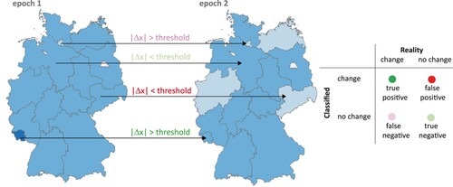
Much more elementary, however, is the problem that significant changes can be lost by data classification (referred to as change loss in the following) or non-significant changes can be unintentionally emphasized (change exaggeration). Avoiding these effects, which often work against each other (Figure 1), is of course a prerequisite for an effective detection of changes. Surprisingly, this topic has hardly or not at all been dealt with in the literature so far.

Figure 1. Problem setting: Fictional, bi-temporal dataset shown in arbitrary data classification; change event is based on comparison of value difference Δx between epochs and for each region with pre-defined threshold – leading to four exemplary cases of confusion matrix on the right (e.g. upper case reads: although threshold is exceeded, no change is shown in visualization  = = false negative).

The standard methods for data classification (such as equidistant or quantiles) determine the class boundaries based on the histogram along the number line, but change information as such is explicitly not considered and thus possibly lost.

Goal

The overall aim of this paper is to develop a classification method for multi-temporal data that reduces the described effects of change loss and exaggeration. Such a method must be able to handle different tasks concerning the value changes – e.g. the tasks of representing only the largest (highly significant) changes or all changes above a given threshold.

Optimizing the data classification for multi-temporal choropleth mapping needs to consider a careful definition of change tasks and a-priori temporal-thematic generalization operations. The resulting change loss or exaggeration effects have to be compared to existing methods using different preservation measures.

Outline

In the following, previous work on the basic problems of multitemporal choropleth maps and on task-oriented data classification is presented (Section 2). Section 3 describes the flexible data classification method, including the necessary preservation measures. The application of this method to typical datasets is demonstrated in Section 4, varying relevant parameters such as change task, number of epochs or number of classes. A discussion of transferability and parameter settings is given in Section 5. Finally, Section 6 summarizes the results and gives an outlook on future work.

Previous Work

Multi-temporal Choropleth Maps

Multi-temporal choropleth maps can basically appear in two forms – as cartographic animations or as static map series (in particular, small multiples). Cartographic animations gained prominence in the early 1990s, brought about by the increased power of computers, graphics cards, and so on (Campbell and Egbert, 1990; Peterson, 1995). Di Biase et al. (1992) provided a comprehensive overview on the design of such animations, while Blok (2000) described an assignment of appropriate dynamic visualization parameters to selected tasks. Cybulski (2022) stated that from a cartographic and psychological point of view there are still considerable deficits in describing the recognition of temporal trends of spatial patterns in animations. A comparison between animated maps with static map series is given, for example, in Griffin et al. (2006).

The effect of change blindness, i.e. the incomplete recognition of multi-temporal information due to the limited capacity of the human working memory, usually refers to the representation in cartographic animations. As an example, Rensink (2002) holds that a maximum of four to five elements can be perceived simultaneously. In a weakened form, however, the effect can also be transferred to static map series. There are numerous contributions in the literature that deal with this effect and the possible design causes for it (e.g. Harrower, 2007). The basic problem is that the number of visual stimuli is too large (i.e. the cognitive load is high). This can be caused in multi-temporal choropleth maps especially by large numbers of enumeration units, class values (and colours, respectively), epochs or change events as well as a high animation speed. In particular, simultaneous and opposite changes at different locations in the map are very difficult to capture. Another unwanted effect are false alarms: Users think they have detected colour changes, although they do not occur at all. This is often true for regions surrounded by regions with large changes (Cybulski and Krassanakis, 2021).

A number of graphical or interactive design measures are recommended to avoid change blindness. In particular, these include the integration of interactive elements for fast-forwarding and rewinding (e.g. through sliders; Harrower and Fabrikant, 2008). To avoid additional eye movements within a single time frame, alternative temporal legends are recommended – such as centring these legends or using speech or sound (Kraak et al., 1997; Muehlenhaus, 2013). Furthermore, the transition between frames can be varied: in so-called tweening, interpolation or smoothing takes place between map frames of an animation, thereby extending the respective display duration. Whereas Fish et al. (2011) found that this measure actually improved readability, Simons (2000) detected underestimations of large changes due to tweening and recommended abrupt changes for this purpose.

As an alternative or addition to the aforementioned design measures, there is also the possibility of reducing the problem of change blindness by a priori data transformation or data generalization – this can refer to both spatial and temporal dimensions (Panopoulos et al., 2003). Typical examples for the latter dimension are temporal selection (of specific epochs), aggregation (e.g. building monthly average of daily values) or smoothing (e.g. of daily data with 5-day windows by averaging values of four days before and the current day). Harrower (2001) recommended temporal smoothing; however, McCabe (2009) and Traun et al. (2021) found no improved perception through this approach. Traun et al. (2021) successfully performed a generalization that excluded local outliers. Traun and Mayrhofer (2018) reduced visual complexity in advance by a generalization based on spatiotemporal autocorrelation that eliminates ‘visual noise’, thus preserving both large-scale patterns and local variations. In general, data generalization also causes loss of information or misinterpretation of data; for example, Becontyé et al. (2022) investigated the effect of different levels of aggregation in choropleth maps. Any data classification has to be treated separately for individual applications – an example of processing COVID-19 datasets is given by Halpern et al. (2021).

Task-oriented Data Classification

The topic of data classification for cartographic purposes is treated extensively in the literature – here one can refer to the overview contributions of Cromley and Cromley (1996) or Coulsen (1987). The clear focus is on data-driven methods for static displays. It is therefore not surprising that only methods of this kind are implemented in common GIS or mapping software. In addition, interactive tools have been developed to find the ‘optimal’ configuration for a given application; e.g. the use of linked views between data histogram and choropleth map (Andrienko et al., 2001).

Focusing on the spatial component only, the task to preserve spatial patterns in mono-temporal maps can be seen as a somehow similar problem to the one tackled in this paper. Common data-driven methods do not guarantee the preservation, so that in practice the typical case is a manual subjective selection from several created variants. An overview of task-oriented approaches to address this problem is given by Armstrong et al. (2003). Often, the goal is to simplify the displayed patterns so that the map user can more quickly grasp the broad trends in the display without being disturbed by a detailed and ‘spotty’ impression (Cromley, 1996; Andrienko et al., 2001; Slocum et al., 2009). However, this approach does not guarantee that any significant pattern that may be present is preserved. Hence, Chang and Schiewe (2018) developed methods to preserve specific patterns such as the detection of differences in values between polygons, hot and cold spots, global or local extreme values, or cluster regions.

A specific treatment of multi-temporal data classification is hardly done in the literature. One of the few exceptions is the work of Monmonier (1994), which aimed at minimizing small or unwanted class changes (but did not lead to satisfying results either). Harrower (2003) recommended a strong aggregation into two or three classes, which is, however, an overly simplified option for many applications.

Brewer and Pickle (2002) suggested that – applying different existing classification methods – quantiles showed best results for map comparison purposes. However, they tested only a three-class variant and found that many undesired class breaks occurred between same values so that a a-posteriori adjustment was applied. Different change tasks were not taken into consideration; for example, the quantile method will be optimal to represent only very few, largest changes. The authors also experienced that matched legends across all epochs of the time series increased the map comparison accuracy significantly (by 28 percent).

Summarizing these findings, on can state that the impact of change loss and change exaggeration in the course of data classification is rarely, if ever, discussed in the literature. On the other hand, however, this aspect should represent a fundamental basis on which further improvements for the perceptibility of changes in choropleth maps can then be developed. Simply speaking, if the aim is to detect changes, they should remain visible after data classification.

There are, of course, empirical findings for selecting appropriate classification methods for mono-temporal scenes that can consider, for example, known data distributions (e.g. the pre-knowledge that equidistant distributions are not suitable for strongly skewed distributions such as the population density in Germany or in other countries). On the other hand, a dataset for multi-temporal scenes is now extended even further by the fact that very many and different changes occur – and with that a proper assignment of a known classification method is usually not possible.

Method

In order to find an appropriate, task-oriented visualization format for multi-temporal choropleth maps, firstly the desired change task should be defined as clear as possible. The next section describes measures for the impact of data classification on change preservation. These measures are then used to control a new data classification algorithm.

Change Tasks

The definition of the change task includes the selection of epochs, i.e. the first and last epoch as well as the temporal resolution. The definition of temporal resolution can be based on a predefined temporal lag (e.g. considering only dates with a lag of two months) or on thematic relevance (e.g. considering only the summer months for vegetation applications).

Depending on the application, but also on the information content of the data, a user is interested in very different types of changes. If we first look at the values x_t1 and x_t2 for two lags at a certain enumeration unit, we can differentiate local changes such as:

• simple value changes (i.e. |Δx| = |x_t1 - x_t2| > 0 between lags),

• significant value change (i.e. |Δx| > given threshold, based on statistical analysis, and so on),

• change in tendency (e.g. increase, constant, decrease),

• epoch of first/last (significant) change (appearance, decay),

• epochs of all (significant) changes,

• (maximum, minimum) duration of all (significant) changes.

Of course, combinations of these types are also possible. If not only one enumeration unit at a time is considered, changes in patterns may also be of interest, such as growth or shrinkage of clusters or hot/cold spots (focal or global changes). In the remainder of this paper, however, we will focus on local changes only.

Based on the desired type of local changes, appropriate mathematical, statistical or application-oriented measures of changes have to be introduced. Possible measures are:

• (Absolute) difference between values of two different epochs of time (Δx = x_t1 - x_t2; or |Δx|),

• (absolute) quotient of values of two different epochs of time (x_t1 / x_t2; or |x_t1 / x_t2|),

• (absolute) difference between values and trend for one location at given epoch (the trend might be derived from temporal smoothing of the time series).

Preservation of Changes (POCC)

Change of Values and Classes

The general task of mono-temporal data classification is to assign class values c (c = 1,..,k; c∈N) to given attribute values x (x = x_MIN,..,x_MAX; x∈R). The class assignment can be described in a general manner as follows: (1) $c=\{\begin{array}{c}1forx\le x_1\\ 2forx>x_{1}ANDx\le x_2\\ (\dots )\end{array}$(1) Hence, the task is to determine the class limits x_i (i = 1,..k). As an example, for the equidistant method the following condition has to be fulfilled: (2) $x_2-x_1=x_3-x_2=\dots$(2)

In the case of multi-temporal datasets, i.e. with data for given epochs t (t = 1,..,n), the formulation of the task has to be extended: For given attribute values at a enumeration unit at time t (x_t; x ∈R) respective class values c (c∈N) are required. It is assumed that there is one common classification scheme for all epochs of the time series in order to ensure comparability (Brewer and Pickle, 2002).

With that one also obtains class (or rank) differences Δc for given value differences Δx between two epochs. The overall aim is to define a set of class breaks that is able to preserve as many significant value differences (for example, to avoid change loss for large differences), and/or to avoid class breaks between very small changes (i.e. to avoid change exaggeration).

When transforming given value differences Δx into required class differences Δc_required several approaches are conceivable depending on the change task. The evaluation of the preservation can be done via different measures.

Selected Variants

When transforming given value differences Δx into required class differences Δc_required, several approaches are conceivable depending on a certain change task. In the following, three important variants are presented as examples, which describe an upper threshold value Δx_UPPER for the class with the ‘most important’ changes. The classification of the remaining change values is done in different ways (Figure 2). The definition of the necessary threshold values is for example based on statistical parameters (e.g. using 2σ-, 1σ-, etc. values, or any percentiles) or by taking application-dependent definitions of ‘important changes’ into consideration.

Figure 2. Variants of the assignment of class differences Δc depending on value differences Δx. Δx_MIN and Δx_MAX are the extreme value changes within dataset; the other thresholds are determined based on variants as described in the text.

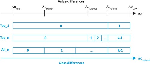
With the ‘Top_1’ variant, all changes Δx above a threshold value Δx_UPPER receive a class difference Δc_required = 1: (3) $\mathrm{\Delta }{c}_{required}=1for|\mathrm{\Delta }x|>\mathrm{\Delta }{x}_{UPPER}$(3)

Δx_UPPER can be defined, for example, using a quantile of the entire dataset (e.g. the 90% quantile). If Δx_UPPER = Δx_MAX were set, only this maximum difference would be included in the top class change class.

With the variant ‘Top_n’, all changes Δx above a threshold value Δx_MIDDLE are transferred into several, equally spaced class jumps. Again, the top class starts at the threshold value Δx_UPPER. If the classification is calculated for k classes, the required class difference is given by: (4) $\mathrm{\Delta }{c}_{required}=\left\{\begin{array}{c}INT\left({\displaystyle \frac{k-2}{\mathrm{\Delta }{x}_{UPPER}-\mathrm{\Delta }{x}_{MIDDLE}}(\mathrm{\Delta }\mathrm{x}-\mathrm{\Delta }{x}_{MIDDLE})+1}\right)for\mathrm{\Delta }x>\mathrm{\Delta }{x}_{MIDDLE}\\ 0else\end{array}\right\}$(4) Both Δx_MIDDLE and Δx_UPPER can be set, for example, by using quantiles of the entire dataset (e.g. the 70% and 90% quantiles).

With the ‘All_n’ method, all changes Δx above a threshold value Δx_LOWER are transformed into several, equally spaced class differences. The top class starts at the threshold value Δx_UPPER. If the classification is calculated for k classes, the required class difference as a special case of ‘Top-n’ (with Δx_LOWER= 0) results from (5) $\mathrm{\Delta }{c}_{required}=INT\left({\displaystyle \frac{k-1}{\mathrm{\Delta }{x}_{UPPER}}\mathrm{\Delta }x}\right)$(5)

Evaluation of Preservation

After applying any data classification method, the requested class differences Δc_required can be compared with the differences Δc_achieved that have actually been obtained. For that purpose, simply the absolute or relative number of preserved change classes could be counted. A more meaningful measure is based on the metrics as introduced by Goldsberry and Battersby (2009). They counted either the number of enumeration units whose class changed (somehow) between two epochs (Basic Magnitude of Change; BMOC), or the total number of cardinal or ordinal classes that changed between two epochs, also taking into account the magnitude of the possible class difference (Magnitude Of Rank Change; MORC). Figure 3 demonstrates the respective weighting factors for the BMOC- and MORC-measures (for an example with three classes).

Figure 3. Comparison of weights for measures BMOC and MORC (according to Goldsberry and Battersby, 2009) and for measure POCC (including weights w – see text below).

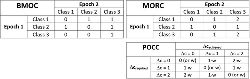
In contrast to Goldsberry and Battersby (2009), in this contribution we do not consider the change of values x, but the preservation of change classes (POCC) Δc. To do this, the number of required class differences for a given value interval (Δc_required) is compared to the actual class interval achieved by data classification (Δc_achieved; Figure 3). A normalization is realized by dividing this difference by Δc_required, resulting in the following POCC measure: (6) $POCC=1-{\displaystyle \frac{{\sum }_i{w}_i\cdot |\mathrm{\Delta }{c}_{required,i}-\mathrm{\Delta }{c}_{achieved,i}|}{{\sum }_i{w}_i\cdot \mathrm{\Delta }{c}_{required,i}}}$(6) The index i runs over all pairs of values with a predefined lag (by default lag = 1, i.e. consecutive pairs). The larger POCC (with maximum 1), the better the preservation. The weights w can be used to emphasise certain class preservations. In the ‘Top_1’ variant, the weights w are set as follows: (7) $w_i=\{\begin{array}{c}1for\mathrm{\Delta }{c}_{required}=1\\ 0else\end{array}$(7)

In contrast, for variants ‘Top_n’ and ‘All_n’ the weights are set as follows: (8) $w_i=\mathrm{\Delta }{c}_{required}$(8) The differences between Δc_required and Δc_achieved in POCC consider false negatives (i.e. change loss). By introducing a weighting of the no-change classes (Δc_required= 0), however, the false positives (i.e. change exaggeration) can also be considered – for the variant ‘Top_1’ by setting for all differences (9) $w_i=1$(9) as well as for variants “Top_n” and “All_n” by: (10) $w_i=\{\begin{array}{c}k-1for\mathrm{\Delta }{c}_{required}=0\\ \mathrm{\Delta }{c}_{required}else\end{array}$(10) Alternatively, the false positives can also be described by their relative number directly – either in comparison to the total number of all changes (FP1), or in comparison to the number of all Δc_required> 0 (FP2). In general, the larger FP1 or FP2 are, the larger the proportion of unwanted false positives. If, for example, FP2 > 1, more than half of all class changes are not due to requested changes at all and thus do not allow the isolated detection of significant changes.

Grouping into classes generally leads to a loss of original values. In order to determine the degree of these losses (also in comparison to other methods), the simple measure Preservation of Original Values (POOV) is used in the following. For this purpose, the dispersion of the original values x is determined for each epoch by means of the standard deviation (RMSE_x). This value is divided by the predefined width of equidistant of classes (Δx_equidistant), which corresponds to the standard deviation of a corresponding equidistant grouping. This reference value is compared to the standard deviation of the class values (RMSE_Class) for each epoch in the (POCC or any other) classification: (11) $POOV=1-{\displaystyle \frac{1}{n}\sum _{t=1}^n\left|{\displaystyle \frac{RMS{E}_x}{\mathrm{\Delta }{x}_{equidistant}}-RMS{E}_{Class}}\right|}$(11) The larger POOV (with the maximum POOV = 1), the better the dispersion of the original values is preserved after classification.

POCC Data Classification

The determination of class limits for given attribute values x, which also considers the aforementioned determined required change classes Δc_required, is performed through a sweep line algorithm. The corresponding diagram (Figure 4) shows attribute values x on the right axis, while all attribute differences Δx between two lags are plotted as intervals below. These differences are already grouped according to the respective required class difference Δc_required.

Figure 4. Sweep line diagram for given dataset: line segments below number line (representing values x) show placement and length of all value intervals |Δx|. This arbitrary example for variant ‘All_n’ requires class differences Δc (shown on right hand side) for ΔxUPPER = 60 and ΔxLOWER = 20.

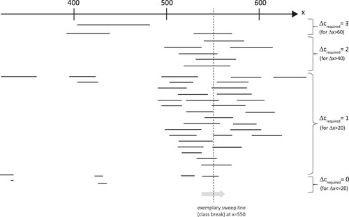
The sweep line is moved from left to right over the intervals. For this purpose, discrete steps must be defined for the sweep line based on the properties of the dataset and the resulting computation time. The strictest option is to choose this resolution smaller than the smallest difference between the values x occurring in the dataset.

An intersection of a sweep line with such an interval represents a possible class boundary between the lower and upper breaks of the interval. For each sweep line, the corresponding number of intersections with value intervals |Δx| can be counted. At the end, for each interval the total number of intersections (i.e. the class difference Δc_achieved) is counted and compared to the required value Δc_required using the POCC measure (section 3.2.3).

Given an a priori fixed number of change classes, the optimal solution is obtained using a brute force approach that considers all possible combinations of sweep lines (i.e. all class boundaries) and the respective preservation measures POCC. The best combination is then selected based on the maximum POCC value. In the following, this novel method will also be referred as POCC data classification method.

Example

Dataset

The Robert Koch Institute (Berlin, Germany) continuously publishes various spatiotemporal data on COVID-19 cases on its website. In the following, the dataset for daily calculated 7-day incidences for each of the 16 federal states in Germany is used (between 11th September 2021 and 17th April 2023).

To reduce this dataset, temporal aggregation was performed – a maximum of 19 epochs were thus generated by monthly averaging. For comparison purposes, also subsets with four epochs (Figure 5) and six epochs were created.

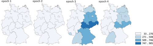
Figure 5. Example dataset on monthly COVID-19 incidences – four epochs, equidistant classification with four classes (data source: https://www.rki.de/DE/Content/InfAZ/N/Neuartiges_Coronavirus/Daten/Inzidenz-Tabellen.html).

POCC Classification

The POCC data classification described above was performed for all combination of the following parameter variations:

• POCC-Variants: ‘Top_1’, ‘Top_n’ and ‘All_n’;

• Number of classes: 3, 4 and 5. As stated above, Harrower (2003) recommended a strong aggregation into two or three classes; however, this overly simplified option is extended to more typical values for cartographic animations;

• Number of epochs: 4, 6 and 19.

The absolute difference |Δx| was used as a measure of the change between two epochs. To determine the threshold values, Δx_UPPER was equated with the 90% quantile and Δx_MIDDLE with the 70% quantile of the dataset.

The evaluation is carried out using the measures listed above (POCC, POOV, FP1, FP2). For comparison purposes, the corresponding measures for the equidistant classification method were also determined. Tables 1–4 summarise the results, sorted by the variants ‘Top_1’, ‘Top_n’ and ‘All_n’ (the latter with the different weighting methods). Parallel to these tables, Figures 6–9 show an example of the resulting choropleth map series for one case (four epochs, four classes). In the figures, the assignment of true/false and positive/negative is marked, independent of the magnitude of the required class difference.

Figure 6. POCC classification for variant ‘Top_1’ (four epochs, four classes), point symbols describe correctness of change relative to previous epoch.

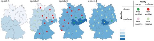
Figure 7. POCC classification for variant ‘Top_n’.

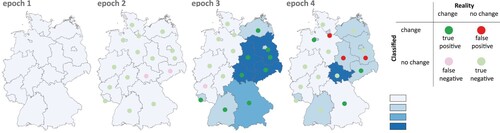
Figure 8. POCC classification for variant ‘All-n’ (no weighting for no-class changes).

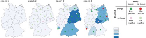
Figure 9. POCC classification for variant ‘All-n’ (with weighting for no-class changes).

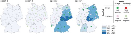
Table 1. Results of variant ‘Top_1’ ($w_i=\mathrm{\Delta }{c}_{required}$).

Epochs	Classes	Class breaks POCC	POCC		POOV		FP1		FP2
			POCC	equi	POOC	equi	POCC	equi	POCC	equi
4	3	130/607	1.00	.60	.76	.87	.29	.21	2.80	2.00
	4	54/130/608	1.00	−.20	.60	.92	.38	.29	3.60	2.80
	5	54/68/130/608	1.00	−.40	.40	.94	.33	.33	3.20	3.20
6	3	535/1557	1.00	.50	.89	.95	.24	.31	2.38	3.13
	4	54/535/1557	1.00	−.25	.76	.91	.31	.35	3.13	3.50
	5	54/68/535/1557	1.00	−.88	.62	.91	.39	.38	3.88	3.75
19	3	514/1557	1.00	.50	.23	.39	.32	.20	15.33	9.67
	4	23/514/1557	1.00	.00	.08	.16	.32	.35	15.33	16.67

Table 4. Results of variant ‘All_n’ (with weighting for no-class changes).

Epochs	Classes	Class breaks POCC	POCC		POOV		FP1		FP2
			POCC	equi	POCC	equi	POCC	equi	POCC	equi
4	3	253/457	.69	.50	.82	.87	.08	.02	.33	.05
	4	262/403/634	.67	.54	.57	.92	.00	.04	.00	.09
	5	253/262/403/536	.68	.45	.60	.94	.04	.00	.09	.00
6	3	641/1044	.73	.63	.89	.96	.04	.04	.10	.08
	4	457/641/946	.74	.63	.82	.91	.05	.01	.11	.02
	5	457/641/874/1044	.74	.60	.86	.85	.04	.00	.07	.00
19	3	1040/1670	.29	−.25	.55	.50	.04	.03	.38	.11
	4	665/1044/1404	.66	.29	.40	.35	.05	.06	.16	.18

Discussion

The following discussion evaluates the POCC data classification based on the introduced measures – namely, preservation of class changes (POCC), preservation of dispersion of input data (POOV) and the relative number of false positives (FP1 and FP2).

With regard to the preservation of desired class changes, the expected ‘superiority’ of the POCC over the equidistant classification becomes apparent for all variants. This is logical insofar as the classification is controlled according to the POCC criterion. Nevertheless, it is striking that the equidistant method never reaches this optimal value of preservation.

If one looks at the behaviour of the POCC value as a function of the number of classes, there is no clear tendency. For the variants ‘Top_n’ and ‘All_n’ (Tables 2 and 3), at best a slight decrease can be observed as the number of classes increases. There is also no clear dependence on the number of epochs. There are hardly any differences between the variants ‘Top_n’ and ‘All_n’ (the latter without weighting of the no-changes). However, there are significantly worse values for ‘All_n’ with weighting of the no-changes (Table 4), since a larger number of potential misclassifications are added by the no-change class and thus worsen the POCC value. In contrast, the number of cases considered is significantly lower for the variant ‘Top_1’, which leads to 100% preservation in the given example.

Table 2. Results of variant “Top_n” ($w_i=\mathrm{\Delta }{c}_{required}$).

Epochs	Classes	Class breaks POCC	POCC		POOV		FP1		FP2
			POCC	equi	POCC	equi	POCC	equi	POCC	equi
4	3	262/565	.82	.61	.87	.87	.06	.06	.20	.20
	4	262/536/565	.71	.61	.78	.92	.02	.13	.07	.40
	5	251/339/536/565	.70	.50	.72	.94	.10	.17	.33	.53
6	3	641/946	.79	.70	.87	.95	.25	.11	.83	.38
	4	457/641/946	.68	.58	.82	.91	.34	.15	1.12	.50
	5	641/714/874/936	.62	.48	.72	.84	.22	.15	.75	.50
19	3	614/1285	.84	.79	.36	.46	.17	.09	1.20	.68
	4	726/1040/1748	.81	.73	.39	.24	.11	.23	.82	1.65

Table 3. Results of variant ‘All_n’ (no weighting for no-class changes).

Epochs	Classes	Class breaks POCC	POCC		POOV		FP1		FP2
			POCC	equi	POOV	equi	POCC	equi	POCC	equi
4	3	262/565	.84	.62	.87	.87	.06	.02	.25	.05
	4	262/339/565	.73	.63	.52	.92	.05	.04	.08	.09
	5	262/268/403/565	.72	.49	.60	.94	.02	.00	.04	.00
6	3	427/946	.87	.77	.89	.96	.06	.04	.16	.08
	4	427/641/946	.78	.65	.84	.91	.04	.01	.08	.02
	5	427/641/874/1044	.76	.63	.88	.85	.04	.00	.07	.00
19	3	614/1285	.84	.80	.35	.50	.18	.03	1.38	.11
	4	514/972/1404	.85	.82	.26	.35	.14	.06	.52	.18

When looking at the preservation of the dispersion of the input data, it becomes apparent that the POCC classification usually has quite similar, but usually slightly worse values compared to the equidistant classification. Of course, it is debatable how much the dispersion behaviour should be preserved at all, since this can compete with the highlighting of the class changes and large dispersions can rather lead to many class changes and confusion for the user. However, it can be stated that the POCC classification does not cause any significant loss of the original input data.

As already mentioned, the focus of the POCC measure is on the consideration of false negatives, i.e. those desired class changes that are not produced by a classification (i.e. change loss). On the other hand, however, false positives (FP) also significantly interfere with the interpretation of a visualization, as these unintended class changes (i.e. change exaggeration) cannot be separated from the intended changes.

The POCC measure offers a consideration through appropriate weighting – as for the variant ‘All_n’ with the weight w = k-1 for the consideration of no-changes (Table 4). As expected, the POCC numbers are reduced by this stricter measure compared to the ‘All_n’ variant without weighting of the no-changes (Table 3).

Conversely, the measures FP1 and FP2 directly show the relative proportions of false positives. Here, the elementary weakness of the ‘Top_1’ variant (Table 1) becomes quite clear: relatively large changes receive a class difference of 1 – but such a difference also occurs relatively frequently with smaller value differences due to the value distribution at the selected boundaries. In particular, the measure FP2 shows that the number of class differences due to relatively small differences is a multiple (by factors of 3.6 to 6.0) of the intended class differences (above the threshold Δx_UPPER), which means that the intended detection of larger differences only is not possible.

For the other variants, there is no clear dependence of FP1 and FP2 on the number of classes or epochs. There is also no clear tendency towards the equidistant classification, which indicates random deviations depending on the real data distribution. In summary, it can be stated that the POCC classification shows neither advantages nor disadvantages with regard to the false positives compared to the equidistant classification – which is not surprising in view of the explicit non-consideration (except for the weighting of the no-changes for ‘All_n’).

Summary and Outlook

Summary

In this paper, a novel extended method for data classification was presented, which explicitly considers the most complete preservation of ‘important’ and/or the avoidance of ‘unimportant’ class changes – and thus reduces the effects of change loss or change exaggeration. For this purpose, the measure POCC was introduced, which is able to control and optimize this procedure. By introducing different weights, certain change types (e.g. the highest change values) can be emphasized.

The behaviour of the measures POCC for the preservation of class changes showed the added value compared to the equidistant classification, while there were no significant deviations regarding the preservation of the original dispersion in the dataset as well as the relative number of false positives. With that, the overall aim of this paper could be fulfilled, which was the development of a classification method for multi-temporal data that reduces the effects of change loss and exaggeration and allows the consideration of different change tasks.

Future Work

With respect to the POCC data classification algorithm some further developments are conceivable, for example:

• An essential extension should include the consideration or avoidance of the significantly disturbing false positives – beyond the previously introduced, optional weighting of the no-changes in the POCC measure.

• So far, once thresholds have been set (Δx_UPPER, and if needed also Δx_MIDDLE, Δx_LOWER), a proportional classification of classes in the remaining range of values has been assumed. It is conceivable that additional criteria could be used to achieve better preservation measures for non-proportional class ranges.

• In this paper, local significant value changes (described by the absolute difference |Δx|) were used as the change type. Although this can certainly be seen as the most important change type, other types (such as deviation from trend) and other measures (such as quotient) must be considered, leading to adopted definitions of the POCC measure.

• The POCC measure was used as a global measure so far – depending on the application or distribution of the data, local weighting is also conceivable.

• A disadvantage of the previous implementation is the brute force approach, which sometimes leads to long calculation times (which was one of the reasons for not calculating the option ‘19 epochs/5 classes’ which takes many hours using an standard computer). Optimizations and approximations are necessary here.

From a methodological point of view, it should be noted that the experimental verification has so far only been carried out with one dataset. With the help of the different number of epochs, a certain variance of input values x as well as of changes Δx has already been achieved – nevertheless, further sample data are still to be examined. In this context, alternative threshold values should also be used (instead of Δx_UPPER = 90% quantile or Δx_MIDDLE= 70% quantile in this contribution).

Empirical studies will help to describe the influence and sensitivity of different parameter settings on the changes actually perceived by the user. In other words, it has to be examined whether the numerical progress as achieved with POCC classification is actually perceived by users. In this context, different types of multi-temporal visualizations (namely, cartographic animations and small multiples) have to be differentiated in future investigations.

Code Availability

The core code for POCC classification (usable for different variants) is stored at https://github.com/luftj/pocc

Acknowledgements

The author thanks M.Sc. Jonas Luft for code implementation.

Disclosure Statement

No potential conflict of interest was reported by the author(s).

Data Availability Statement

Data used in the experiments were extracted from https://www.rki.de/DE/Content/InfAZ/N/Neuartiges_Coronavirus/Daten/Inzidenz-Tabellen.html

Additional information

Notes on contributors

Jochen Schiewe

Jochen Schiewe is Full Professor for Geoinformatics and Geovisualization at HafenCity University Hamburg, Germany. His works are mainly concerned with the development of task-oriented algorithms in cartography and the modelling and visualization of uncertainties in geo data. He is President of the German Cartographic Society (DGfK).

References

- Andrienko, G., Andrienko, N. and Savinov, A. (2001) “Choropleth Maps: Classification Revisited” Proceedings of the International Cartographic Conference Beijing, China: 6th–10th August, p.9.
- Armstrong, M.P., Xiao, N. and Bennett, D.A. (2003) “Using Genetic Algorithms to Create Multicriteria Class Intervals for Choropleth Maps” Annals of the Association of American Geographers 93 (3) pp.595–623 DOI: 10.1111/1467-8306.9303005.
- Beconytė, G., Balčiūnas, A., Šturaitė, A. and Viliuvienė, R. (2022) “Where Maps Lie: Visualization of Perceptual Fallacy in Choropleth Maps at Different Levels of Aggregation” ISPRS International Journal of Geo-Information 11 (1) p.64 DOI: 10.3390/ijgi11010064.
- Bill, R., Blankenbach, J., Breunig, M., Haunert, J.-H., Heipke, C., Herle, S., Maas, H.-G., Mayer, H., Meng, L., Rottensteiner, F., Schiewe, J., Sester, M., Sörgel, U. and Werner, M. (2022) “Geospatial Information Research: State of the Art, Case Studies and Future Perspectives” Journal of Photogrammetry, Remote Sensing and Geoinformation Science 90 (4) pp.349–389 DOI: 10.1007/s41064-022-00217-9.
- Blok, C. (2000) “Monitoring Change: Characteristics of Dynamic Geo-Spatial Phenomena for Visual Exploration” In Freksa, C., Habel, C., Brauer, W. and Wender, K.F. (Eds) Spatial Cognition II. Lecture Notes in Computer Science, Vol. 1849 pp.16–30. Berlin, Heidelberg: Springer DOI: 10.1007/3-540-45460-8_2.
- Brewer, C.A. and Pickle, L. (2002) “Evaluation of Methods for Classifying Epidemiological Data on Choropleth Maps in Series” Annals of the Association of American Geographers 92 (4) pp.662–681.
- Campbell, C.S. and Egbert, S.L. (1990) “Animated Cartography: Thirty Years of Scratching the Surface” Cartographica 27 (2) pp.24–46.
- Chang, J. and Schiewe, J. (2018) “An Open Source Tool for Preserving Local Extreme Values and Hot/Coldspots in Choropleth Maps” Kartographische Nachrichten 68 (6) pp.307–309 DOI: 10.1007/BF03544625.
- Coulsen, M.R.C. (1987) “In the Matter of Class Intervals for Choropleth Maps: With Particular Reference to the Work of George Jenks” Cartographica 24 (2) pp.16–39 DOI: 10.3138/U7X0-1836-5715-3546.
- Cromley, R.G. (1996) “A Comparison of Optimal Classification Strategies for Choroplethic Displays of Spatially Aggregated Data” International Journal of Geographical Information Systems 10 (4) pp.405–424 DOI: 10.1080/02693799608902087.
- Cromley, E.K. and Cromley, R.G. (1996) “An Analysis of Alternative Classification Scheme for Medical Atlas Mapping” European Journal of Cancer 32 (9) pp.1551–1559 DOI: 10.1016/0959-8049(96)00130-X.
- Cybulski, P. (2022) “An Empirical Study on the Effects of Temporal Trends in Spatial Patterns on Animated Choropleth Maps” ISPRS International Journal of Geo-Information 11 (5) p.273 DOI: 10.3390/ijgi11050273.
- Cybulski, P. and Krassanakis, V. (2021) “The Role of Magnitude of Change in Detecting Fixed Enumeration Units on Dynamic Choropleth Maps” The Cartographic Journal 58 (3) pp.251–267 DOI: 10.1080/00087041.2020.1842146.
- DiBiase, D., MacEachren, A.M., Krygier, J.B. and Reeves, C. (1992) “Animation and the Role of Map Design in Scientific Visualization” Cartography and Geographic Information Systems 19 (4) pp.201–214 DOI: 10.1559/152304092783721295.
- Fish, C., Goldsberry, K.P. and Battersby, S. (2011) “Change Blindness in Animated Choropleth Maps: An Empirical Study” Cartography and Geographic Information Science 38 (4) pp.350–362 DOI: 10.1559/15230406384350.
- Goldsberry, K. and Battersby, S. (2009) “Issues of Change Detection in Animated Choropleth Maps” Cartographica 44 (3) pp.201–215 DOI: 10.3138/carto.44.3.201.
- Griffin, A.L., MacEachren, A.M., Hardisty, F., Steiner, E. and Li, B. (2006) “A Comparison of Animated Maps with Static Small-Multiple Maps for Visually Identifying Space-Time Clusters” Annals of the Association of American Geographers 96 (4) pp.740–753 DOI: 10.1111/j.1467-8306.2006.00514.x.
- Halpern, D., Lin, Q., Wang, R., Yang, S., Goldstein, S. and Kolak, M. (2021) “Dimensions of Uncertainty: A Spatiotemporal Review of Five COVID-19 Datasets” Cartography and Geographic Information Science pp.1–22 DOI: 10.1080/15230406.2021.1975311.
- Harrower, M. (2001) “Visualizing Change: Using Cartographic Animation to Explore Remotely-Sensed Data” Cartographic Perspectives 39 pp. 30–42 DOI: 10.14714/CP39.637.
- Harrower, M. (2003) “Tips for Designing Effective Animated Maps” Cartographic Perspectives (44) pp.63–65 DOI: 10.14714/CP44.516.
- Harrower, M. (2007) “The Cognitive Limits of Animated Maps” Cartographica 42 (4) pp.349–357 DOI: 10.3138/carto.42.4.349.
- Harrower, M. and Fabrikant, S.I. (2008) “The Role of Map Animation for Geographic Visualization” In Dodge, M., Derby, M. and Turner, M. (Eds) Geographic Visualization: Concepts, Tools and Applications Chichester: John Wiley & Sons, pp.49–65.
- Jenks, G.F. (1977) “Optimal Data Classification for Choropleth Maps” (Occasional Paper No. 2) Department of Geography, Q2 University of Kansas.
- Kraak, M.-J., Edsall, R. and MacEachren, A.M (1997) “Cartographic Animation and Legends for Temporal Maps: Exploration and or Interaction” Proceedings of the 18th International Cartographic Conference, Stockholm, Sweden: 23rd–27th June, pp.253–261.
- McCabe, C.A. (2009) “Effects of Data Complexity and Map Abstraction on the Perception of Patterns in Infectious Disease Animations” (Master’s Thesis). Pennsylvania State University, University.
- Meng, L. (2020) “An IEEE Value Loop of Human-Technology Collaboration in Geospatial Information Science” Geo-spatial Information Science 23 (1) pp.61–67 DOI: 10.1080/10095020.2020.1718004.
- Monmonier, M. (1994) “Minimum-change Categories for Dynamic Temporal Choropleth Maps” Journal of the Pennsylvania Academy of Science 68 (1) pp.42–47.
- Mooney, P. and Juhász, L. (2020) “Mapping COVID-19: How Web-Based Maps Contribute to the Infodemic” Dialogues in Human Geography 10 (2) pp.265–270 DOI: 10.1177/2043820620934926.
- Muehlenhaus, I. (2013) Web Cartography: Map Design for Interactive and Mobile Devices Boca Raton, FL: CRC Press.
- Panopoulos, G., Stamatopoulos, A. and Kavouras, M. (2003): Spatio-temporal Generalization: The Chronograph Application Proceedings of the 21st International Cartographic Conference, Durban, South Africa Available at: https://icaci.org/files/documents/ICC_proceedings/ICC2003/Papers/256.pdf.
- Peterson, M.P. (1995) Interactive and Animated Cartography Englewood Cliffs, NJ: Prentice Hall.
- Rensink, R.A. (2002) “Internal vs. External Information in Visual Perception” Proceedings of the 2nd International Symposium on Smart Graphics – SMARTGRAPH ‘02, Hawthorne, NY: 11th–13th June: ACM Press, pp.63–70.
- Rezk, A.A. and Hendawy, M. (2023) “Informative Cartographic Communication: A Framework to Evaluate the Effects of Map Types on Users’ Interpretation of COVID-19 Geovisualizations” Cartography and Geographic Information Science, pp.1–18 DOI: 10.1080/15230406.2022.2155249.
- Simons, D.J. (2000) “Attentional Capture and Inattentional Blindness” Trends in Cognitive Sciences 4 (4) pp.147–155 DOI: 10.1016/S1364-6613(00)01455-8.
- Slocum, T.A., McMaster, R.B., Kessler, F.C. and Howard, H.H. (2009) Thematic Cartography and Geovisualization (3rd ed.). Upper Saddle River, NJ: Prentice Hall.
- Sun, M., Wong, D. and Kronenfeld, B. (2017) “A Heuristic Multi-Criteria Classification Approach Incorporating Data Quality Information for Choropleth Mapping” Cartography and Geographic Information Science 44 (3) pp.246–258 DOI: 10.1080/15230406.2016.1145072.
- Traun, C. and Mayrhofer, C. (2018) “Complexity Reduction in Choropleth Map Animations by Autocorrelation Weighted Generalization of Time-Series Data” Cartography and Geographic Information Science 45 (3) pp.221–237 DOI: 10.1080/15230406.2017.1308836.
- Traun, C., Schreyer, M.L. and Wallentin, G. (2021) “Empirical Insight from a Study on Outlier Preserving Value Generalization in Animated Choropleth Maps” ISPRS International Journal of Geo-Information 10 (4) p.208 DOI: 10.3390/ijgi10040208.