Everybody herds, sometimes: cumulative advantage as a product of rational learning

Abstract

We propose a model of cumulative advantage (CA) as an unintended consequence of the choices of a population of individuals. Each individual searches for a high quality object from a set comprising high and low quality objects. Individuals rationally learn from their own experience with objects (reinforcement learning) and from the observation of others’ choices (social learning). We show that CA emerges inexorably as individuals rely more on social learning and as they learn from more rather than fewer others. Our theory argues that CA has social dilemma features: the benefits of CA could be enjoyed with modest drawbacks provided individuals would practice restraint in their social learning. However, when practiced by everyone such restraint goes against the individual’s self-interest.

1. Introduction

Every day, individuals and organizations must choose between alternatives, such as which music to buy, which restaurant to visit, or which law firm to hire. Although many of these decisions are routine, involving low stakes and little uncertainty about the quality of the alternatives, the stakes can be high and differences in quality of alternatives are not always evident (Strang & Macy, 2001). For instance, when commuters make decisions about which car to purchase, or organizations decide which law firm to contract for representation, it is important that they choose (one of) the best from a set of alternatives. While success in picking the best alternative is paramount, the quality of alternatives is at least partially hidden.

In making choices under conditions of uncertainty, choosers generally draw on two sources of information about the quality of alternatives: their own previous experiences and their observations of the choices others have made in the same domain. While experiential learning is typically the most informative of the quality of a given alternative, it is relatively slow and entails high search costs (cf. Stigler, 1961), requiring choosers to cycle through many low-quality alternatives before finding a high quality one. Social learning can be much faster, as it provides access to quality information about many alternatives simultaneously. But it is also riskier, since the behaviors of others may imperfectly reflect the quality of alternatives (cf. Anderson & Holt, 1997; Berger et al., 2018). As we show in this paper, how experiential and social learning contribute to the behaviors of a population of choosers has important implications for i) the success of individual choosers in finding the best alternative, ii) the number of choosers an alternative attracts, and iii) overall population inequality.

In an ideal and equitable world, learning through experience or observation would infallibly and quickly guide choosers to a best alternative, and alternatives would attract choosers in proportion to their relative quality. But the world is often inefficient, inequitable or both. For instance, empirical research shows clear evidence of herding, with all choosers converging on a single lower quality alternative (Bikhchandani et al., 1992; Raafat et al., 2009; Trueman, 1994). Relatedly, the distribution of choosers across alternatives may be highly inequitable and bear little relation to comparative quality (Salganik et al., 2006). In this paper, we ask to what extent the mode of individual learning relates to these system-level outcomes. The mode of individual learning is differentiated based on (i) the relative extent to which learners rely on their own experience or on the observations of others’ choice behaviors and (ii) the number of others that learners monitor. The power of our theory derives from the link it provides between modes of individual learning and the process of cumulative advantage.

Cumulative advantage (CA) refers to processes in which small initial advantages that individuals, organizations, or products hold over “competitors” can result in ever greater advantages (Merton, 1968; Watts, 2007). Phrased more generally, CA “… is a general mechanism for inequality across any temporal process … in which favorable relative position becomes a resource that produces further relative gains” (DiPrete & Eirich, 2006). The initial advantage can arise from small differences in relevant characteristics or properties (such as effort or talent, cf. Rosen, 1981), but also from sheer chance, such as having the “right” birth date (e.g., Gladwell, 2008), or randomly being at the right place at the right time. These small initial differences can be exploited to yield progressively larger advantages, to the point where the benefits to the “advantaged” far outweigh their merit, and they cannot be overtaken by the “disadvantaged.”

CA processes have been extensively documented. Popular books or albums that end up on best-seller lists subsequently sell even more copies (Salganik et al., 2006). Businesses that eke out a small initial advantage can grow faster than their competitors, resulting in better economies of scale and more brand recognition, thereby further increasing their advantage over the competition. Groups that are initially slightly more productive attract more new members and these members are more likely to make significant contributions to the group (Simpson & Aksoy, 2017). In science, established systems of reward and funding result in persistent and growing advantages for scientists who obtain recognition early in their careers (Bol et al., 2018; Merton, 1968).

CA processes are often characterized by a number of choosers or agents (consumers, businesses, grant committees, voters, etc.) who have to choose from a set of alternatives or objects, such as books, law firms, IT consultancy firms, and research proposals. These “objects” usually do not refer to unique singular entities, but rather products of certain producers (e.g., copies of a book written by an author, legal services provided by a law firm, or meals from a restaurant). Thus, when two agents “choose the same object” they choose an object from the same producer. They both drive a Maserati, but not the same one and they both eat at the same restaurant, but not from the same dish. Hence, CA processes potentially arise from the type of choice problems introduced above: agents trying to find a best object from a set of alternatives, with object quality being partially hidden.

The key question we address here is how the way agents learn impacts the emergence of CA among objects. Specifically, we show that by trying to learn from a combination of their own experiences and the observation of others’ behaviors, agents can collectively and involuntarily set in motion a dynamic that inexorably guides them all to the same object. To investigate this dynamic, we build and analyze a formal model of “agents choosing objects” in which agents rationally learn from their own experience (reinforcement learning) and the behavior of others (social learning) about the quality of the objects they get to choose from.

Our model makes three contributions to the literature. First, we show how CA dynamics arise from a micro-model of rational learning. Compared to existing models described in the next section, we drop the restrictive assumptions that individuals decide sequentially and only once, while observing the behavior of all choosers before them. In our model, individuals choose repeatedly and simultaneously and observe only a subset of others (e.g., those in their social network), thereby adding realism to the process. Our model also allows us to explore system level effects of different modes of rational learning, giving insight into what happens when individuals put more or less weight on their experience versus their observations of others’ choices, as well as the number of others they monitor.

Second, our micro-model allows us to investigate three degrees of rationality of individual decision-making, ranging from an “optimal learning scenario” in which fully informed individuals are perfectly rational, through a “common knowledge of rationality” scenario in which imperfectly informed rational individuals know others are rational too, to a “private knowledge of rationality” scenario in which imperfectly informed rational individuals attribute various degrees of irrationality (i.e., a “tendency to experiment”) to others. The fact that system-level outcome patterns across these scenarios are very similar points to the robustness of our model results.

Finally, our model is informed by previous formal modeling as well as prominent social-psychological theories about how humans learn from others. Thus, our theoretical work links relevant concepts from game theory and social psychology, furthering theoretical unification. All in all, our model uses empirically informed micro processes to explain macro-phenomena through micro-macro modeling (cf. Coleman, 1990; Hechter & Kanazawa, 1997; Opp, 2009).

The remainder of the paper is organized as follows. In the next section, we briefly discuss CA dynamics and two seminal contributions that inform our model, leading to the formulation of two research questions. In the subsequent section, we describe our theory and the model that results from it. Thereafter, we outline our analytical strategy and then present the theoretical findings. Derivations of equations, additional graphs, and robustness checks are given in Appendix A, B, and C, respectively.

2. Background and research questions

2.1. Cumulative advantage and research questions

CA may coincide with some societal benefits. In particular, it can result in (almost) every agent picking a (single) high quality object rather than a low quality one. In addition, imitating the choices of others can make search costs relatively low for each agent.

But CA also has downsides, as shown in prior research. First, there is the potential for “herding,” i.e. inadvertently converging on a low-quality alternative. Research shows that inferior alternatives are often chosen over better alternatives (e.g., Centola, 2021). In addition, cumulative advantage can create or exacerbate inequality in outcomes, with a few successful objects (or their producers) getting all the spoils and unsuccessful ones getting nothing. Further, whether an object is successful may be only weakly related – or even unrelated – to its underlying qualities, violating the principle of “fairness as proportionality” (cf. Haidt, 2012).

In addition to the inequalities and inequities it generates, CA processes can be socially inefficient. Due to the winner-take-all property of CA, a suboptimally large number of individuals or organizations will expend significant effort trying to produce competitive objects. Inefficiency arises from the fact that the net marginal societal benefit of additional participation is much lower than the expected net benefit for any individual participant (cf. Frank & Cook, 1995). Applied to the case of researchers writing grant proposals, the expected benefits for an individual researcher of obtaining the grant frequently outweigh the efforts invested in writing the proposal. However, the societal benefit of yet another researcher’s participation in a grant competition equals the marginal increase in the expected quality of the winning proposal. When a substantial number of researchers is already competing, this marginal societal benefit quickly falls short of the value of the individual efforts. Hence, when left to the discretion of individual researchers, too many decide to compete, wasting scarce resources.

The forgoing forms the basis of our first research question: can societies enjoy the upsides of CA (all agents finding a high quality object at low search costs) without suffering the downsides (the risk of agents herding to a low quality object and highly inequitable and inefficient outcome distributions across producers of objects)? And, if so, under what conditions?

CA is an emergent property of social systems (cf. Hedström, 2009). When agents choose objects, CA can arise from two main sources at the individual level. First, there may be an intrinsic incentive for agents to choose the most popular object. These incentives may be rooted in “network externalities,” as when a person prefers to use the same social networking site that friends use in order to communicate with them (DiMaggio & Garip, 2012). Similarly, these incentives may be based on sheer popularity effects, as when belonging to certain subcultures requires following their fashions. In these cases, agents reap a direct benefit from choosing the most popular objects (cf. Easly and Kleinberg (2010), p. 426) and the downsides of CA are (partly) compensated by the value agents place on fitting in. Thus, when CA is driven solely by intrinsic incentives its downsides – especially the large inequalities among (producers of) objects it generates – cannot be avoided and our first research question must be answered negatively.

Second, in situations of uncertainty, CA may result from learning. Many decisions require agents to choose from a set of objects with an objective, but partially hidden, quality (e.g. the likelihood a law firm will win a case, or that a research proposal from a given researcher will produce a break-through). Agents aim to find the best object, but object quality is only partially revealed by the agent’s personal experience. Thus, agents may be motivated to observe each other’s choices to learn about object quality. This describes the search for most technologically advanced products, such as cars, smartphones, and laptops. But it also holds true for finding books, law firms or business partners. In these situations, agents derive informational benefits from observing other’s behaviors (Easly & Kleinberg, 2010, p. 426). We suggest that such social learning is a double-edged sword: it may provide a low-cost path to the collective identification of high-quality objects (CA’s upsides), but it can also lead to herding and collective lock-in on low-quality objects, and produce large and unwarranted inequality among objects and their producers along the way (CA’s downsides). This leads to our second research question: how does CA emerge from the interplay between reinforcement and social learning in a group of agents, each of whom simply wants to find a good object?

2.2. Existing models

We build a model of rationally learning agents choosing one from a set of objects, akin to the seminal models developed by Banerjee (1992) and Bikhchandani et al. (1992). Contrary to this prior work, our model involves repeated, simultaneous choices by agents, rather than single, sequential choices. In addition, Banerjee’s analysis is focused mainly on the welfare implications of the herding behavior resulting from their model (the probability that an agent finds a single best object), while our analysis is focused on the emergence of CA and its up- and downsides (the resultant inequality among a set of equally good high quality objects and search costs, in addition to the probability of converging on a high- or low-quality object). An additional difference is that in Banerjee’s model (some) agents privately get a “noisy signal” of which object from the entire set is best. In our model, all agents gain private (“noisy”) experience with the objects they choose in the current round.

The model of Bikhchandani and colleagues investigates the binary choice of agents to reject or adopt a certain behavior, whereas our model involves the repeated choice from a larger set of objects, some of which are high quality and some of which are low quality. Thus, while explicitly informed by these two seminal models, our model is expanded in directions that allow us to investigate the emergence and pros and cons of CA.

The model we present bears superficial resemblance to one developed by Strang and Macy (2001). The key difference is that learning in our model is rational. Additionally, Strang and Macy include factors other than learning, like competition between agents and parameters for “market position” and “noise.” Ours is a pure learning model developed to generate precise theoretical answers to the research questions we formulated. The rationality embedded in our model allows us to computationally investigate the behavior of our model when agents learn “optimally.”

Finally, Frey and van de Rijt (2016) study CA processes as “reputation effects in trust games.” In their model, “trustors” and “trustees” are strategic and the former lack information about the preferences of the latter. Trustors learn about trustees through a reputation mechanism that reflects trustee behavior in interactions with other trustors. The core difference with our current model is that agents in Frey and Van de Rijt have direct access to the experiences of others as these are reported in the “reputation system.” In our model, social learning is entirely based on observing others’ choices (rather than their experiences) and thus indirect.

3. Theory and model

We model a situation with O objects of either low or high quality. There are I agents in our model, for whom the quality of the objects is hidden. In each of N rounds, agents choose objects. In each round, a chosen object produces a success or a failure, independently for each agent that chose it in that round. This operationalization is consistent with our conception of objects as copies of a certain type or brand. Agents value success more than they value failure. The success/failure outcome is chosen randomly with a success probability that is higher for high-quality alternatives (pH) than for low-quality alternatives (pL). A fraction h of the population of objects consists of high-quality alternatives. Agents know O, h, pH, and pL.

This choice structure reflects the basic incentives in many situations in which the quality of the alternatives is of paramount importance to the decision-makers, giving them a strong incentive to learn about it. In our model, we distinguish between the two most basic ways of learning about the hidden quality of alternatives: reinforcement learning and social learning.

Reinforcement learning means agents update their beliefs about the quality of objects based on their own private experiences with them. They update rationally, using Bayes’ rule. Thus, in each round, agents start with prior beliefs about the quality of all objects, derived from their knowledge of h, O, p_H, and p_L, as well as their learning history up to that point. After their experience of success or failure with the object they chose, they update these beliefs rationally.¹ Formally, let H_o denote the event that object o is of high quality, let success(o) be the event that object o is successful in a given round (“success of o”) and let P_i denote the beliefs of agent i. Then in any round, the posterior belief of agent i that object o is high quality, after having chosen object o and experiencing a success of object o is:

(1) $P_i\left(H_o|\mathit{success}\left(\mathit{o}\right)\right)=\frac{p_H{P}_i\left(H_o\right)}{p_H{P}_i\left(H_o\right)+p_L\left(1-P_i\left(H_o\right)\right)}$(1)

Note that in Equation A2(A2) $\mathit{P}\left(\mathit{y}=1\right)=\left[{\epsilon }_0\left(1-p_H\right)+\left(1-{\epsilon }_1\right)p_H\right]\mathit{P}\left(\mathit{H}\right)+\left[{\epsilon }_0\left(1-p_L\right)+\left(1-{\epsilon }_1\right)p_L\right]\left(1-\mathit{P}\left(\mathit{H}\right)\right)$(A2) P_i(H_o) denotes the prior belief held by agent i that object o is of high quality. In the first round, this prior is simply h/O, i.e., the fraction of high-quality objects. In later rounds, however, the prior additionally reflects agent i’s learning history. Similarly, after experiencing a failure, we have:

(2) $P_i\left(H_o|\mathit{failure}\left(\mathit{o}\right)\right)=\frac{\left(1-p_H\right)P_i\left(H_o\right)}{(1-p_H)P_i\left(H_o\right)+(1-p_L)\left(1-P_i\left(H_o\right)\right)}$(2)

where failure(o) denotes the event of object o failing. Two crucial aspects of our model are that (i) success or failure of object o is private information for the agent that chose this object, and (ii) any object o yields an instance of success or failure independently for all agents that chose o (e.g., your meal at a restaurant may be superb while mine is only mediocre).

Equation A2(A2) $\mathit{P}\left(\mathit{y}=1\right)=\left[{\epsilon }_0\left(1-p_H\right)+\left(1-{\epsilon }_1\right)p_H\right]\mathit{P}\left(\mathit{H}\right)+\left[{\epsilon }_0\left(1-p_L\right)+\left(1-{\epsilon }_1\right)p_L\right]\left(1-\mathit{P}\left(\mathit{H}\right)\right)$(A2) and Equation A2(A2) $\mathit{P}\left(\mathit{y}=1\right)=\left[{\epsilon }_0\left(1-p_H\right)+\left(1-{\epsilon }_1\right)p_H\right]\mathit{P}\left(\mathit{H}\right)+\left[{\epsilon }_0\left(1-p_L\right)+\left(1-{\epsilon }_1\right)p_L\right]\left(1-\mathit{P}\left(\mathit{H}\right)\right)$(A2) model learning from experience. Social learning is modeled as follows. Agents are connected to k neighbors on a connected regular undirected graph. We assume that agents know their own neighborhood, but do not know who the (other) “neighbors of their neighbors” are. Each agent monitors the choice behavior of her neighbors before and after their experiences with their objects. Let agent i monitor neighbor j and let neighbor j choose object o’ before experiencing success or failure. Agent i then observes whether j stays with or leaves object o’ after j’s experience of success or failure of o’. Note that the experience of success or failure of object o’ is not observed by i. Agent i then rationally updates her belief about the quality of object o’ based on the behavior (stay or leave) of neighbor j.

Formally, let stay(j,o’) and leave(j,o’) denote the events in which neighbor j stays with or leaves object o’. In general, agent i cannot be certain about how j responds to success or failure of object o’. Thus, we let $\mathit{P}(\mathit{leave}\left(\mathit{j},\mathit{o}{ }^{\mathrm{\prime }})|\mathit{success}\left(\mathit{o}{ }^{\mathrm{\prime }}\right)\right)={\epsilon }_1$and $\mathit{P}(\mathit{stay}\left(\mathit{j},\mathit{o}{ }^{\mathrm{\prime }})|\mathit{failure}\left(\mathit{o}{ }^{\mathrm{\prime }}\right)\right)={\epsilon }_0$ be the subjective probabilities that j will leave object o’ given that it yielded a success and stay with object o’ given that it was a failure, respectively. With these probabilities in hand, we can model the updating of agent i’s beliefs after observing neighbor j’s behavior. Basic probability theory and the application of Bayes’ rule (see Appendix A) yield:

(3) $P_i\left(H_{o^{\prime }}|\mathit{stay}\left(\mathit{j},\mathit{o}{ }^{\mathrm{\prime }}\right)\right)=\frac{\left[{\epsilon }_0\left(1-p_H\right)+\left(1-{\epsilon }_1\right)p_H\right]P_i\left(H_{o^{\prime }}\right)}{\left[{\epsilon }_0\left(1-p_H\right)+\left(1-{\epsilon }_1\right)p_H\right]P_i\left(H_{o^{\prime }}\right)+\left[{\epsilon }_0\left(1-p_L\right)+\left(1-{\epsilon }_1\right)p_L\right]\left(1-P_i\left(H_{o^{\prime }}\right)\right)}$(3)

(4) $P_i\left(H_{o^{\prime }}|\mathit{leave}\left(\mathit{j},\mathit{o}{ }^{\mathrm{\prime }}\right)\right)=\frac{\left[\left(1-{\epsilon }_0\right)\left(1-p_H\right)+{\epsilon }_1{p}_H\right]P_i\left(H_{o^{\prime }}\right)}{\left[\left(1-{\epsilon }_0\right)\left(1-p_H\right)+{\epsilon }_1{p}_H\right]P_i\left(H_{o^{\prime }}\right)+\left[\left(1-{\epsilon }_0\right)\left(1-p_L\right)+{\epsilon }_1{p}_L\right]\left(1-P_i\left(H_{o^{\prime }}\right)\right)}$(4)

Plugging in the values ${\epsilon }_0={\epsilon }_1=0$, makes (3) and (4) revert to (1) and (2), respectively. In that case, agent i takes neighbor j’s behavior at face value and assumes that i stays because o’ yielded a success and assumes that i leaves due to a failure.

The rational reinforcement and social learning processes embodied in Equation A2(A2) $\mathit{P}\left(\mathit{y}=1\right)=\left[{\epsilon }_0\left(1-p_H\right)+\left(1-{\epsilon }_1\right)p_H\right]\mathit{P}\left(\mathit{H}\right)+\left[{\epsilon }_0\left(1-p_L\right)+\left(1-{\epsilon }_1\right)p_L\right]\left(1-\mathit{P}\left(\mathit{H}\right)\right)$(A2) through (4) yield beliefs for each agent i: after any learning history agent i has a well-defined belief about any object o being of high quality.² With these beliefs in place, we can explicate the move structure of our model.

Step 1: In each round n all agents, i simultaneously and randomly choose a single object from the subset of objects that have maximum probability of being of high quality in i’s beliefs.

Step 2: Each object o yields a success or failure independently for each agent that chose the object, according to the success probability associated with o’s type (pH for high quality and pL for low quality).

Step 3 (reinforcement learning): All agents update their beliefs according to Equation A2(A2) $\mathit{P}\left(\mathit{y}=1\right)=\left[{\epsilon }_0\left(1-p_H\right)+\left(1-{\epsilon }_1\right)p_H\right]\mathit{P}\left(\mathit{H}\right)+\left[{\epsilon }_0\left(1-p_L\right)+\left(1-{\epsilon }_1\right)p_L\right]\left(1-\mathit{P}\left(\mathit{H}\right)\right)$(A2) and Equation A2(A2) $\mathit{P}\left(\mathit{y}=1\right)=\left[{\epsilon }_0\left(1-p_H\right)+\left(1-{\epsilon }_1\right)p_H\right]\mathit{P}\left(\mathit{H}\right)+\left[{\epsilon }_0\left(1-p_L\right)+\left(1-{\epsilon }_1\right)p_L\right]\left(1-\mathit{P}\left(\mathit{H}\right)\right)$(A2) .

Step 4: Based on the revised beliefs, all agents i again simultaneously and randomly choose a single object from the subset of objects that have maximum probability of being of high quality in i’s beliefs.

Step 5 (social learning): Finally, each agent i compares the choices made by each of her k neighbors j at steps (1) and (4), and updates her beliefs according to Equation A2(A2) $\mathit{P}\left(\mathit{y}=1\right)=\left[{\epsilon }_0\left(1-p_H\right)+\left(1-{\epsilon }_1\right)p_H\right]\mathit{P}\left(\mathit{H}\right)+\left[{\epsilon }_0\left(1-p_L\right)+\left(1-{\epsilon }_1\right)p_L\right]\left(1-\mathit{P}\left(\mathit{H}\right)\right)$(A2) and (4).

After these five steps round n concludes and round n + 1 starts with step 1. Rather than fixing the total number of rounds N in advance, we implement a convergence criterion according to which the model stops when the least certain agent is 99% certain that the object she chooses is of high quality. This arguably arbitrary criterion allows us to compare different applications of our model with different parameter values that differ in terms of convergence time, but all end up with a similar degree of certainty on the part of the agents.

3.1. Theoretical interpretation of our model

Given her beliefs, an agent chooses an object with maximum subjective probability of being high quality. Thus, choice is determined by beliefs and the “theoretically active” parameters in our model are ${\epsilon }_0$ and ${\epsilon }_1$ on the one hand, and k on the other. We will now discuss the theoretical meaning of those parameters.

The epsilon-parameters have both a psychological and a structural aspect. In psychological terms, they govern how much faith agents put in the behavior of others in the social learning process. When both epsilons equal ½ agents regard the behavior of others as pure noise and heed only their own personal experience.³ When both epsilons equal zero agents put maximum faith in the choices others make, interpreting them as perfect signals of object success or failure. As shown in the Results section, by choosing different values for the epsilon parameters we find learning processes that occur at different combinations of reinforcement learning and social learning.

Note that while ${\epsilon }_0$ models an agent’s subjective probability that a neighbor stays after their object failed, ${\epsilon }_1$ models the subjective probability a neighbor leaves after success. A number of features of the social environment may affect these subjective probabilities. For instance, if an agent has reason to believe some of their neighbors are “experimenters” who randomly try out new objects, this would be reflected in changes in the value of ${\epsilon }_1$. Conversely, if an agent believes their neighbors are particularly loyal to their chosen objects (or otherwise reluctant to switch), this would be reflected in the value of ${\epsilon }_0$.

Given the 5-step move structure of our model, the epsilon parameters bear a special relation to the concept of rationality. As we will argue below, a rational agent can infer that rational neighbors have ${\epsilon }_1=0$: given the way beliefs are updated in our move structure, no agent ever leaves after success. Hence, under the assumption of “common knowledge of rationality” we can set ${\epsilon }_1=0$. Allowing ${\epsilon }_1>0$ on the other hand, implies that even though agents themselves will never rationally leave after success, they believe others to be less rational (Camerer et al., 2004) and might leave a successful object. We label these two conditions “common knowledge of rationality” and “private knowledge of rationality,” respectively, and investigate them below.

Social-psychologically the epsilon parameters reflect an important property of how real people learn. Specifically, much learning is affected by the fundamental attribution error (Ross, 1977): people “over-attribute” observed behavior to the internal or dispositional traits of others (their knowledge, information, abilities, attitudes, character, intrinsic motivation, etc.) and underestimate the influence of situational factors (external incentives, circumstances, norms, etc.; cf. Malle, 2006). Not leaving, not protesting or not speaking out against something (“staying” in terms of our model) is then interpreted by others as a signal of support, endorsement, or acceptance. On the other hand, “voting with your feet” (leaving) is interpreted as a signal of rejection, disappointment, etc. The phenomenon of pluralistic ignorance is based on a similar micro-mechanism (Bicchieri, 2005; Miller & McFarland, 1987). In situations characterized by pluralistic ignorance, a group of individuals reciprocally come to hold inaccurate beliefs about the knowledge, attitudes, or motivational states of all the others based on the fundamental attribution error (cf. Centola et al., 2005).

In our model, the epsilon parameters govern the extent to which agents attribute the behavior of others to their “internal states,” namely private knowledge of the chosen object’s success or failure. When both epsilons equal zero, agents are fully subject to the fundamental attribution error: they interpret “staying” as an undistorted signal of object success and “leaving” as a signal of failure, and entirely disregard the fact that others’ behavior is similarly driven by social learning. This raises the theoretical possibility that CA arises as a form of pluralistic ignorance. That is, driven by the fundamental attribution error, all agents converge on a single object that might not even be of high quality (cf. the downsides of CA). Our analysis below confirms this intuition. At a social-psychological level, the epsilon parameters thus model the extent to which agents, who learn socially, account for the fact that others also learn socially.

The longer an agent’s learning history and the more the agent relies on social learning during that history (i.e., the lower the values of the epsilon parameters) the less their stay/leave behaviors reveal information about the recent success or failure of their current object of choice. Hence, the longer the learning history and the stronger the impact of social learning, the less valuable an agent’s behavior is as a source of information for others. This loss of value is what Banerjee (1992) calls the “herd externality,” the extent to which an agent’s behavior fails to reveal their private information (about current object success, in our case). The assumptions made in the models of Banerjee (1992) and Bikhchandani et al. (1992) allow the analytical determination of Bayes-Nash equilibria (or refinements thereof, such as trembling hand perfection). In these equilibria, the herd externality rises precipitously (and its existence is common knowledge): once an information cascade sets in, agents’ choices no longer reveal any private information and subsequent rational learners disregard them, while prior to the onset of the cascade choice behavior (almost) perfectly reveals private information. In our more realistic model (as in real life) in which agents choose repeatedly and simultaneously, learning from a subset of others this is no longer true and the herd externality rises gradually.

The herd externality is a structural aspect of the situation we model: even if a given agent does not engage in any social learning and bases her beliefs entirely on her private experiences, the link between her stay/leave decisions and the success or failure of the objects she currently chooses becomes weaker over time. This suggests a structural interpretation of the epsilon parameters: given the way agents learn, there are true probabilities to leave given success (${\epsilon }_1$) and stay given failure (${\epsilon }_0$). An agent learns optimally if their epsilon parameters equal these true probabilities. Below we will investigate our model’s behavior under such optimal learning (given choices of I, O, pH, pL and h). In general, however, agents will have no way of knowing the true probabilities governing the choices of others, and we will explore two different scenarios in which we systematically vary their values. Summing up, psychologically the epsilon parameters model the extent to which agents account for the fact that others are also social learners. Structurally, the epsilon parameters allow agents to learn optimally, provided these parameters are attuned to the herd externality.

Our model links all I agents to k neighbors on a random connected undirected regular graph. Importantly, agents know only their own neighborhood and not the neighborhood of others. Low values of k imply social learning is highly local and reflect situations in which agents have access to information about the repeated choices of only a few others in their network. This is often the case, for instance, for which restaurants friends visit. Typically, we know when a friend changes their allegiance in a case like this, but not whether a colleague or a more distant acquaintance does.

High values of k render social learning more global and are appropriate when modeling situations in which agents have access to information about the repeated choices of many others. This would be the case, for instance, when businesses select a law firm to represent them. Corporations are likely to make their affiliations with a given law firm publicly known (e.g., via their websites) and a change of allegiance would likely be conspicuous and observable for many partners or peers of the business. Theoretically, we would expect local social learning (with low k values) to lead to little if any CA, since local neighborhoods of agents can converge on separate objects. More global social learning (with high k values) is expected to lead to stronger CA processes, since stronger “tidal waves” form that sweep up all agents. The results of our analyses below indeed bear out these intuitions.

4. Model outcomes and analytical strategy

Our analysis focuses on three outcomes of theoretical interest. These outcomes correspond to the upsides and downsides of CA discussed earlier: (i) the proportion of agents converging on a high-quality object, and the associated probabilities of all agents converging on the same high- or low-quality object (the latter convergence is called “herding”), (ii) the inequality among the set of equally good high-quality objects in terms of the number of agents choosing them, and (iii) the search costs. Inequality among high-quality objects is measured with the Gini coefficient of the distribution of agents across objects. Search costs are expressed as the relative frequency of experienced successes scaled by the expected success probabilities of high- and low-quality objects. Formally, search costs s(n) in an arbitrary round n are measured as

(5) $\mathit{s}\left(\mathit{n}\right)=1-\frac{\mathit{p}\left(\mathit{n}\right)-\mathit{pL}}{\mathit{pH}-\mathit{pL}}$(5)

where p(n) is the proportion of agents experiencing a success in round n. The second term on the right-hand side of (5) can be interpreted as the relative efficiency in round n. When all agents choose a high-quality object, the expected value of p(n) equals pH, efficiency equals 1, and search costs are zero. Thus, we conceptualize search costs as the expected efficiency loss due to agents choosing low-quality objects.

Our analysis consists of three parts. In the first part, we will computationally determine model behavior under “optimal” learning. Learning in this context is “optimal” because we feed our agents extra information. In each round, before the social learning step, we inform them of the true fraction of the agents whose object failed in step 2 but who nevertheless decided to stay with that object in step 4. In each round, we then set ${\epsilon }_0$ equal to this fraction.⁴ In the optimal learning condition, we will assume common knowledge of rationality and hence set ${\epsilon }_1=0$. This analysis will show how CA emerges under optimal learning, depending on values of k.

In the second part of our analysis, we will not feed agents any additional information, but will maintain the common knowledge assumption. Thus, while fixing ${\epsilon }_1$ at zero, in the second set of analyses we systematically vary ${\epsilon }_0$ from 0 to 1. In this “common knowledge of rationality part”, we will thus explore how varying degrees of accounting for the social learning of neighbors affect model outcomes.

The third part of our analysis drops the common knowledge assumption and sets the two epsilon parameters to the same value. We will then systematically vary that value from 0 to ½. In these “private knowledge of rationality” analyses, agents erroneously believe that neighbors might be inclined to “experiment” with their choices (leaving after success). We will analyze the impact these false beliefs have on model outcomes.

For each part of the analyses reported in the next section, we analyzed a model with I = 400 agents, O  = 20 objects, of which h  = 5 are of high quality while the rest are low quality, and pL  = 0.75 and pH  = 0.8. These model settings reflect properties of many real-world situations in that the number of agents is substantially larger than the number of objects, a minority of objects are of high quality, and differences in success probabilities between high- and low-quality objects are modest.⁵ The small difference in success probabilities implies that private experience is a noisy source of information. Thus, adding some degree of social learning to the mix has the potential to reduce the costs and improve the effectiveness of learning. These are exactly the kind of contexts in which CA is likely to occur. We vary the number of neighbors k from 2, 4, 8, 16, and 32 to 64. Appendix C reports results for models resulting from various other parameter settings, as robustness checks. We coded and ran our agent-based model in R (R Core Team, 2017).⁶

5. Results

5.1. Optimal learning

The move structure of our model implies that a rational agent infers that ${\epsilon }_1=0$. This follows from the facts that (i) agent i chooses an object o with maximum subjective probability of being high quality in step 1 and (ii) updates its beliefs in step 3 based solely on its private experience with o. Hence, if o delivers a success in step 2, the subjective probability in i’s belief system of o being high quality must increase in step 3 and i must stay with o in step 4. Hence, agents that choose rationally based on their beliefs always stay after success. The story is more complicated; however, when it comes to ${\epsilon }_0$.

Deriving a Bayesian Nash equilibrium for our model poses an intractable problem. Banerjee (1992) and Bikhchandani et al. (1992) make their models analytically tractable by imposing a one-shot sequential move structure (agents move only once and one after the other) and “public social learning” (each agent observes the behavior of all predecessors). Our more realistic model puts the analytic determination of equilibrium out of reach. To inspect model behavior under optimal learning, we therefore proceed as follows.

We assume that in each round n all agents use the same round-specific epsilon value, ${\epsilon }_0\left(\mathit{n}\right)$. Then. we run the model 100 times until convergence. In each round n of each run, we count the number of agents whose objects failed in step 2, and then compute the proportion of them who stay with their objects in step 4. We label this the proportion of “false stayers.” Then, we set the value of all agents’ ${\epsilon }_0\left(\mathit{n}\right)$ parameters that they use in step 5 of round n equal to the proportion of “false stayers.” In other words, we tell our agents in each round of each run the true proportion of “false stayers” in the current round before they engage in social learning in step 5. This extra knowledge allows agents to learn optimally by attuning their ${\epsilon }_0\left(\mathit{n}\right)$ to the actual rate of “false stayers” in the nth round in the population of agents.^7,8

Figure 1 shows the development of ${\epsilon }_0\left(\mathit{n}\right)$ across all 100 runs per neighborhood size k. The gray lines depict all 100 runs separately while the black line in each figure shows the means per round. The figure bears out three properties of our model: (i) the proportion of agents staying after failure increases quickly, converging on 1; (ii) this increase is faster with larger neighborhood sizes (but be aware of the changing scale on the x-axis); (iii) convergence time (number of rounds) increases with neighborhood size. Property (i) means the “herd externality” quickly becomes large. That is, after a comparatively small number of rounds, agents’ behaviors reveal little about their private experience with their current object of choice. Property (ii) means that increasing neighborhood size exacerbates the herd externality: the more an agent’s i neighbors learn from their neighbors, the less information their behavior contains about their own experience and the less i can learn from it.

Figure 1. Proportions of agents staying with their object of choice given that it failed (${\epsilon }_0\left(\mathit{n}\right)$) on the y-axis by round on the x-axis; gray lines depict 100 runs for each neighborhood size k, black lines plot means per round; agents learn optimally.

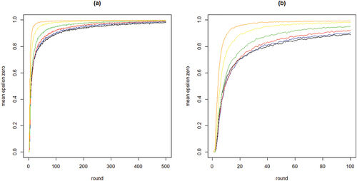
To further inspect properties (i) and (ii) Figure 2 plots the means per neighborhood size across the first 500 and the first 100 rounds. Figure 2 shows clearly how the mean curve of the ${\epsilon }_0\left(\mathit{n}\right)$ values consistently shifts upward as k increases: the more neighbors every agent learns from, the less informative any agent’s behavior is of their private experiences.

Figure 2. Mean proportions of agents staying with their object of choice given that it failed (${\epsilon }_0\left(\mathit{n}\right)$) on the y-axis by round on the x-axis; 100 runs for each neighborhood size k; black = 2 neighbors, blue = 4 neighbors, red = 8 neighbors, green = 16 neighbors, yellow = 32 neighbors, orange = 64 neighbors; agents learn optimally.

Looking at the first property of CA of theoretical interest, we find that the proportion of agents converging on a high-quality object is 1 or very close to 1 for all values of k. This is as it should be, since learning is “optimal” in that agents are informed of the true proportion of “false stayers” in the population, in each round. For neighborhood size 2, all 100 runs converge on all agents choosing a high-quality object. For neighborhood sizes 4 and 8, a single run converges on a situation where a single agent has not chosen a high-quality object (yet). For neighborhood sizes 16 and 64, two runs converge on a situation in which a single agent has not yet chosen a high-quality object. Neighborhood size 32 has five runs in which one or two agents do not yet converge on a high-quality object. Since Figure 1 reveals that ${\epsilon }_0\left(\mathit{n}\right)$ is consistently very close or equal to 1 for later rounds, these agents would eventually also move to a high-quality object if we allowed the models to run even longer (eventually, pure reinforcement learning will reveal object quality, given pH > pL). Thus, under optimal learning conditions “herding” (all agents converging on a low-quality object) does not, strictly speaking, occur (but see our discussion of search costs below).

The second property of CA of theoretical interest is the degree of inequality among high-quality objects, in terms of the number of agents choosing them, at convergence. Figure 3 shows the boxplots of the distributions of the Gini coefficients across the 100 runs per neighborhood size. A clear pattern unfolds: increasing k leads to rising inequality among high-quality objects. Thus, a central property of CA (inequality among equally good objects) emerges as agents socially learn from more neighbors, under optimal learning. When neighborhoods are small, optimal social learning is local and agents converge on distinct high-quality objects. When neighborhood size increases, however, CA emerges as a larger number of agents converge on the same high-quality object.

Figure 3. Boxplots of the distributions of Gini coefficients of the distribution of agent choices among high quality objects; Gini coefficients of 100 runs at convergence, per value of k.

Finally, we look at property (iii) of our model and the search costs for different values of k. Since virtually all runs show all agents converging on a high-quality object, Eq. (5)(5) $\mathit{s}\left(\mathit{n}\right)=1-\frac{\mathit{p}\left(\mathit{n}\right)-\mathit{pL}}{\mathit{pH}-\mathit{pL}}$(5) is a valid measure for the costs involved in collectively identifying a high-quality object. Figure 4 shows boxplots of the distributions of search costs (equation (5)(5) $\mathit{s}\left(\mathit{n}\right)=1-\frac{\mathit{p}\left(\mathit{n}\right)-\mathit{pL}}{\mathit{pH}-\mathit{pL}}$(5) summed over all rounds n, per run) for each value of k. Two properties are apparent: (i) search costs generally decline for increasing values of k, while (ii) some very high-cost runs emerge for higher values of k.

Figure 4. Boxplots of total search costs until convergence (based on Eq. (5) summed over all rounds n per run) for all values of k; y-axis running from 0 to 350 for k equal to 2, 4, and 8, from 0 to 8000 for k equal to 16 and 32, and from 0 to 20,000 for k equal to 64.

Wrapping up our analysis of optimal learning, we conclude that increasing the neighborhood size, k, leads to a steep increase of the extent of the “herd externality:” agents’ behaviors are less and less informative of their private experience. Since learning is optimal, there is no “herding;” rather, all agents converge on a high-quality object. The analysis of search costs, however, shows that, with higher values of k, some runs become excessively costly. Herding early on in the process can lead to extended periods in which many agents stick with a low-quality object (leading to very high values of Eq. (5)(5) $\mathit{s}\left(\mathit{n}\right)=1-\frac{\mathit{p}\left(\mathit{n}\right)-\mathit{pL}}{\mathit{pH}-\mathit{pL}}$(5) ). Such “temporary herding” does not occur with moderate and low values of k.

Finally, extreme inequality among equally good high-quality objects associated with CA appears as neighborhood size increases. Thus, based on a model of optimal learning, we can answer our second research question as follows: CA is a property of a mechanism in which agents learn rationally about object quality from their own experiences and from observing others. Additionally, a trade-off becomes apparent from the optimal learning analysis: reducing search costs by increasing neighborhood size leads to sharp increases in inequality, in addition to creating the risk of all agents getting stuck with a low-quality object for extended lengths of time.

5.2. Common knowledge of rationality

We now turn to the second part of our analyses, where agents lack the information on the true rate of “false stayers” and use a fixed value for ${\epsilon }_0$ throughout. We maintain the common knowledge assumption and fix ${\epsilon }_1$ at zero. In this “common knowledge of rationality” scenario we assume that all agents use the same unique value of ${\epsilon }_0$ for all rounds n, and explore values from 0 to 0.95 in steps of 0.05, adding 0.99 as an upper-bound. As ${\epsilon }_0$ gets closer to 1, agents put less and less prior probability on any neighbor leaving (${\epsilon }_0=1$ would imply zero prior probability of leaving, which would mean agents’ beliefs are not defined for cases in which a neighbor does leave). We run the model 20 times for each value of ${\epsilon }_0$.

Figure 5 shows the proportions of agents converging on a high-quality object as a function of ${\epsilon }_0$, for different values of k. Four properties of our model are apparent: (i) mean proportions increase in ${\epsilon }_0$ for all values of k, (ii) mean proportions for any given value of ${\epsilon }_0$ tend to increase with k, especially for low and moderate values of k (2 through 8), (iii) for values of ${\epsilon }_0$ below approximately 0.6, the dispersion in proportions increases with k, and (iv) for higher values of k (16, 32, and 64) this dispersion gives rise to increasing bifurcation in the sense that either all agents converge on a high-quality object or all agents converge on a low-quality object. Thus, increasing the mean proportion of agents finding a high-quality object by increasing neighborhood size k comes at the price of an increased risk of herding, i.e., all agents converging on a low-quality object.⁹

Figure 5. Proportions of agents converging on high quality (HQ) object for each value of ${\epsilon }_0$, for all values of k; 20 runs per value of ${\epsilon }_0$; solid lines depict mean proportions; dots are jittered for better representation.

Figure 6 shows the inequality among high-quality objects as measured by the Gini coefficient as a function of ${\epsilon }_0$, for all values of k. Note that these Gini coefficients are only defined when at least one agent converges on a high-quality object. Clearly, inequality among high-quality objects generally decreases in ${\epsilon }_0$. However, for moderate and high values of k (16, 32, and 64), inequality is consistently high up until (very) high values of ${\epsilon }_0$, only to decrease precipitously at the very end. Thus, larger neighborhood sizes k are associated with high degrees of inequality among (equally good) high-quality objects.

Figure 6. Gini coefficient values among high quality (HQ) objects in terms of numbers of agents choosing objects for each value of ${\epsilon }_0$, for all values of k; 20 runs per value of ${\epsilon }_0$; data for runs that have at least one agent converging on an HQ object; solid lines depict mean Gini.

Finally, Figures 7 plots the search costs measured as the sum of Eq. (5)(5) $\mathit{s}\left(\mathit{n}\right)=1-\frac{\mathit{p}\left(\mathit{n}\right)-\mathit{pL}}{\mathit{pH}-\mathit{pL}}$(5) across all rounds until convergence for only those runs in which all agents converge on a high-quality object (see Figure B1 in Appendix B for the search costs in all runs). Figures 7 reveals how search costs are generally increased when social learning is turned off and are lower for higher values of k.

Figure 7. Search costs according to Eq. (5) for different values of ${\epsilon }_0$, for each values of k; runs that end in all agents converging on a HQ object only.

These results paint the following picture. Across all neighborhood sizes, relying more on reinforcement learning than on social learning (i.e., increasing ${\epsilon }_0$) increases the mean proportion of agents ending up with a high-quality object, decreases inequality among such objects, and increases search costs. More importantly, however, increasing the neighborhood size k increases the mean proportion of agents finding a high-quality object, increases the probability that all agents end up with a high-quality object, but simultaneously increases the probability of herding. Moreover, when k increases, inequality among high-quality objects sharply increases as well. Therefore, in line with our results under optimal learning, CA with all its advantages (cheap collective convergence on high-quality objects) and disadvantages (non-trivial probability of herding and extreme unwarranted inequality among high-quality objects) emerges as the neighborhood size increases. Thus, again, CA emerges from a model of rationally learning agents looking for high-quality objects, provided agents practice some social learning and learn from a sufficiently large number of neighbors (our second research question).

5.3. Private knowledge of rationality

In this section, we drop the common knowledge of rationality assumption and assume that agents believe ${\epsilon }_1$ can be nonzero. We let $\mathit{\epsilon }={\epsilon }_0={\epsilon }_1$ and vary $\mathit{\epsilon }$ from 0 to 0.5 in steps of 0.05. Thus, $\mathit{\epsilon }$ represents the subjective probability that other agents act contrary to their experience. Note that $\mathit{\epsilon }=\frac{1}{2}$ implies that agents learn nothing from observing neighbors’ behaviors and all learning is reinforcement learning. The figures depicting outcomes from this scenario are in Appendix B. They are very similar to the corresponding figures from the common knowledge scenario. We focus on the qualitative patterns in the results in this section.

The mean proportions of agents converging on a high-quality object increase as $\mathit{\epsilon }$ gets closer to ½. Again, a bifurcation pattern emerges as k increases: larger neighborhood sizes imply an increased probability of all agents converging on a high-quality object but also an increased probability of herding.¹⁰

As before, increasing the neighborhood size k leads to dramatic increases in inequality among high-quality objects. Search costs decrease when k increases, regardless of whether convergence is on a high- or low-quality object. The analysis of our model under the private knowledge of rationality assumption reveals by now familiar pattern. Increasing the neighborhood size k leads to the emergence of CA with all its attendant consequences: a higher probability of cheap convergence on a high-quality object and an increased risk of herding, coupled with sharply increasing inequality among high-quality objects. Dropping the common knowledge of rationality assumption exacerbates the herding problem while simultaneously leading to lower probabilities of all agents finding a high-quality object, compared to the common knowledge of rationality scenario.

5.4. Answering our research questions

Considering all our analyses, we can answer our second research question. Generally, CA with all its advantages and drawbacks emerges as an unintended consequence of the behaviors of a population of agents attempting to select a high-quality object from a set containing a mix of high- and low-quality objects. The only prerequisite for CA to emerge is that agents practice at least some rational social learning and learn from a sufficiently large number of others. Whether or not their learning is “informed and optimal,” or whether or not the assumption of common knowledge of rationality holds, hardly affects the basic system-level patterns.

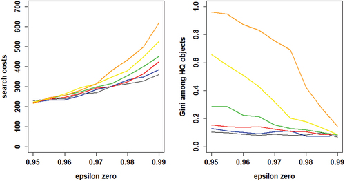
This leaves our first research question: can we get the advantages of CA without its disadvantages? Our analyses thus far suggest that we cannot. After all, all our results thus far point to the same basic trade-off: in order to decrease search costs, agents must learn from a larger number of others (i.e., k must increase). But increasing k inevitably leads to increased risks of herding and increased inequality. Yet if we take the analysis under the common knowledge assumption as our point of departure and zoom in on values of ${\epsilon }_0$ close to 1, this trade-off is actually flipped around. For values of ${\epsilon }_0$ near 1 all runs for all values of k show convergence of all agents on a high-quality object, but this is hardly surprising since agents then rely mainly on reinforcement learning. More importantly, as Figure 8 shows, in this range mean search costs (left panel) are actually lower for low values of k as are mean Gini values (right panel). Hence, as an illustration, we investigate the scenario under the common knowledge assumption with k = 2 and ${\epsilon }_0=0.95$ as a relatively promising situation in which the advantages of CA (relatively cheap collective convergence on a high-quality object) are present while the drawbacks (herding risk and excessive inequality among high-quality objects) are relatively mitigated. We run this scenario for 100 runs and compare to optimal learning in which agents are informed of the true rate of false stayers.

Figure 8. Average outcomes of learning under the common knowledge of rationality assumption; the left panel shows mean search costs, the right panel shows mean Gini coefficients. Neighborhood sizes: black for k = 2, blue for k = 4, red for k = 8, green for k = 16, yellow for k = 32, and orange for k = 64.

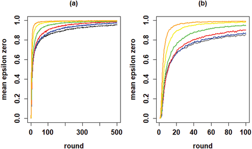
Figure 9 plots the development of the herd externality in this relatively promising scenario against that in the optimal learning scenario. The dotted line in the right-hand panel shows the constant value of 0.95 that agents use for ${\epsilon }_0$ in the common knowledge scenario. The temporal development of the herd externality in these plots looks very similar, but one result stands out. In the common knowledge scenario, convergence is much quicker due to the fact that agents rely more heavily on social learning after around 1,000 rounds. Further, since in both scenarios all agents converge on a high-quality object, this quicker convergence does not come at a price. In fact, comparing the distributions of the search costs in Figure B6 in Appendix B shows that in the common knowledge scenario the search cost distribution is, on average, slightly lower and more compressed. Moreover, Figure 7 shows the same for the distribution of Gini coefficients among the high-quality objects.

Figure 9. Proportions of agents staying with their object of choice given that it failed (${\epsilon }_0\left(\mathit{n}\right)$) on the y-axis by round on the x-axis; gray lines depict 100 runs, blue lines plot means per round; the optimal learning scenario is depicted in the left-hand plot and the “most promising” common knowledge scenario in the right-hand plot.

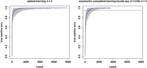
Thus, a scenario in which agents learn from just a few neighbors (k = 2 in our example) and rely relatively heavily on reinforcement learning (${\epsilon }_0=0.95$ in our example) does bring out the advantages of CA in the form of relatively cheap convergence of all agents on a high-quality object, while simultaneously having low levels of inequality among high-quality objects and no risk of herding. We can therefore answer our first research question with a qualified “yes.”

Intriguingly, this has unexpected implications for the social dynamics of CA processes. Think of the position of a single agent in the system. A look at the right-hand panel of Figure 9 reveals that for the first 1,000 rounds or so, an individual agent could rationally learn more from her neighbors than she is doing at ${\epsilon }_0=0.95$, as the herd externality is actually lower there. Beyond about 1,000 rounds, however, an individual agent should rationally learn less than she is doing at this value of ${\epsilon }_0$. But if each individual agent was to follow such an individually more rational social learning trajectory, the system would move toward optimal learning, which would slightly increase mean search costs and mean inequality and increase the spread of the distributions of these quantities (figures B6 and B7). What is more, regardless of what all other agents do, each agent individually has an incentive to learn from as many neighbors as possible. But if all agents do so the system ends up in a state like that in the lower right-hand plot of Figure 6, with extreme inequality among high-quality objects. Finally, all agents acting on both these individual incentives simultaneously puts us back in a situation akin to optimal learning with k = 64 with CA back in full force: on average cheap collective convergence on a high-quality object with a non-trivial risk of very expensive (temporary) herding, accompanied by extreme inequality among high-quality objects. It follows that CA has central features of a social dilemma: preventing its drawbacks is possible only if agents refrain from acting on “selfish” individual incentives to optimize their social learning.

6. Discussion

This paper shows how cumulative advantage arises from a micro-model of rational learning. Our model embeds agents in an environment in which they choose repeatedly and simultaneously, observing the choices of a subset of others. We investigate three degrees of rationality, ranging from an “optimal learning scenario” to a “private knowledge of rationality” scenario, along with an intermediate “common knowledge of rationality” scenario. Despite their differences, these three sets of analyses result in similar system-level outcomes: within each scenario increased reliance on reinforcement learning leads to a higher proportion of agents converging on a high-quality object, to higher search costs, and to less inequality among high-quality objects. Moreover, in each scenario increasing the neighborhood size k generally lowers search costs until convergence, but sharply increases inequality, and increases both the probability of collective convergence on a high-quality object and of herding (either temporary or permanent, depending on the scenario). Thus, we consistently observe a clear trade-off: efforts to decrease search costs by learning more from the behavior of more neighbors backfire, leading to runaway inequality and increased risks of herding (i.e., all agents converging on a low-quality object).

Given these results, we end our main analyses with an ancillary analysis of a relatively promising scenario in an effort to answer our first research question, namely whether societies can enjoy the upsides of cumulative advantage processes (all agents finding a high-quality object at low search costs) without suffering the downsides (heightened inequality and increased risk of herding). We answer this question with a qualified yes. Additionally, the ancillary analysis shows that CA processes have features of a social dilemma: agents acting on individual incentives create suboptimal collective outcomes.

6.1. Directions for Future Research

The current paper uses random regular graphs to link agents to neighbors. This effectively implies agents in our model are coupled with a random sample from the population. This means that, allowing for sampling bias, individual agents “on average” learn what the entire population learns. An interesting avenue for future research is the exploration of the effects of network topology on our results. For instance, various degrees of local clustering in regular graphs would create networks with more or less small world properties. This would open up the possibility of more “localized learning dynamics” where what agents learn in their local “community” can very quickly diverge from what others learn in theirs. One important question for future research is the extent to which such local clustering could prevent the drawbacks of CA without dissipating its advantages. Other network hypotheses could also be generated and our current model has laid the groundwork for this.

Other possible directions for future work include experimental tests of the current model and of its applications to various network structures. Experimental treatments could vary the neighborhood sizes of participants and could manipulate the extent to which they discount the behavior of others, for instance by stressing (or not) that their neighbors are also socially learning from others. A particularly interesting experimental study using these manipulations would be to compare the extent of CA and herding on random regular graphs and on small world graphs with the same degree, along the lines of work by Centola (2011) on diffusion dynamics.

Disclosure statement

No potential conflict of interest was reported by the author(s).

Notes

¹ In the behavioral game theory literature (Camerer, 2003) this mode of learning would be called “belief learning.” However, since all our learning is rational and thus based on beliefs, we opt for the term “reinforcement learning.” This conveys the information that this form of learning is based on an agent’s own experience. Just like with non-rational forms of reinforcement learning (cf. Flache & Macy, 2002) our rational reinforcement learning implies that the experience of success makes a repeated choice of the same object more likely, whereas failure makes it less likely.

² For these beliefs to be truly well-defined after all histories, it is required that “zero-probability events” do not occur. In particular, when appropriate we will be assuming that ${\epsilon }_0<1$, since ${\epsilon }_1=0$ and ${\epsilon }_0=1$ together imply that neighbor j always stays (rendering “leave” a zero-probability event).

³ When values of ½ are plugged in for both epsilons in Eqs. (4)(4) $P_i\left(H_{o^{\prime }}|\mathit{leave}\left(\mathit{j},\mathit{o}{ }^{\mathrm{\prime }}\right)\right)=\frac{\left[\left(1-{\epsilon }_0\right)\left(1-p_H\right)+{\epsilon }_1{p}_H\right]P_i\left(H_{o^{\prime }}\right)}{\left[\left(1-{\epsilon }_0\right)\left(1-p_H\right)+{\epsilon }_1{p}_H\right]P_i\left(H_{o^{\prime }}\right)+\left[\left(1-{\epsilon }_0\right)\left(1-p_L\right)+{\epsilon }_1{p}_L\right]\left(1-P_i\left(H_{o^{\prime }}\right)\right)}$(4) and (5(5) $\mathit{s}\left(\mathit{n}\right)=1-\frac{\mathit{p}\left(\mathit{n}\right)-\mathit{pL}}{\mathit{pH}-\mathit{pL}}$(5) ) the posteriors equal the priors.

⁴ This operationalization of “optimal learning” resembles a procedure used by Anderson and Holt (1997). These authors conduct an experimental investigation of the model of Bikhchandani et al. (1992), and in their ex post (i.e., after having observed participants’ behavior) determination of optimal choice behavior they estimate error rates (i.e. deviations from Bayesian optimality) for each round and use those estimates to determine optimal behavior in the next. The key difference with our current approach, apart from the fact that our agents are of course simulated, is that our “false stayers” do not deviate from Bayesian optimality, whereas Anderson & Holt’s participants do.

⁵ Note that the latter does not imply that the difference in consequences of success or failure is unimportant. We do not model the value to the agents of success or failure, but simply assume ordinal preferences in this respect: agents like success better than failure.

⁶ For each model run separately, we generated a random regular graph with the specified neighborhood size using the function sample_k_regular from the igraph package (Csardi & Nepusz, 2006). The support of this function consists of the space of connected k-regular graphs in which there exists at most one edge between any pair of nodes (i.e., no multigraphs). Thus, each connected regular k-graph of specified neighborhood size has a strictly positive probability of being drawn. The function does not guarantee a uniform draw (equiprobability of all connected regular k-graphs), however. To guarantee uniformity, we would have to employ the function sample_degseq, but this would come at the price of increasing the runtime of our models. Considering the relatively large number of runs we need for our paper (including robustness checks) we opted for using sample_k_regular directly. We believe the lack of uniformity in no way affects our conclusions, because nodes have no properties beyond their labels. In addition, since beliefs about object quality are uniform at the outset, object choice in the first round is entirely random.

⁷ Note that the model does not harbor any “repeated game strategic incentives:” each agent simply wants to maximize the probability of choosing a high quality object in each round, and hence has an incentive to learn optimally from the behavior of her neighbors in each round separately.

⁸ Note that the “false stayer rate” is not information agents would normally have in real-world applications. We included this treatment to investigate a situation with “complete information” that allows agents to “optimally adjust their aim” after each round. Initially, we wanted to use the approach in this treatment to locate a Nash equilibrium of the system (from the potentially very large set of equilibria). To do so, we took the following approach. We ran our current optimal learning model in a series of subsequent “sessions” (each comprised of 20 runs), each time feeding the agents in a new session the average learning trajectory (i.e., the profile of average false stayer rates in each round, across the runs) of the previous session. While for neighborhood sizes 2 and 4 this eventually yielded a stable learning trajectory (which would thus be a “fixed point” of the system and hence a Nash equilibrium), this procedure failed to converge for larger neighborhoods. We have therefore chosen to postpone the issue of computationally finding Nash equilibria to future research, and include the current optimal learning treatment as an investigation of what optimal behavior would look like if agents had access to the (informationally aggregated) learning histories of their peers.

⁹ Across all values of ${\epsilon }_0$, the percentages of runs ending in such herding are 0 for k equal to 2, 4, and 8, but 2.62%, 7.14%, and 12.38% for k equal to 16, 32, and 64, respectively. The percentages of runs ending in all agents converging on a high quality object are 16.67%, 20.71%, 43.10%, 81.67%, 88.57%, and 85.48% for k equal to 2, 4, 8, 16, 32, and 64, respectively.

¹⁰ Leaving out the trivial case of $\mathit{\epsilon }=\frac{1}{2}$, the probabilities of herding are 0 for k equal to 2, 4, and 8, and 0.12, 0.26, and 0.39 for k equal to 16, 32, and 64, respectively. The probabilities of all agents converging on a high-quality object for the same sequence of k are 0, 0, 0.12, 0.59, 0.68, and 0.59, respectively.

Appendix A.

Deriving equations (3) and (4)

In this appendix, let y be the observed behavior of a neighbor, with $\mathit{y}=\left\{\begin{array}{c}0,\mathit{if}\mathit{neighbor}\mathit{leaves}\\ 1,\mathit{if}\mathit{neighbor}\mathit{stays}\end{array}\right.$.

P(H) and P(H|y) denote the prior and posterior probabilities of the object being high quality. Let P(success|H) = p_H and P(success|L) = p_L be the success probabilities of high and low-quality types, respectively. As in the paper, P(y = 0|success) = ε₁ and P(y = 1|failure) = ε₀.

First consider P(H|y = 1). Bayes’ Rule gives $\mathit{P}\left(\mathit{H}|\mathit{y}=1\right)=\frac{\mathit{P}\left(\mathit{y}=1|H\right)P\left(H\right)}{\mathit{P}\left(\mathit{y}=1\right)}$. Analyzing this formula term by term, we get:

$\mathit{P}\left(\mathit{y}=1|\mathit{H}\right)=\mathit{P}\left(\mathit{y}=1,\mathit{failure}|\mathit{H}\right)+\mathit{P}\left(\mathit{y}=1,\mathit{success}|\mathit{H}\right)$

$=\mathit{P}\left(\mathit{y}=1|\mathit{failure}\right)\mathit{P}\left(\mathit{failure}|\mathit{H}\right)+\mathit{P}\left(\mathit{y}=1|\mathit{success}\right)\mathit{P}\left(\mathit{success}|\mathit{H}\right)$

(A1) $={\epsilon }_0\left(1-p_H\right)+\left(1-{\epsilon }_1\right)p_H$(A1)

Similarly, $\mathit{P}\left(\mathit{y}=1|\mathit{L}\right)={\epsilon }_0\left(1-p_L\right)+\left(1-{\epsilon }_1\right)p_L$, and combining with (A1) yields:

(A2) $\mathit{P}\left(\mathit{y}=1\right)=\left[{\epsilon }_0\left(1-p_H\right)+\left(1-{\epsilon }_1\right)p_H\right]\mathit{P}\left(\mathit{H}\right)+\left[{\epsilon }_0\left(1-p_L\right)+\left(1-{\epsilon }_1\right)p_L\right]\left(1-\mathit{P}\left(\mathit{H}\right)\right)$(A2)

Using Bayes’ Rule with (A1) and A2) yields:

$\mathit{P}\left(\mathit{H}|\mathit{y}=1\right)=\frac{\left[{\epsilon }_0\left(1-p_H\right)+\left(1-{\epsilon }_1\right)p_H\right]\mathit{P}\left(\mathit{H}\right)}{\left[{\epsilon }_0\left(1-p_H\right)+\left(1-{\epsilon }_1\right)p_H\right]\mathit{P}\left(\mathit{H}\right)+\left[{\epsilon }_0\left(1-p_L\right)+\left(1-{\epsilon }_1\right)p_L\right]\left(1-\mathit{P}\left(\mathit{H}\right)\right)}$, which is Equation A2(A2) $\mathit{P}\left(\mathit{y}=1\right)=\left[{\epsilon }_0\left(1-p_H\right)+\left(1-{\epsilon }_1\right)p_H\right]\mathit{P}\left(\mathit{H}\right)+\left[{\epsilon }_0\left(1-p_L\right)+\left(1-{\epsilon }_1\right)p_L\right]\left(1-\mathit{P}\left(\mathit{H}\right)\right)$(A2) form the paper.

Using the same steps we get, mutatis mutandis:

$\mathit{P}\left(\mathit{H}|\mathit{y}=0\right)=\frac{\left[\left(1-{\epsilon }_0\right)\left(1-p_H\right)+{\epsilon }_1{p}_H\right]\mathit{P}\left(\mathit{H}\right)}{\left[\left(1-{\epsilon }_0\right)\left(1-p_H\right)+{\epsilon }_1{p}_H\right]\mathit{P}\left(\mathit{H}\right)+\left[\left(1-{\epsilon }_0\right)\left(1-p_L\right)+{\epsilon }_1{p}_L\right]\left(1-\mathit{P}\left(\mathit{H}\right)\right)}$, which is equation (4)(4) $P_i\left(H_{o^{\prime }}|\mathit{leave}\left(\mathit{j},\mathit{o}{ }^{\mathrm{\prime }}\right)\right)=\frac{\left[\left(1-{\epsilon }_0\right)\left(1-p_H\right)+{\epsilon }_1{p}_H\right]P_i\left(H_{o^{\prime }}\right)}{\left[\left(1-{\epsilon }_0\right)\left(1-p_H\right)+{\epsilon }_1{p}_H\right]P_i\left(H_{o^{\prime }}\right)+\left[\left(1-{\epsilon }_0\right)\left(1-p_L\right)+{\epsilon }_1{p}_L\right]\left(1-P_i\left(H_{o^{\prime }}\right)\right)}$(4) from the paper.

Appendix B.

Supplemental figures

Supplemental figure for the common knowledge of rationality scenario

Figure B1. Search costs according to Eq. (5) for different values of ${\epsilon }_0$, for each values of k; all runs.

Figures for the private knowledge of rationality scenario

Figure B2. Proportions of agents choosing a HQ object at convergence for different values of $\mathit{\epsilon }$, for each value of neighborhood size k; solid lines are mean proportions.

Figure B3. Gini coefficient values among HQ objects for different values of $\mathit{\epsilon }$, for all values of k.

Figure B4. Search costs according to Eq. (5)(5) $\mathit{s}\left(\mathit{n}\right)=1-\frac{\mathit{p}\left(\mathit{n}\right)-\mathit{pL}}{\mathit{pH}-\mathit{pL}}$(5) for different values of $\mathit{\epsilon }$ across all runs for each value of k.

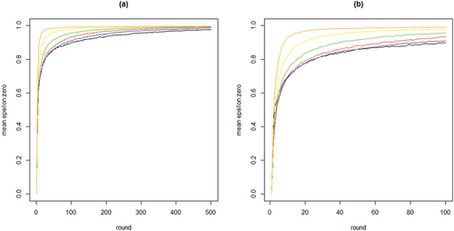
Figure B5. Search costs according to Eq. (5)(5) $\mathit{s}\left(\mathit{n}\right)=1-\frac{\mathit{p}\left(\mathit{n}\right)-\mathit{pL}}{\mathit{pH}-\mathit{pL}}$(5) for different values of $\mathit{\epsilon }$ for runs ending in all agents converging on a high-quality object only, for all values of k.

Supplemental figures for the comparison of optimal learning and the “most promising scenario”

Figure B6. Box-plots of search costs in the optimal learning condition (left-hand) and the “most promising” common knowledge condition; neighborhood size k equals 2.

Figure B7. Boxplots if Gini coefficients at convergence in the optimal learning condition (left-hand) and the “most promising” common knowledge condition; neighborhood size k equals 2.

Appendix C.

Robustness Checks

In this appendix, we check the robustness of the “optimal learning” model results reported in the paper for two different values of the h parameter and three different values of the parameter vector $\left(p_L,p_H\right)$. We focus on optimal learning, because all the basic aspects of the pattern were borne out in this scenario, including the “temporary herding” of agents on low-quality objects. The optimal learning scenario thus reflected all theoretically interesting phenomena we set out to investigate in this paper, and we are curious to what extend changes in parameter settings affect these basic patterns in understandable ways.

Changes in h affect the initial prior belief h/O. Since CA is inherently a process that is sensitive to initial conditions, we investigate h = 5 (as in the paper, for a prior belief of 0.25) and h = 10 (for a prior of 0.5). The parameter vector $\left(p_L,p_H\right)$ affects learning in two ways. Absolute success rates of objects affect the total “noise” in the system, while relative success rates affect the degree to which agents can experientially discriminate between high- and low-quality objects given a level of overall noise. Hence, we manipulate absolute probabilities and odds ratios ($\mathit{OR}=\frac{p_H}{1-p_H}/\frac{p_L}{1-p_L}$) independently. This leads to the overview of robustness checks (RC) in Table C1. In all RCs, we retain the values of I = 200 and O = 40 from the paper, because the fact that I is much larger than O is a central feature of the social situations we model.

In each RC, we run our model in the optimal learning scenario. Below, we present the same figures for this scenario that we presented in the paper. These figures reveal the following pattern:

1. In RC0, RC1a, and RC1b, that have low odds ratios (i.e., small relative differences in success probabilities; $\mathit{OR}=\frac{4}{3}$) we observe the same basic pattern as in the model from the paper. There is a three-way trade-off between inequality, search costs, and herding risk: increasing neighborhood size k lowers average search costs, but engenders extreme inequality among high-quality objects and entails an increased risk of “temporary herding.” Notwithstanding these general patterns, low absolute success probabilities (RC1a) seem to increase the variance in inequality and search costs from run to run. Also, the high prior (h = 10) in RC1b and RC0 appears to mitigate the herding risk. These facts are unsurprising, as success probabilities closer to ½ increase the noise in the system and more abundant types of objects are easier to find.

2. The much higher relative difference in success probability in RC2 and RC3 ($\mathit{OR}=\frac{8}{3})$ turns the three-way trade-off into a two-way trade-off. Increasing neighborhood size k still lowers search costs and sharply increases inequality. However, due to the high difference in success probability between low- and high-quality objects, the risk of temporary herding is now gone. This is again unsurprising, since high odds ratios make reinforcement learning much more potent and thus decrease the risk of any agent sticking with a low-quality object for long periods of time.

Overall, the conclusion from the RCs in the optimal learning scenario is that CA, with its attendant advantage (low average search costs) and drawbacks (extreme inequality and risk of herding), is typical of situations with small differences in success probabilities between high- and low-quality objects and relatively scarce high-quality objects. But these are precisely the situations in which reinforcement learning is less effective and agents will want to rely on social learning. Thus, social learning is most dangerous when it is most potent.

Table C1. Parameter values for robustness checks.

Robustness Check (RC)	Value of h	Value of $\left(p_L,p_H\right)$	OR
Model from paper	5	$\left(\frac{3}{4},\frac{4}{5}\right)$	$\frac{4}{3}$
RC0	10	$\left(\frac{3}{4},\frac{4}{5}\right)$	$\frac{4}{3}$
RC1a	5	$\left(\frac{1}{3},\frac{2}{5}\right)$	$\frac{4}{3}$
RC1b	10	$\left(\frac{1}{3},\frac{2}{5}\right)$	$\frac{4}{3}$
RC2a	5	$\left(\frac{3}{5},\frac{4}{5}\right)$	$\frac{8}{3}$
RC2b	10	$\left(\frac{3}{5},\frac{4}{5}\right)$	$\frac{8}{3}$
RC3a	5	$\left(\frac{1}{5},\frac{2}{5}\right)$	$\frac{8}{3}$
RC3b	10	$\left(\frac{1}{5},\frac{2}{5}\right)$	$\frac{8}{3}$

1. RC0

Figure C.1.1. Proportions of agents staying with their object of choice given that it failed (${\epsilon }_0\left(\mathit{n}\right)$) on the y-axis by round on the x-axis; gray lines depict 100 runs for each neighborhood size k, black lines plot means per round; agents learn optimally; RC0.

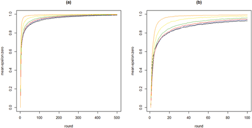
Figure C.1.2. Mean proportions of agents staying with their object of choice given that it failed (${\epsilon }_0\left(\mathit{n}\right)$) on the y-axis by round on the x-axis; 100 runs for each neighborhood size k; black = 2 neighbors, blue = 4 neighbors, red = 8 neighbors, green = 16 neighbors, yellow = 32 neighbors, orange = 64 neighbors; agents learn optimally; RC0.

Figure C.1.3. Boxplots of the distributions of Gini coefficients of the distribution of agent choices among high quality objects; Gini coefficients of 100 runs at convergence, per value of k; agents learn optimally; RC0.

Figure C.1.4. Boxplots of total search costs until convergence (based on equation (5) summed over all rounds n per run) for all values of k; y-axis running from 0 to 350 for k equal to 2, 4, and 8, from 0 to 8000 for k equal to 16 and 32, and from 0 to 20,000 for k equal to 64; agents learn optimally; RC0.

2. RC1a

Figure C.2.1. Proportions of agents staying with their object of choice given that it failed (${\epsilon }_0\left(\mathit{n}\right)$) on the y-axis by round on the x-axis; gray lines depict 100 runs for each neighborhood size k, black lines plot means per round; agents learn optimally; RC1a.

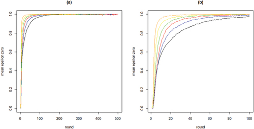
Figure C.2.2. Mean proportions of agents staying with their object of choice given that it failed (${\epsilon }_0\left(\mathit{n}\right)$) on the y-axis by round on the x-axis; 100 runs for each neighborhood size k; black = 2 neighbors, blue = 4 neighbors, red = 8 neighbors, green = 16 neighbors, yellow = 32 neighbors, orange = 64 neighbors; agents learn optimally; RC1a.

Figure C.2.3. Boxplots of the distributions of Gini coefficients of the distribution of agent choices among high quality objects; Gini coefficients of 100 runs at convergence, per value of k; agents learn optimally; RC1a.

Figure C.2.4. Boxplots of total search costs until convergence (based on Eq. (5)(5) $\mathit{s}\left(\mathit{n}\right)=1-\frac{\mathit{p}\left(\mathit{n}\right)-\mathit{pL}}{\mathit{pH}-\mathit{pL}}$(5) summed over all rounds n per run) for all values of k; y-axis running from 0 to 350 for k equal to 2, 4, and 8, from 0 to 8000 for k equal to 16 and 32, and from 0 to 20,000 for k equal to 64; agents learn optimally; RC1a.

3. RC1b

Figure C.3.1. Proportions of agents staying with their object of choice given that it failed (${\epsilon }_0\left(\mathit{n}\right)$) on the y-axis by round on the x-axis; gray lines depict 100 runs for each neighborhood size k, black lines plot means per round; agents learn optimally; RC1b.

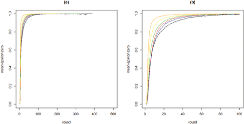
Figure C.3.2. Mean proportions of agents staying with their object of choice given that it failed (${\epsilon }_0\left(\mathit{n}\right)$) on the y-axis by round on the x-axis; 100 runs for each neighborhood size k; black = 2 neighbors, blue = 4 neighbors, red = 8 neighbors, green = 16 neighbors, yellow = 32 neighbors, orange = 64 neighbors; agents learn optimally; RC1b.

Figure C.3.3. Boxplots of the distributions of Gini coefficients of the distribution of agent choices among high quality objects; Gini coefficients of 100 runs at convergence, per value of k; agents learn optimally; RC1b.

Figure C.3.4. Boxplots of total search costs until convergence (based on Eq. (5)(5) $\mathit{s}\left(\mathit{n}\right)=1-\frac{\mathit{p}\left(\mathit{n}\right)-\mathit{pL}}{\mathit{pH}-\mathit{pL}}$(5) summed over all rounds n per run) for all values of k; y-axis running from 0 to 350 for k equal to 2, 4, and 8, from 0 to 8000 for k equal to 16 and 32, and from 0 to 20,000 for k equal to 64; agents learn optimally; RC1b.

Figure C.4.1. Proportions of agents staying with their object of choice given that it failed ()on the y-axis by round on the x-axis; gray lines depict 100 runs for each neighborhood size k, black lines plot means per round; agents learn optimally; RC2a.

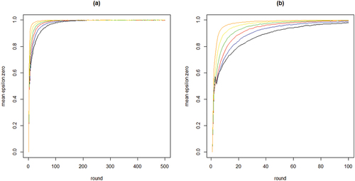
4. RC2a

Figure C.4.2. Mean proportions of agents staying with their object of choice given that it failed (${\epsilon }_0\left(\mathit{n}\right)$) on the y-axis by round on the x-axis; 100 runs for each neighborhood size k; black = 2 neighbors, blue = 4 neighbors, red = 8 neighbors, green = 16 neighbors, yellow = 32 neighbors, orange = 64 neighbors; agents learn optimally; RC2a.

Figure C.4.3. Boxplots of the distributions of Gini coefficients of the distribution of agent choices among high quality objects; Gini coefficients of 100 runs at convergence, per value of k; agents learn optimally; RC2a.

Figure C.4.4. Boxplots of total search costs until convergence (based on Eq. (5)(5) $\mathit{s}\left(\mathit{n}\right)=1-\frac{\mathit{p}\left(\mathit{n}\right)-\mathit{pL}}{\mathit{pH}-\mathit{pL}}$(5) summed over all rounds n per run) for all values of k; y-axis running from 0 to 350 for k equal to 2, 4, and 8, from 0 to 8000 for k equal to 16 and 32, and from 0 to 20,000 for k equal to 64; agents learn optimally; RC2a.

5. RC2b

Figure C.5.1. Proportions of agents staying with their object of choice given that it failed (${\epsilon }_0\left(\mathit{n}\right)$) on the y-axis by round on the x-axis; gray lines depict 100 runs for each neighborhood size k, black lines plot means per round; agents learn optimally; RC2b.

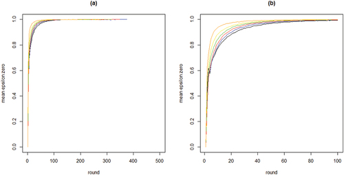
Figure C.5.2. Mean proportions of agents staying with their object of choice given that it failed (${\epsilon }_0\left(\mathit{n}\right)$) on the y-axis by round on the x-axis; 100 runs for each neighborhood size k; black = 2 neighbors, blue = 4 neighbors, red = 8 neighbors, green = 16 neighbors, yellow = 32 neighbors, orange = 64 neighbors; agents learn optimally; RC2b.

Figure C.5.3. Boxplots of the distributions of Gini coefficients of the distribution of agent choices among high quality objects; Gini coefficients of 100 runs at convergence, per value of k; agents learn optimally; RC2b.

Figure C.5.4. Boxplots of total search costs until convergence (based on Eq. (5)(5) $\mathit{s}\left(\mathit{n}\right)=1-\frac{\mathit{p}\left(\mathit{n}\right)-\mathit{pL}}{\mathit{pH}-\mathit{pL}}$(5) summed over all rounds n per run) for all values of k; y-axis running from 0 to 350 for k equal to 2, 4, and 8, from 0 to 8000 for k equal to 16 and 32, and from 0 to 20,000 for k equal to 64; agents learn optimally; RC2b.

6. RC3a

Figure C.6.1. Proportions of agents staying with their object of choice given that it failed (${\epsilon }_0\left(\mathit{n}\right)$) on the y-axis by round on the x-axis; gray lines depict 100 runs for each neighborhood size k, black lines plot means per round; agents learn optimally; RC3a.

Figure C.6.2. Mean proportions of agents staying with their object of choice given that it failed (${\epsilon }_0\left(\mathit{n}\right)$) on the y-axis by round on the x-axis; 100 runs for each neighborhood size k; black = 2 neighbors, blue = 4 neighbors, red = 8 neighbors, green = 16 neighbors, yellow = 32 neighbors, orange = 64 neighbors; agents learn optimally; RC3a.

Figure C.6.3. Boxplots of the distributions of Gini coefficients of the distribution of agent choices among high quality objects; Gini coefficients of 100 runs at convergence, per value of k; agents learn optimally; RC3a.

Figure C.6.4. Boxplots of total search costs until convergence (based on Eq. (5)(5) $\mathit{s}\left(\mathit{n}\right)=1-\frac{\mathit{p}\left(\mathit{n}\right)-\mathit{pL}}{\mathit{pH}-\mathit{pL}}$(5) summed over all rounds n per run) for all values of k; y-axis running from 0 to 350 for k equal to 2, 4, and 8, from 0 to 8000 for k equal to 16 and 32, and from 0 to 20,000 for k equal to 64; agents learn optimally; RC3a.

7. RC3b

Figure C.7.1. Proportions of agents staying with their object of choice given that it failed (${\epsilon }_0\left(\mathit{n}\right)$) on the y-axis by round on the x-axis; gray lines depict 100 runs for each neighborhood size k, black lines plot means per round; agents learn optimally; RC3b.

Figure C.7.2. Mean proportions of agents staying with their object of choice given that it failed (${\epsilon }_0\left(\mathit{n}\right)$) on the y-axis by round on the x-axis; 100 runs for each neighborhood size k; black = 2 neighbors, blue = 4 neighbors, red = 8 neighbors, green = 16 neighbors, yellow = 32 neighbors, orange = 64 neighbors; agents learn optimally; RC3b.

Figure C.7.3. Boxplots of the distributions of Gini coefficients of the distribution of agent choices among high quality objects; Gini coefficients of 100 runs at convergence, per value of k; agents learn optimally; RC3b.

Figure C.7.4. Boxplots of total search costs until convergence (based on Eq. (5)(5) $\mathit{s}\left(\mathit{n}\right)=1-\frac{\mathit{p}\left(\mathit{n}\right)-\mathit{pL}}{\mathit{pH}-\mathit{pL}}$(5) summed over all rounds n per run) for all values of k; y-axis running from 0 to 350 for k equal to 2, 4, and 8, from 0 to 8000 for k equal to 16 and 32, and from 0 to 20,000 for k equal to 64; agents learn optimally; RC3b.

References

- Anderson, L. R., & Holt, A. H. (1997). Information cascades in the laboratory. The American Economic Review, 87(5), 847–862. https://www.jstor.org/stable/2951328
- Banerjee, A. V. (1992). A simple model of herd behavior. Quarterly Journal of Economics, 107(3), 797–817. https://doi.org/10.2307/2118364
- Berger, S., Feldhaus, C., & Ochenfels, A. (2018). A shared identity promotes herding in an information cascade game. Journal of the Economic Science Association, 4(1), 63–72. https://doi.org/10.1007/s40881-018-0050-9
- Bicchieri, C. (2005). The grammar of society: The nature and dynamics of social norms. Cambridge University Press.
- Bikhchandani, S., Hirshleifer, D., & Welch, I. (1992). A theory of fads, fashion, custom, and cultural change as information cascades. Journal of Political Economy, 100(5), 992–1026. https://www.jstor.org/stable/2138632
- Bol, T., de Vaan, M., & van de Rijt, A. (2018). The Matthew effect in science funding. PNAS, 115(19), 4887–4890. https://doi.org/10.1073/pnas.17195571
- Camerer, C. F. (2003). Behavioral game theory: Experiments in strategic interaction. Princeton University Press & Russell Sage Foundation.
- Camerer, C. F., Ho, T. H., & Chong, J. K. (2004). A cognitive hierarchy model of games. Quarterly Journal of Economics, 119(3), 861–898. https://doi.org/10.1162/0033553041502225
- Centola, D. (2011). An experimental study of homophily in the adoption of health behavior. Science, 334, 1269–1272. https://doi.org/10.1126/science.1207055
- Centola, D. (2021). Change: How to make big things happen. Little, Brown Spark.
- Centola, D., Willer, R., & Macy, M. (2005). The Emperor’s Dilemma: A Computational Model of Self-Enforcing Norms. The American Journal of Sociology, 110(4), 1009–1040. https://doi.org/10.1086/427321
- Coleman, J. S. (1990). Foundations of social theory. Belknap Press of Harvard University Press.
- Csardi, G., & Nepusz, T. (2006). The igraph software package for complex network research. Inter Journal, Complex Systems, 1695. https://igraph.org
- DiMaggio, P., & Garip, F. (2012). Network effects and social inequality. Annual Review of Sociology, 38, 93–118. https://doi.org/10.1146/annurev.soc.012809.102545
- DiPrete, T. A., & Eirich, G. M. (2006). Cumulative advantage as a mechanism for inequality: A review of theoretical and empirical developments. Annual Review of Sociology, 32, 271–297. https://doi.org/10.1146/annurev.soc.32.061604.123127
- Easly, D., & Kleinberg, J. (2010). Networks, crowds, and markets: Reasoning about a highly connected world. Cambridge University Press.
- Flache, A., & Macy, M. W. (2002). Stochastic collusion and the power law of learning: A general reinforcement learning model of cooperation. The Journal of Conflict Resolution, 46(5), 629–653. https://doi.org/10.1177/002200202236167
- Frank, R. H., & Cook, P. J. (1995). The winner-take-all society: How more and more Americans compete for ever fewer and bigger prizes, encouraging economic waste, income inequality, and an impoverished cultural life. Free Press.
- Frey, V., & van de Rijt, A. (2016). Arbitrary inequality in reputation systems. Scientific Reports, 6, 38304. https://doi.org/10.1038/srep38304
- Gladwell, M. (2008). Outliers: The story of success. Little, Brown and Co.
- Haidt, J. (2012). The righteous mind: Why good people are divided by politics and religion. Pantheon Books.
- Hechter, M., & Kanazawa, S. (1997). Sociological rational choice theory. Annual Review of Sociology, 23, 191–214. https://www.jstor.org/stable/2952549
- Hedström, P. (2009). Dissecting the social. Cambridge University Press.
- Malle, B. F. (2006). The actor-observer asymmetry in attribution: A (surprising) meta-analysis. Psychological Bulletin, 132(6), 895–919. https://doi.org/10.1037/0033-2909.132.6.895
- Merton, R. K. (1968). The Matthew effect in science. Science, 159(3810), 56–63. https://doi.org/10.1126/science.159.3810.56
- Miller, D. T., & McFarland, C. (1987). Pluralistic ignorance: When similarity is interpreted as dissimilarity. Journal of Personality & Social Psychology, 53(2), 298–305. https://doi.org/10.1037/0022-3514.53.2.298
- Opp, K. D. (2009). Theories of political protest and social movements: A multidisciplinary introduction, critique, and synthesis. Routledge.
- Raafat, R. M., Chater, N., & Firth, C. (2009). Herding in humans. Trends in Cognitive Sciences, 13(10), 420–428. https://doi.org/10.1016/j.tics.2009.08.002
- R Core Team. (2017). R: A language and environment for statistical computing. R Foundation for Statistical Computing.
- Rosen, S. (1981). The economics of superstars. The American Economic Review, 71(5), 845–858. https://www.jstor.org/stable/1803469
- Ross, L. (1977). The intuitive psychologist and his shortcomings: Distortions in the attribution process. Advances in Experimental Social Psychology, 10, 173–220. https://doi.org/10.1016/S0065-2601(08)60357-3
- Salganik, M. J., Dodds, P. S., & Watts, D. J. (2006). Experimental study of inequality and unpredictability in an artificial cultural market. Science, 311, 854–856. https://doi.org/10.1126/science.1121066
- Simpson, B., & Aksoy, O. (2017). Cumulative advantage in collective action groups: How competition for group members alters the provision of public goods. Social Science Research, 66, 1–21. https://doi.org/10.1016/j.ssresearch.2017.03.001
- Stigler, G. J. (1961). The economics of information. Journal of Political Economy, 69(3), 213–225. https://www.jstor.org/stable/1829263
- Strang, D., & Macy, M. W. (2001). In search of excellence: Fads, success stories, and adaptive emulation. The American Journal of Sociology, 107(1), 147–182. https://doi.org/10.1086/323039
- Trueman, B. (1994). Analyst forecasts and herding behavior. The Review of Financial Studies, 7(1), 97–124. https://www.jstor.org/stable/2962287
- Watts, D. J. (2007). Is Justin Timberlake a product of cumulative advantage? New York Times, April 15. https://www.nytimes.com/2007/04/15/magazine/15wwlnidealab.t.html