Dynamical systems of self-organized segregation

ABSTRACT

We re-consider Schelling’s (1971) bounded neighborhood model as put into the form of a dynamical system by Haw and Hogan (2018). The aim is to determine how tolerance can prevent (or lead to) segregation. In the case of a single neighborhood, we explain the occurring bifurcation set, thereby correcting a scaling error. In the case of two neighborhoods, we correct a major error and derive a dynamical system that does satisfy the modeling assumptions made by Haw and Hogan (2020), staying as close as possible to their construction. We find that stable integration is then only possible if the populations in the two neighborhoods have the option to be in neither neighborhood. In the absence of direct movement between the neighborhoods, the problem is furthermore equivalent to independent single neighborhood problems.

KEYWORDS:

• Bounded neighborhood model
• structural stability
• unorganized segregation

1. Introduction

Segregation is a phenomenon in which people are separated based on factors such as ethnicity, religion or political preferences. It can manifest in a number of domains of everyday life, like residential districts, schools or workplaces, to name a few. In this paper, we focus on residential segregation in a district of a city. The broad mathematical definition of segregation that we use and the principles governing it, however, can be applied to a multitude of seemingly disparate situations, reaching as far as the division of members within a political party.

While residential segregation may be perceived by many as a phenomenon of the past, segregation still exists today in the twenty-first century. In some locations, patterns of segregation remain similar to the patterns of segregation of the past. For instance, the South African city of Chatsworth was created to segregate Indians during the Apartheid and even now, in the twenty-first century, Indians continue to make up the majority of Chatsworth’s population (Jones, 2019). In the USA, from 1980 to 2000, white and black segregation declined while Asian and Pacific Islander segregation increased (Iceland, 2004).

Segregation has several adverse effects on specific populations for both individuals and groups. Multiple studies (De la Roca et al., 2014, Williams and Collins, 2001, Cutler & Glaeser, 1997, Lewis, 1966) have provided empirical evidence that segregation, combined with poverty, leads to a multitude of problems. These problems include the reduction of contact of individuals with positive role models, increased exposure to violence, the promotion of a “culture of poverty,” aggravation of differences in individual socioeconomic status and differences in educational and employment opportunities. Studies also show that residential segregation has negative effects on the educational attainment and labor participation of minority ethnic groups and immigrant groups (Bolt, 2009, Musterd, 2003). Results from a study based in the Netherlands (Fajth & Bilgili, 2020) show that the physical concentration of non-western immigrants in a neighborhood leads to lower social integration, evidenced by lowered numbers of social ties between non-western immigrants and their native Dutch neighbors in such areas.

Residential segregation may sometimes have positive effects on specific categories of people. According to Bolt et al. (2010), the clustering of ethnic minorities in a neighborhood may provide a sense of security, well-being and identity, particularly for individuals unable to speak the language of their host country. While discussing the larger impact of segregation on the societal level is beyond the scope of this paper, it is undeniable that segregation has significant effects on the lives of individuals of certain populations. This draws attention to the need to understand the causal factors of segregation in order to tackle the problem.

A possible approach to explaining these causal factors is to find out to what extent a mathematical analysis can answer the sociological questions posed in (Schelling, 1971, Haw & Hogan, 2018) and in (Haw and Hogan, 2020). Our aim is to determine how tolerance can prevent (or lead to) segregation. While the directions of research of sociological phenomena are ultimately decided by sociology, we will see that mathematics allows us to fully understand certain aspects of a model. In particular, with mathematics, we can determine whether a model is simply unsuitable for predicting real-world phenomena: already what we mean by “unsuitable model” can be phrased in purely mathematical terms (see below). The mathematical field that describes dynamic behavior like segregation is known as the theory of dynamical systems.

1.1. A dynamical systems approach to segregation

Thomas Schelling introduced the principles for a dynamical system of location-based segregation in his 1971 paper “Dynamic models of segregation.” This approach is particularly important as it captures the dynamic nature of segregation. Schelling’s Bounded Neighborhood (BN) model allows us to study unorganized segregation in bounded districts. In place of Schelling’s term “unorganized segregation,” however, we take up the suggestion of Haw and Hogan (2020, footnote on p. 221) and speak of self-organized segregation. Self-organized segregation is driven by individual preferences (Schelling, 1971, p. 143) and stands in opposition to “organized segregation” like the South African Apartheid, which is segregation that occurs as a result of the practices of organizations and institutions.

Schelling’s BN model enables us to study how individual incentives and perceptions of differences can lead to collective segregation (1971, p. 145). The model describes a residential district (or a school, church, political party, etc.), referred to as a BN, in which the individuals are divided into two populations. For the case of a single neighborhood with two populations Schelling (1971) used the example of a black population and a white population. To emphasize the far-reaching applications of our study, we follow (Haw & Hogan, 2018, 2020) and refer to $\mathit{X}$–population (majority) and $\mathit{Y}$–population (minority). The respective population densities $\mathit{X}(\mathit{t})\ge 0$ and $\mathit{Y}(\mathit{t})\ge 0$ are non-negative and depend continuously on time. The fact that $\mathit{X}$ is a density implies that $0\le \mathit{X}\le X_{\mathit{max}}=1$. For the $\mathit{Y}$–population we deviate from this and choose $\mathit{k}{Y}_{\mathit{max}}=X_{\mathit{max}}=1$, with $\mathit{k}\ge 1$ taking the role of a ratio parameter $\mathit{k}=\frac{{\mathit{X}}_{\mathit{max}}}{Y_{\mathit{max}}}$ between majority and minority. This makes the population ratio a parameter of the system that can be prescribed at will. As a result, the density of the $\mathit{Y}$–population satisfies $0\le \mathit{Y}\le Y_{max}=\frac{1}{k}$. We use the term “composition” to refer to a particular combination of the $\mathit{X}$– and $\mathit{Y}$–population densities in the BN. We refer to a BN with only one population type residing in it as “segregated” and to a BN with both population types as “mixed.”

The BN model focuses on how individual choices based on discriminatory behavior can lead to segregation. Individuals from each population type possess characteristics or features that are distinct from those of individuals from the other population type. Based on these differing characteristics, individuals of each population type show discriminatory individual behavior toward individuals of the other population type. Here, we use Schelling’s definition of “discriminatory” as “an awareness, conscious or unconscious, of sex or age or religion or color or whatever the basis of segregation is, an awareness that influences decisions on where to live, whom to sit by, what occupation to join or to avoid, whom to play with or whom to talk to” (1971, p. 144). Individuals take into consideration the ratio of the two population types when deciding whether to move into, out of or remain in a BN. Their tolerance is built into the model in the form of tolerance limits, the maximum ratio of the two populations that they tolerate in a BN for them to continue residing in the BN or to move to the BN. These tolerance limits are in turn allocated to each population type via tolerance schedules. It is based on the tolerance schedules that the compositions of a BN changes over time as individuals move in and out or remain, thus allowing us to study the dynamics of the neighborhood and how self-organized segregation comes about. We further explain this in detail in $\mathcal{\S }$ 2.1.

In the BN model, there exist two locations where individuals from the two populations can reside in – the BN and a location in which their population type “predominates or […] does not matter” (Schelling, 1971, p. 167). Throughout this paper, we refer to the latter as “the reservoir.” The BN is preferred over the reservoir by every individual, and individuals do not take into consideration the ratio of the two populations in the reservoir. Note that we do not follow Haw and Hogan (2020) who use one reservoir for each population and consider both reservoirs to be segregated. Rather, we think of the reservoir as being the rest of the city. It does not include the BN, and we are not interested in the dynamics of the reservoir. The model is only concerned with the dynamics of the neighborhood.

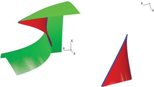
Upon parameter variation, the BN model may display fold¹ bifurcations. At such a bifurcation a mixed stable equilibrium and a mixed unstable equilibrium meet and vanish – or are both born, depending on the direction of the parameter variation. In the bifurcation set of Figure 1 (in $\mathcal{\S }$ 2.3 below) this happens when crossing the green surface. In section 2, we explain this bifurcation set, which gives us a more comprehensive understanding of the model when predicting the complex social phenomenon of segregation. The fold bifurcations turn out to be organized by (dual) cusp bifurcations at the red line in Figure 1, where the two parts of the green surface meet to form a cusp. These parts of the bifurcation set form the discriminant set of a cubic polynomial already obtained in (Haw & Hogan, 2018), the polynomial (8) governing all mixed equilibria. The explanation of these bifurcations is facilitated by the surface in Figure 2, which is the bifurcation diagram detailing how the mixed stable equilibrium born in a fold bifurcation moves over to a second mixed unstable equilibrium to vanish in a second fold bifurcation. The bifurcation set in Figure 1 is completed by a blue surface where the remaining mixed unstable equilibrium merges with the empty neighborhood.

Figure 1. The dynamics of the BN model. Left: the bifurcation set consists of two surfaces separating the three open regions of parameters with the three different behaviours of the system. The smooth surface, blue, is given by (4) and the cuspy surface, green, is the discriminant set given by (9). At the red line, the dark green and light green parts of (9) meet to form a cusp. Right, bottom: the two segregated equilibria $(1,0)$ and $(0,\frac{1}{k})$, both red, attract every point except for the ones on the line separating their basins of attraction and the points on that line tend to the empty equilibrium $(0,0)$, blue. The parameter values $(\mathit{a},\mathit{b},\mathit{k})=(2,0.2,2)$ are between the smooth surface given by (4) and the two co-ordinate planes $\{\mathit{a}=0\}$ and $\{\mathit{b}=0\}$. Right, middle: a saddle, green, has detached from the origin and its stable manifold now separates the basins of attraction of the two segregated equilibria, which still attract all other points. The parameter values $(\mathit{a},\mathit{b},\mathit{k})=(2,2,2)$ are between the smooth and the cuspy surface. Right, top: there is a third attracting equilibrium, red, which is mixed. The two segregated equilibria have basins of attraction bounded by the stable manifolds of the two saddles, both green. These lines also form the boundary of the basin of attraction of the attracting mixed equilibrium. The parameter values $(\mathit{a},\mathit{b},\mathit{k})=(2,8,2)$ are in the third open region of the bifurcation set, the one bounded only by the cuspy surface given by the discriminant (9).

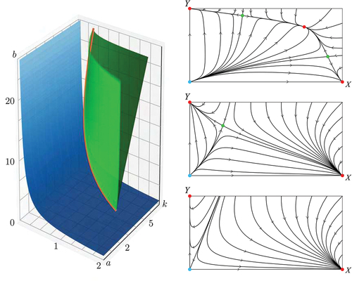
Figure 2. Left: bifurcation diagram showing saddles (green) and stable nodes (red) meeting at the fold line (blue). The surface has $0\le \mathit{X}\le 1$, ends at $\mathit{b}=1$ and we only draw it for $\mathit{k}\ge 1$. Right: for better orientation the bifurcation diagram is rotated to a top view. The saddles are no longer shown (otherwise all of $\mathit{b}\ge 1$ would be green) and the fold line forms a cusp at $(\mathit{k},\mathit{b})=(3,9)$ where it is projected along its vertical tangent.

From the BN model one can construct a model of segregation in two neighborhoods. Discarding the reservoir (think of a small city with only two districts) the $\mathit{X}$– and $\mathit{Y}$–populations move between the two neighborhoods according to their preferences based on tolerance schedules. This is the Two Neighborhood (TN) model of (Haw and Hogan, 2020) treated in section 3. We show in $\mathcal{\S }$ 3.1 how to correct the dynamical system of (Haw and Hogan, 2020) to fully represent the TN model. In $\mathcal{\S }$ 3.2, we then find that all points where the tolerance schedules of neither neighborhood are exceeded form an equilibrium – leading to lines and seas of equilibria for large parts of the parameter space (see Figure 4 in $\mathcal{\S }$ 3.2 below). This makes the model unsuitable for purposes of modeling real-life phenomena, where “unsuitable” has a precise mathematical meaning to be explained now.

Mathematical systems use mathematical concepts to describe real-life phenomena and to predict their behavior. They are rough approximations of the exact relationships describing phenomena in the real world, after focusing on only a single ingredient of the complex relationship between the variables. The BN model describes how segregation in a BN changes as individual tolerances change. It is an abstraction of the particular relationship between individual discriminatory behaviors and segregation, taking into account the tolerances of individuals, while in reality, multiple other factors affect segregation as well. We do not expect the BN model to describe the real world (or parts of it) in an exact fashion. In reality, the real-world system of segregation can be understood as being governed by the model’s equations plus “small” changes and uncertainties. In deterministic systems like the ones used in (Haw & Hogan, 2018, 2020) the latter are given by small perturbations. Such perturbations should be sufficiently small, so small that the dynamics remains qualitatively unchanged under perturbation. The mathematical term for this concept is that of structural stability. Thus, having a structurally stable dynamical system as a model is a necessary condition for drawing conclusions on the real world. This is not possible if the system is not structurally stable. We explain the important concept of structural stability in more detail in $\mathcal{\S }$ 2.3 below, but found it helpful to already here emphasize its impact.

David Haw and John Hogan explicitly formulated the BN model as a dynamical system in their 2018 paper “A dynamical systems model of unorganized segregation.” In their 2020 paper “A dynamical systems model of unorganized segregation in two neighborhoods,” they extended their 2018 dynamical system to create the TN model of self-organized segregation in two neighborhoods. In the present paper, we examine both their 2018 and 2020 papers with the following aims.

1. Perform an in-depth analysis of the 2018 single neighborhood model by assessing in particular the structural stability of the system. Prior to our analysis we additionally correct the scaling used in (Haw & Hogan, 2018) – which, as it turns out, has little consequences and qualitatively the error does not matter.

2. Correct the differential equations for the two-neighborhood model as put forward in (Haw and Hogan, 2020). We conclude that Haw and Hogan’s two neighborhood model is not a suitable model as it leads to dynamical systems that are not structurally stable.

3. Examine the physical implications of the results obtained from both models. We summarize the predictions made possible by the models and point out how stable integration – in the form of trajectories toward a mixed equilibrium – becomes a possibility.

4. Demonstrate that the two-neighborhood model with a reservoir population – as briefly presented in (Haw and Hogan, 2020) – is equivalent to two independent cases of the single-neighborhood model. We also show that the models have no periodic dynamics.

Our mathematical analysis confirms that the dynamics of the BN model is governed by the two surfaces (4) and (9) shown in the left part of Figure 1 (in $\mathcal{\S }$ 2.3 below). We furthermore detail the bifurcations that occur when the parameters are moved across (9) and how this is governed by the surface shown in Figure 2. Our analysis also points out that the reformulation of Haw and Hogan’s (2020) TN model as a dynamical system has non-isolated equilibria, thus preventing structural stability. To achieve aim 3, we detail what our results suggest about how segregation based on individual preferences – in particular on discriminatory behavior – comes about. Allowing a reservoir population in the TN model is proposed as an extension in (Haw and Hogan, 2020, p. 245) and we use the discussion section to show how this simply reduces the TN model to two independent BN models. Prior to this we use the Poincaré index to rule out periodic orbits.

1.2. Outline

We treat two different models – the single neighborhood (BN) model and the two neighborhood (TN) model. These were both introduced in the present section, but for the model itself and for the analysis we use separate sections for each model. Section 2 introduces the basic concepts and theory behind the BN model and presents an overview of the dynamical system. In this section, we also correct the scaling in Haw and Hogan’s (2018) paper. Furthermore, we provide an in-depth qualitative analysis and present our results. Section 3 contains our evaluation of Haw and Hogan’s (2020) TN model. We argue that the given mathematical formulation inaccurately depicts their described model. We consequently introduce a new formulation and perform a qualitative analysis of the system. It turns out that Haw and Hogan’s TN model describes dynamical systems that are not structurally stable. Discussion of the two models and interpretation of the results of our analysis are presented together in section 4. We also prove that both models have no periodic orbits and touch upon Haw and Hogan’s (2020) two-neighborhood model with a reservoir population. Lastly, in section 5, we suggest possible areas of improvement for the single- and the two-neighborhood model and future directions of research.

2. Population dynamics in a bounded neighborhood

To keep the present paper self-contained, we re-build the dynamical system of (Haw & Hogan, 2018) from scratch, also explaining the meaning of the model parameters. We re-do the scaling and explicitly show that reducing the model size from three parameters to two parameters is indeed possible. Our analysis unveils that the model leads to a structurally stable dynamical system – despite the empty neighborhood being a degenerate equilibrium. We also detail the bifurcation diagram, explaining how the BN model can exhibit stable mixed equilibria.

2.1. Model

Individual discriminatory behavior is translated into segregation via tolerance schedules, which are specific to each population. The tolerance schedule of a given population is a function that keeps track of how many members of the population can tolerate how many members of the other population.

The upper limits for the $\mathit{X}$– and $\mathit{Y}$–populations are denoted as $X_{max}$ and $Y_{max}$, respectively. We have $X_{max}=1=\mathit{k}{Y}_{max}$ for the ratio parameter $\mathit{k}\ge 1$ – the ratio of majority to minoriy – and accordingly have $Y_{max}=\frac{1}{k}$. For $\mathit{k}>1$ the $\mathit{Y}$–population is in minority. The phase space (in which the dynamics takes place) is the rectangle

$\mathcal{P}=\left\{\left.(\mathit{X},\mathit{Y})\in {\mathbb{R}}^2\right|0\le \mathit{X}\le 1,0\le \mathit{Y}\le \frac{1}{k}\right\}$

with boundary

$\mathrm{\partial }\mathcal{P}=\left\{(\mathit{X},\mathit{Y})\in \mathcal{P}\left|\mathit{X}=0\mathrm{or}\mathit{X}=1\mathrm{or}\mathit{Y}=0\mathrm{or}\mathit{Y}=\frac{1}{k}\right.\right\}.$

The dynamics in $\mathcal{P}$ is derived from the tolerance schedules $R_X$ of the $\mathit{X}$–population and $R_Y$ of the $\mathit{Y}$–population. These describe the maximal ratios $\frac{Y}{X}$ and $\frac{X}{Y}$ abided by the $\mathit{X}$– and $\mathit{Y}$–populations, respectively (Schelling, 1971). Thus, for

$R_X(\mathit{X})=\frac{Y}{X}\mathrm{and}{R}_Y(\mathit{Y})=\frac{X}{Y}$

the system is in equilibrium. Taking linear tolerance schedules

$R_X(\mathit{X}):=\mathit{a}(1-\mathit{X})\mathrm{and}{R}_Y(\mathit{Y}):=\mathit{b}(1-\mathit{kY})$

with tolerance parameters $\mathit{a}$ and $\mathit{b}$, this results in the parabolas

(1) $\mathit{Y}=\mathit{aX}(1-\mathit{X})\mathrm{and}\mathit{X}=\mathit{bY}(1-\mathit{kY}).$(1)

The $\mathit{X}$–population increases inside the first parabola, i.e. for

$(\mathit{X},\mathit{Y})\in \left\{\left.(\mathit{X},\mathit{Y})\in \mathcal{P}\right|\mathit{Y}<\mathit{aX}(1-\mathit{X})\right\}$

and decreases outside. Similarly, the $\mathit{Y}$–population increases inside the second parabola and decreases where $\mathit{X}>\mathit{bY}(1-\mathit{kY})$.

2.1.1. Dynamical system

The simplest way to encode this as a dynamical system is to put

(2a) $\dot{X}:=\frac{\mathrm{d}X}{\mathrm{d}t}=\mathit{aX}(1-\mathit{X})-\mathit{Y}$(2a)

(2b) $\dot{Y}:=\frac{\mathrm{d}Y}{\mathrm{d}t}=\mathit{bY}(1-\mathit{kY})-\mathit{X}.$(2b)

This makes the empty neighborhood $(\mathit{X},\mathit{Y})=(0,0)$ an equilibrium. However, the dynamics of (2) does not leave the phase space $\mathcal{P}$ invariant. Indeed, for $\mathit{X}=0$, the right-hand side of (2a) is negative (or zero, at the equilibrium) resulting in members of the $\mathit{X}$–population moving out of the BN without living there in the first place. Similarly, the vector field (2) points downward at the boundary part $\{(\mathit{X},\mathit{Y})\in \mathcal{P}|\mathit{Y}=0\}$ of the phase space. Note that (2) does point into $\mathcal{P}$ at the remaining boundary points where $\mathit{X}=1$ or $\mathit{Y}=\frac{1}{k}$.

This problem is remedied by Haw and Hogan (2018) who multiply the right-hand sides of (2a) by $\mathit{X}$ and of (2b) by $\mathit{Y}$, respectively, hence adjusting the dynamical system (2) to

(3a) $\dot{X}=\mathit{X}[\mathit{aX}(1-\mathit{X})-\mathit{Y}]=:\mathit{f}(\mathit{X},\mathit{Y})$(3a)

(3b) $\dot{Y}=\mathit{Y}[\mathit{bY}(1-\mathit{kY})-\mathit{X}]=:\mathit{g}(\mathit{X},\mathit{Y}).$(3b)

This makes the axes $\{(\mathit{X},\mathit{Y})\in \mathcal{P}|\mathit{X}=0\}$ and $\{(\mathit{X},\mathit{Y})\in \mathcal{P}|\mathit{Y}=0\}$ invariant, in particular the corner points $(\mathit{X},\mathit{Y})=(1,0)$ and $(\mathit{X},\mathit{Y})=(0,\frac{1}{k})$ become equilibria.

2.1.2. Preliminary analysis

The Jacobian of the vector field (3) reads as

$\mathit{J}(\mathit{X},\mathit{Y})=\left(\begin{array}{cc}2\mathit{aX}-3\mathit{a}{X}^2-\mathit{Y}& -\mathit{X}\\ -\mathit{Y}& 2\mathit{bY}-3\mathit{kb}{Y}^2-\mathit{X}\end{array}\right).$

Hence, the $\mathit{X}$–segregated equilibrium $(\mathit{X},\mathit{Y})=(1,0)$ is attractive as $\mathit{J}(1,0)$ has negative eigenvalues $-\mathit{a}$ and $-1$. Similarly, $\mathit{J}(0,\frac{1}{k})$ has negative eigenvalues $-\frac{1}{k}$ and $-\frac{b}{k}$ whence the $\mathit{Y}$–segregated equilibrium $(\mathit{X},\mathit{Y})=(0,\frac{1}{k})$ is attractive as well.

However, the adjustment from (2) to (3) has the drawback of turning the empty $(\mathit{X},\mathit{Y})=(0,0)$ into a degenerate equilibrium. Indeed,

$\mathit{J}(0,0)=\left(\begin{array}{cc}0& 0\\ 0& 0\end{array}\right)$

and one has to go to second order to conclude that this equilibrium is repelling for $\mathit{ab}>1$ for the product of the tolerance parameters. In Figure 1 (below in $\mathcal{\S }$ 2.3), we can see that for $\mathit{ab}<1$, the points $(X_0,Y_0)$ on a line in the phase space are attracted to $(0,0)$, i.e. there are initial compositions $(X_0,Y_0)$ for which everybody moves out of the BN. Thus, the qualitative behavior changes when crossing the surface

(4) $\mathit{ab}=1.$(4)

All other equilibria are still obtained by intersecting the parabolas given in (1). In the cases where this results in a single mixed equilibrium $(X_e,Y_e)$ we have

$det\mathit{J}(X_e,Y_e)<0$

and this yields a saddle point, see again Figure 1. As $\mathit{ab}\searrow 1$ the saddle $(X_e,Y_e)$ moves toward $(0,0)$ and reaches it at $\mathit{ab}=1$. The remaining phase portrait in Figure 1 has three mixed equilibria and in this case one of them is attractive, while the other two are again saddles. We continue our analysis in $\mathcal{\S }$ 2.3 and first discuss a possible simplification of the BN model.

2.2. Scaling

Haw and Hogan (2018) propose the scaling

(5) $(\mathit{t},\mathit{X},\mathit{Y})\mapsto (\hat{t},\hat{X},\hat{Y})=(\mathit{at},\mathit{X},\frac{1}{a}\mathit{Y})$(5)

to remove the tolerance parameter $\mathit{a}$ in (3), at the cost of replacing the tolerance $\mathit{b}$ by $\mathit{\beta }=\mathit{ab}$ and the population ratio $\mathit{k}$ by $\mathit{\alpha }=\mathit{ak}$. However, this would turn the Jacobian $\mathit{J}(1,0)$ from

$\left(\begin{array}{cc}-\mathit{a}& -1\\ 0& -1\end{array}\right)\mathrm{into}\left(\begin{array}{cc}-1& -1\\ 0& -1\end{array}\right)$

and thus change the ratio of eigenvalues from $\mathit{a}$ to $1$, while a scaling like (5) is only able to globally scale the eigenvalues (by $\mathit{a}$, the time reparametrization) but not their ratio. Indeed, the scaling (5) turns (3) into

(6a) $\dot{X}=\mathit{X}[\mathit{X}(1-\mathit{X})-\mathit{Y}]$(6a)

(6b) $\dot{Y}=\mathit{Y}[\mathit{bY}(1-\mathit{kY})-\frac{1}{a}\mathit{X}]=\frac{Y}{a}[\mathit{\beta Y}(1-\mathit{\alpha Y})-\mathit{X}]$(6b)

where we have dropped the hats. The extra factor $\frac{1}{a}$ in (6b) is inevitable as now the Jacobian $\mathit{J}(1,0)$ has eigenvalues $-1$ and $-\frac{1}{a}$, so their ratio does remain equal to $\mathit{a}$.

2.2.1. Topological equivalence

The extra factor $\frac{1}{a}$ does not influence the nullclines, whence in particular the equilibria of (3) have positions independent of the value of the tolerance $\mathit{a}$ — provided that we replace the tolerance $\mathit{b}$ by $\mathit{\beta }$ and the ratio $\mathit{k}$ by $\mathit{\alpha }$. In fact, the dynamical systems (3) and

(7a) $\dot{X}=\mathit{X}[\mathit{X}(1-\mathit{X})-\mathit{Y}]$(7a)

(7b) $\dot{Y}=\mathit{Y}[\mathit{abY}(1-\mathit{akY})-\mathit{X}]$(7b)

are topologically equivalent, i.e. qualitatively they display the same dynamics. To prove this we switch to a better suited notation. Let $\mathit{x}=(\mathit{X},\mathit{Y})\in \mathcal{P}$ denote the vector of possible states whence

$\begin{array}{cccc}\mathit{h}:& \mathcal{P}& \to & {\mathbb{R}}^2\\ \mathit{\hspace{0.17em}}& \mathit{x}& \mapsto & (\mathit{f}(\mathit{x}),\mathit{g}(\mathit{x}))\end{array}$

is the vector field in (3). The flow ${\phi }_t$ of $\dot{x}=\mathit{h}(\mathit{x})$ collects all solutions: for every $\mathit{x}\in \mathcal{P}$ and all times $\mathit{t}\in \mathbb{R}$ with ${\phi }_t(\mathit{x})\in \mathcal{P}$ we have that

$\frac{\mathrm{d}}{\mathrm{d}t}{\phi }_t(\mathit{x})=\mathit{h}({\phi }_t(\mathit{x})).$

The trajectory of $\mathit{x}\in \mathcal{P}$ under ${\phi }_t$ is the curve $\{{\phi }_t(\mathit{x})|\mathit{t}\in \mathbb{R}\}$. In cases where going backward in time leads out of the phase space $\mathcal{P}$ we simply restrict time to $\mathit{t}\ge {\tau }_x$ with ${\tau }_x\le 0$ the time at which the trajectory passes through $\mathrm{\partial }\mathcal{P}$. Similarly, let ${\psi }_t$ denote the flow of (7).

Proposition 2.1

There is a homeomorphism $\mathit{\eta }:\mathcal{P}\to \mathcal{P}$ that provides a topological equivalence between the flow ${\phi }_t$ and the flow ${\psi }_t$.

Note that fixing $\mathit{a}$, $\mathit{b}$ and $\mathit{k}$ in (3) yields exactly the values $\mathit{ab}$ and $\mathit{ak}$ in (7b), for which the two systems have the same nullclines.

Proof. To construct the homeomorphism $\mathit{\eta }$, a bijective mapping that is continuous and for which the inverse ${\eta }^{-1}$ is also continuous, we use the so-called stable manifolds

${\mathcal{W}}^s(x_e):=\left\{\mathit{x}\in \mathcal{P}\left|\underset{{\mathit{ }}^{\mathit{t}\to \mathrm{\infty }}}{lim}{\phi }_t(\mathit{x})=x_e\right.\right\}$

of the equilibria $x_e$, consisting of the points attracted to $x_e$. For an attractive equilibrium, this is the basin of attraction, and for a saddle, this is a line separating two basins of attraction. For sufficiently² small radius $\mathit{\delta }>0$ let ${\mathcal{W}}_{\delta }^s(x_e):=\{\mathit{x}\in {\mathcal{W}}^s(x_e)|\parallel \mathit{x}-x_e\parallel =\mathit{\delta }\}$ where $\parallel \mathit{x}\parallel =\sqrt{X^2+Y^2}$ is the Euclidean length of $\mathit{x}=(\mathit{X},\mathit{Y})$. For a saddle, ${\mathcal{W}}_{\delta }^s(x_e)$ consists of two points, one on each arc of the stable manifold, while for the segregated equilibria, ${\mathcal{W}}_{\delta }^s(x_e)$ is a quarter-circle.

For $\mathit{x}\in \mathcal{P}$, we measure the time $\mathit{\tau }(\mathit{x})\in \mathbb{R}$ it takes until the trajectory of $\mathit{x}$ intersects one of the sets ${\mathcal{W}}_{\delta }^s(x_e)$. We then use the flow ${\psi }_t$ to move by $\mathit{t}=-\mathit{\tau }(\mathit{x})$ back in time (or forward if $\mathit{\tau }(\mathit{x})$ is negative), i.e. we let

$\mathit{\eta }(\mathit{x}):=({\psi }_{-\mathit{\tau }(\mathit{x})}\circ {\phi }_{\mathit{\tau }(\mathit{x})})(\mathit{x})={\psi }_{-\mathit{\tau }(\mathit{x})}({\phi }_{\mathit{\tau }(\mathit{x})}(\mathit{x})).$

Outside of the equilibria this defines a diffeomorphism (differentiable with differentiable inverse). By also mapping each equilibrium to itself, we obtain a homeomorphism on all of $\mathcal{P}$ for which ${\psi }_t\circ \mathit{\eta }=\mathit{\eta }\circ {\phi }_t$, i.e. which conjugates the two flows. On trajectories leaving $\mathcal{P}$ at some negative time we then rescale time to ensure that $\mathit{\eta }$ maps $\mathrm{\partial }\mathcal{P}$ to $\mathrm{\partial }\mathcal{P}$.□

In case there are periodic orbits, the period cannot be changed by a conjugating homeomorphism. Originally, this was the reason to weaken the concept of topological conjugacy to that of topological equivalence by allowing for time to be rescaled along the trajectories. Then, occurring periodic orbits can be mapped to each other as well.

2.2.2. The discriminant set

Substituting the first parabola of (1) into the second parabola yields a quartic expression that vanishes at $\mathit{X}=0$ (the equilibrium at the origin) and at the roots of the cubic

(8) $a^2\mathit{bk}{X}^3-2a^2\mathit{bk}{X}^2+\mathit{ab}(1+\mathit{ak})\mathit{X}-\mathit{ab}+1$(8)

(the mixed equilibria). Since omitting the global factor $\frac{1}{a}$ in (6b) does not change the stability type of equilibria, all sections of the bifurcation set with constant tolerance $\mathit{a}=\mathrm{const}.$ of the majority (see Figure 1 in $\mathcal{\S }$ 2.3 below) are scaled versions of each other. In particular, the computation

(9) $b_{\pm }=\frac{9\mathit{ak}-2a^2{k}^2\pm 2\sqrt{\mathit{ak}{(\mathit{ak}-3)}^3}}{\mathit{a}(4-\mathit{ak})}$(9)

by Haw and Hogan (2018) remains valid and still yields the discriminant set of (8) separating the region with $6$ equilibria from the region with $4$ equilibria, see again Figure 1. For $(\mathit{a},\mathit{b},\mathit{k})$ in the discriminant set of (8), i.e. satisfying the Eq. (9(9) $b_{\pm }=\frac{9\mathit{ak}-2a^2{k}^2\pm 2\sqrt{\mathit{ak}{(\mathit{ak}-3)}^3}}{\mathit{a}(4-\mathit{ak})}$(9) ), the dynamical system (3) has $5$ equilibria and a fold (or saddle node) bifurcation takes place, except when additionally $\mathit{ak}=3$ where the saddle undergoes a dual cusp bifurcation (see $\mathcal{\S }$ 2.4 for more details).

The reduction from three parameters $\mathit{a},\mathit{b},\mathit{k}$ to two parameters $\mathit{\alpha },\mathit{\beta }$ simplifies the mathematics, but the interpretation of the product $\mathit{ab}=\mathit{\alpha }$ of tolerances and of the product $\mathit{ak}=\mathit{\beta }$ of tolerance times population ratio is not obvious. For this reason, we avoid in the sequel the use of $\mathit{\alpha }$ and $\mathit{\beta }$ and keep referring to the tolerances $\mathit{a},\mathit{b}$ and the ratio $\mathit{k}$. Note that the systems of Eqs. (6) and (7) do coincide if we put $\mathit{a}=1$, thus making $\mathit{b}$ a kind of relative tolerance parameter.

2.3. Analysis: structural stability

One of the key concepts in the theory of dynamical systems is the concept of structural stability. A vector field $\mathit{h}$ is said to be structurally stable if for all sufficiently small perturbations $h_{\epsilon }$ of $\mathit{h}$ the flows ${\phi }_t^{\epsilon }$ of $h_{\epsilon }$ and ${\phi }_t$ of $\mathit{h}$ are topologically equivalent, i.e. they describe qualitatively similar dynamics.

Having a structurally stable system ensures that the mathematical results obtained for the model under consideration are applicable to the real world. Indeed, it is improbable that the real-world phenomenon of self-organized segregation is exactly described by the vector field (3). If the dynamics of (3) is structurally stable, then for all small perturbations the dynamics behave similarly. It suffices therefore that (3) is close enough. To keep the model’s predictions in line with what is observed in real life, however, one has to improve the model where the phenomena discovered in the dynamics of (3) differ from what is observed in the real world.

Unfortunately, the degeneracy of the equilibrium $\mathit{x}=(0,0)$ prevents the vector field $\mathit{h}=(\mathit{f},\mathit{g})$ in (3) from being structurally stable. Merely subtracting $\mathit{\epsilon }\cdot (\mathit{x},\mathit{y})$ from $\mathit{h}$ yields $h_{\epsilon }(\mathit{x},\mathit{y})=\mathit{h}(\mathit{x},\mathit{y})-\mathit{\epsilon }\cdot (\mathit{x},\mathit{y})$ for which the empty BN $(0,0)$ has the Jacobian

$J_{\epsilon }(0,0)=\left(\begin{array}{cc}-\mathit{\epsilon }& 0\\ 0& -\mathit{\epsilon }\end{array}\right)$

making this an attractive equilibrium for any $\mathit{\epsilon }>0$ and thus preventing a topological equivalence between ${\phi }_t^{\epsilon }$ and ${\phi }_t$. This can be remedied by removing a small disk ${\mathcal{D}}_{\delta }:={\mathcal{D}}_{\delta }(0,0)=\{\mathit{x}\in \mathcal{P}|\parallel \mathit{x}\parallel <\mathit{\delta }\}$ from the phase space $\mathcal{P}$ (or rather a quarter-disk). For $\mathit{ab}>1$ the resulting phase space ${\mathcal{P}}_{\delta }:=\mathcal{P}\mathrm{\setminus }{\mathcal{D}}_{\delta }$ is still invariant under the flow. If additionally $(\mathit{a},\mathit{b},\mathit{k})$ does not satisfy (9), then all remaining equilibria are non-degenerate. The segregated BN $(1,0)$ and $(0,\frac{1}{k})$ are attractive, and in the interior of ${\mathcal{P}}_{\delta }$, there is a saddle and possibly another saddle and a mixed attractive equilibrium.

This mixed stable equilibrium $\mathit{x}=(X_e,Y_e)$, if it exists, is obtained by solving the cubic Eq. (8)(8) $a^2\mathit{bk}{X}^3-2a^2\mathit{bk}{X}^2+\mathit{ab}(1+\mathit{ak})\mathit{X}-\mathit{ab}+1$(8) , which yields unwieldy formulas. However, the qualitative behavior is independent of the exact position of this equilibrium. The boundary of the basin of attraction consists of the stable manifolds of the two saddles.

Proposition 2.2

Let $[0,1]∍\mathit{\lambda }\mapsto (\mathit{a}(\mathit{\lambda }),\mathit{b}(\mathit{\lambda }),\mathit{k}(\mathit{\lambda }))$ be a curve in parameter space that does not cross (4) or (9). Then, for all parameter values on this curve the vector fields (3) are topologically equivalent.

The proposition is formulated in such a way that the situation near the degenerate equilibrium $\mathit{x}=(0,0)$ is included and the proof takes place on the original phase space $\mathcal{P}$.

Proof. It suffices to show that the vector fields for $\mathit{\lambda }=0$ with flow ${\phi }_t$ and $\mathit{\lambda }=1$ with flow ${\psi }_t$ are topologically equivalent. The equilibria and their stability types coincide, and so we can simply adapt the proof of proposition 2.1. The initial diffeomorphism becomes $\mathit{\eta }(\mathit{x})={\psi }_{-\mathit{\tau }(\mathit{x})}(\mathit{\xi }({\phi }_{\mathit{\tau }(\mathit{x})}(\mathit{x})))$ where $\mathit{\xi }$ maps the sets ${\mathcal{W}}_{\delta }^s(x_e)$, $x_e$ the equilibria of ${\phi }_t$, to their counterparts in the flow ${\psi }_t$. Mapping each equilibrium of ${\phi }_t$ to its counterpart in ${\psi }_t$ yields the conjugating homeomorphism. Then, time is again rescaled along trajectories that cut through $\mathrm{\partial }\mathcal{P}$ to ensure that $\mathrm{\partial }\mathcal{P}$ is mapped to $\mathrm{\partial }\mathcal{P}$.□

In particular, for $\mathit{ab}>1$ the dynamical system (3) is structurally stable on ${\mathcal{P}}_{\delta }$ with $\mathit{\delta }$ sufficiently small (as explained below), if $(\mathit{a},\mathit{b},\mathit{k})$ does not satisfy (9). The two possible phase portraits are given in Figure 1. Also, all systems (3) with $\mathit{ab}<1$ have equivalent flows on $\mathcal{P}$, represented by the third phase portrait in Figure 1.

The discriminant set (9) defines the cuspy surface in Figure 1, and Eq. (4)(4) $\mathit{ab}=1.$(4) defines the smooth surface asymptotic to the $(\mathit{a},\mathit{k})$–plane and to the $(\mathit{b},\mathit{k})$–plane. This confirms that Figure 1 gives a faithful representation of the possible dynamics defined by (3), except for the dynamics at the bifurcations. The bifurcation at (4) concerns the degenerate equilibrium $(0,0)$. We follow Haw and Hogan (2018) and do not further consider this empty BN.

When determining the “sufficiently small” size $\mathit{\delta }$ of the disk ${\mathcal{D}}_{\delta }$ to be removed from $\mathcal{P}$ to obtain ${\mathcal{P}}_{\delta }$, we have to make sure that the saddle $x_e$ does not lie in that disk – all while $x_e$ converges to $(0,0)$ as $\mathit{ab}\searrow 1$. To achieve a uniform size $\mathit{\delta }$, we need a uniform bound $\mathit{\beta }\ge {\beta }_0>1$ on $\mathit{\beta }=\mathit{ab}$. Here, we are allowed to choose ${\beta }_0=1.5$ or ${\beta }_0=1.05$ or whatever fixed ${\beta }_0>1$ we find suitable.

2.4. Results: bifurcations

A bifurcation occurs where the system loses structural stability. As shown in $\mathcal{\S }$ 2.2, we may fix the value of the tolerance $\mathit{a}$ of the majority and so for simplicity’s sake we set $\mathit{a}=1$. Then $\mathit{\beta }=\mathit{b}$ is the (relative) tolerance of the minority and $\mathit{\alpha }=\mathit{k}$ is the population ratio, while (4) turns into the equation $\mathit{b}=1$, so we restrict to $\mathit{b}\ge b_0>1$. The discriminant (9) yields a cuspy curve in the $(\mathit{k},\mathit{b})$–plane $\{\mathit{a}=1,\mathit{b}\ge b_0\}$ with apex $(\mathit{k},\mathit{b})=(3,9)$. Here, a dual cusp bifurcation takes place that organizes the whole bifurcation set, see proposition 2.3 below. Fixing $\mathit{a}=1$ the dynamical system (3) becomes

(10a) $\dot{X}=\mathit{X}[\mathit{X}(1-\mathit{X})-\mathit{Y}]$(10a)

(10b) $\dot{Y}=\mathit{Y}[\mathit{bY}(1-\mathit{kY})-\mathit{X}].$(10b)

Next to the empty BN and the two segregated BN there are 1–3 equilibria that are the solutions of a cubic equation, which at the discriminant set defined by

(11) $b_{\pm }=\frac{9\mathit{k}-2k^2\pm 2\sqrt{\mathit{k}{(\mathit{k}-3)}^3}}{4-\mathit{k}}$(11)

turns from having one real solution to having three real solutions.

Proposition 2.3

At $(\mathit{k},\mathit{b})=(3,9)$ the dynamical system (10) undergoes a dual cusp bifurcation.

In particular, when crossing one of the two lines (11) originating from $(\mathit{k},\mathit{b})=(3,9)$ a fold bifurcation takes place where a saddle and a node meet and vanish. That (10) undergoes a dual cusp bifurcation and not a cusp bifurcation means that the third mixed equilibrium (next to the two saddles) is an attractive equilibrium.

Proof. Dividing the cubic (8) by $6\mathit{bk}$ (recall that we restricted to $\mathit{a}=1$) and translating $\mathit{X}\mapsto \mathit{X}+\frac{2}{3}$ puts (8) into the standard form

$\frac{1}{6}{X}^3+\mathit{\mu X}+\mathit{\nu }$

of a cubic, with

$\mathit{\mu }=\frac{1}{6\mathit{k}}-\frac{1}{18}\mathrm{and}\mathit{v}=\frac{1}{6\mathit{bk}}-\frac{1}{18\mathit{k}}+\frac{1}{81}.$

For a negative coefficient of $X^3$ we would have the cusp bifurcation of (Guckenheimer & Holmes, 2002, Figure 7.1.1), but since $\frac{1}{6}>0$, we have the dual cusp bifurcation instead. In particular, two of the equilibria meet and vanish in a fold bifurcation along paths crossing (11)□

Omitting the tolerance parameter $\mathit{a}$ in the picture of the bifurcation set (by putting $\mathit{a}=1$) allows us to draw a bifurcation diagram where we choose the majority $\mathit{X}$ as the vertical co-ordinate. This results in Figure 2 where every point on the green surface corresponds to a saddle and every point on the red surface corresponds to the mixed stable node. Where the two surfaces meet we have fold bifurcations and the dual cusp bifurcation takes place where the fold line has a vertical tangent. Note that the two bifurcation diagrams of (Haw & Hogan, 2018, Figure 4) can be obtained by taking sections $\mathit{k}=\mathrm{const}.$ with $3<\mathit{k}<4$ and $\mathit{k}>4$, respectively.

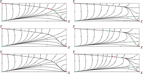
To complement the representation of the dynamics in Figure 1 we give in Figure 3 the phase portraits along a $\mathit{b}$–line with $\mathit{k}=3.5$ fixed. This clearly shows how the attracting equilibrium born in the first fold bifurcation moves over to the other saddle to vanish during the second fold bifurcation. At the apex $(\mathit{k},\mathit{b})=(3,9)$ of the cusp, the phase portrait is similar to the middle one in Figure 1, but with a non-hyperbolic saddle.

Figure 3. Phase portraits for $\mathit{a}=1$, $\mathit{k}=3.5$ and (bottom to top and left to right) $\mathit{b}=11$, $\mathit{b}=b_{-}(3.5)$, $\mathit{b}=12$, $\mathit{b}=16$, $\mathit{b}=b_{+}(3.5)$, $\mathit{b}=17$. Saddles are shown in green, stable nodes in red and non-hyperbolic equilibria in blue.

3. The two-neighborhood model

A possible extension of Schelling’s BN model is to consider two BNs and study the movement of members of each population type between them. In $\mathcal{\S }$ 3.1, we introduce Haw and Hogan’s (2020) dynamical system for the resulting TN model and we explain the inaccuracies of their mathematical formulation. We then correct this formulation to a non-smooth system of differential equations. In $\mathcal{\S }$ 3.2, we perform a qualitative analysis of the corrected system. We concentrate on Case I of (Haw and Hogan, 2020) where both BNs have the same $\mathit{X}$–tolerance schedule $R_X$ and the same $\mathit{Y}$–tolerance schedule $R_Y$. The problems already become apparent in this case, which allows us to simplify the notation. Before summarizing our results we comment on Cases II, III and IV where $R_X$ or $R_Y$ (in Case IV both) become dependent on the BN.

3.1. Model

The sociological model proposed in (Haw and Hogan, 2020) and the mathematical description they give in terms of a dynamical system do not coincide, as we lay out in $\mathcal{\S }$ 3.1.1. In $\mathcal{\S }$ 3.1.2, we therefore change the mathematical description to a dynamical system that does correspond to the sociological model of (Haw and Hogan, 2020). The corrected system is no longer smooth, but nevertheless has a unique solution for every initial condition.

3.1.1. Haw and Hogan’s (2020) formulation

Haw and Hogan (2020) extended Schelling’s BN model by considering two BNs labeled $\mathrm{B}{\mathrm{N}}_1$ and $\mathrm{B}{\mathrm{N}}_2$. For $\mathrm{B}{\mathrm{N}}_i$ the $\mathit{X}$– and $\mathit{Y}$–populations are denoted by $X_i$ and $Y_i$, respectively. They assume that any individual leaving one BN must enter the other BN, and there is no reservoir. The two BNs thus form a closed system and the total $\mathit{X}$– and $\mathit{Y}$–populations are given by $X_{\mathrm{total}}=X_1+X_2=1$ and $Y_{\mathrm{total}}=Y_1+Y_2=\frac{1}{k}$, which yields

(12) $X_2=1-X_1\mathrm{and}{Y}_2=\frac{1}{k}-Y_1$(12)

and in this way we decouple the dynamics of $\mathrm{B}{\mathrm{N}}_1$. Indeed, by differentiating (12) we get

(13) $\frac{\mathrm{d}{X}_2}{\mathrm{d}\mathit{t}}=-\frac{\mathrm{d}{X}_1}{\mathrm{d}\mathit{t}}\mathrm{and}\frac{\mathrm{d}{Y}_2}{\mathrm{d}\mathit{t}}=-\frac{\mathrm{d}{Y}_1}{\mathrm{d}\mathit{t}}$(13)

for $\mathrm{B}{\mathrm{N}}_2$ whence the initially $4$–dimensional system is split into two $2$–dimensional systems, of which one mirrors the dynamics of the other.

Haw and Hogan (2020) make similar assumptions for their TN model as those made by Schelling (1971) for the BN model. A new assumption made for the TN model, however, is that each individual residing in one of the two BNs is only concerned with the population ratio of the BN of residence when deciding whether to remain or leave (Haw and Hogan, 2020, p. 223). Using the same tolerance schedules $R_X$ and $R_Y$ (in the present Case I for both BNs), they then present the system

(14a) ${\dot{X}}_1=\mathit{f}(X_1,Y_1)-\mathit{f}(X_2,Y_2)=\mathit{f}(X_1,Y_1)-\mathit{f}(1-X_1,\frac{1}{k}-Y_1)$(14a)

(14b) ${\dot{Y}}_1=\mathit{g}(X_1,Y_1)-\mathit{g}(X_2,Y_2)=\mathit{g}(X_1,Y_1)-\mathit{g}(1-X_1,\frac{1}{k}-Y_1)$(14b)

governing the dynamics of $\mathrm{B}{\mathrm{N}}_1$. Here $\mathit{f}$ and $\mathit{g}$ are still the functions defined in (3), but now applied in both $\mathrm{B}{\mathrm{N}}_1$ and $\mathrm{B}{\mathrm{N}}_2$. At first glance, the system (14) seems to reflect their described model. Upon closer inspection, however, one can observe that these equations are an incorrect mathematical formulation of the stated model.

Given the assumption that individuals only care about the population ratio of the BN that they currently reside in, the first term $\mathit{f}(X_1,Y_1)$ on the right-hand side of Eq. (14a)(14a) ${\dot{X}}_1=\mathit{f}(X_1,Y_1)-\mathit{f}(X_2,Y_2)=\mathit{f}(X_1,Y_1)-\mathit{f}(1-X_1,\frac{1}{k}-Y_1)$(14a) accounts for the movement of the $X_1$–population in and out of $\mathrm{B}{\mathrm{N}}_1$, subject to the presence of the $Y_1$–population. For $\mathit{f}(X_1,Y_1)\le 0$ this reflects that the members of the $X_1$–population remain in or leave $\mathrm{B}{\mathrm{N}}_1$ according to the tolerance schedule. When $\mathit{f}(X_1,Y_1)>0$, the size of the $Y_1$–population is tolerated by the whole $X_1$–population and all $\mathit{X}$–members remain in $\mathrm{B}{\mathrm{N}}_1$. The situation is most transparent if we additionally assume that $\mathit{f}(X_2,Y_2)=0$, i.e. in $\mathrm{B}{\mathrm{N}}_2$ the $\mathit{X}$–population is in equilibrium. Then ${\dot{X}}_1>0$ and thus $\mathit{f}(X_1,Y_1)>0$ results in an increase in $X_1$. The only reasonable explanation is that the $\mathit{X}$–population in $\mathrm{B}{\mathrm{N}}_1$ is increasing as a result of $\mathit{X}$–members moving in from elsewhere besides $\mathrm{B}{\mathrm{N}}_1$ or $\mathrm{B}{\mathrm{N}}_2$. This, however, contradicts the assumption that we have a closed system with $X_{\mathrm{total}}=X_1+X_2$. Thus, when $\mathit{f}(X_1,Y_1)>0$, Haw and Hogan’s (2020) differential equation for $X_1$ fails to adequately represent their stated model. This similarly applies to $\mathit{f}(X_2,Y_2)$ and to the terms in (14b).

3.1.2. A new dynamical system

For the differential equations to correctly represent the model of (Haw and Hogan, 2020) the following conditions must be met.

1. When $X_1(X_1{R}_X(X_1)-Y_1)>0$, we need to replace $\mathit{f}(X_1,Y_1)$ in (14a) by $0$. Indeed, members of the $\mathit{X}$–population in $\mathrm{B}{\mathrm{N}}_1$ are satisfied with the population ratio and remain in $\mathrm{B}{\mathrm{N}}_1$. As individuals only look at the composition of their own BN and we have a closed system of two BNs, no members of the $\mathit{X}$–population from outside enter $\mathrm{B}{\mathrm{N}}_1$ and there is no contribution resulting from the population ratio in $\mathrm{B}{\mathrm{N}}_1$.

2. Similarly, when $\mathit{f}(X_2,Y_2)>0$, we need to replace $\mathit{f}(X_2,Y_2)$ in (14a) by $0$.

3. When $\mathit{g}(X_1,Y_1)>0$, we need to replace $\mathit{g}(X_1,Y_1)$ in (14b) by $0$.

4. When $\mathit{g}(X_2,Y_2)>0$, we need to replace $\mathit{g}(X_2,Y_2)$ in (14b) by $0$.

Hence, we have to adjust the differential equations (14) according to where the point $(X_1,Y_1,X_2,Y_2)$ lies with respect to the parabolas $Y_i=X_i{R}_X(X_i)$ and $X_i=Y_i{R}_Y(Y_i)$, $\mathit{i}=1,2$. Therefore, we define

(15a) ${\mathcal{F}}_1^{\mathrm{o}\mathrm{u}\mathrm{t}}:=\{\left.(X_1,Y_1)\in \mathcal{P}\right|\mathit{f}(X_1,Y_1)<0\}$(15a)

(15b) ${\mathcal{F}}_1^{\mathrm{i}\mathrm{n}}:=\{\left.(X_1,Y_1)\in \mathcal{P}\right|\mathit{f}(X_1,Y_1)>0\}$(15b)

(15c) ${\mathcal{F}}_2^{\mathrm{o}\mathrm{u}\mathrm{t}}:=\{(X_1,Y_1)\in \mathcal{P}\left|\mathit{f}(1-X_1,\frac{1}{k}-Y_1)<0\right.\}$(15c)

(15d) ${\mathcal{F}}_2^{\mathrm{i}\mathrm{n}}:=\{(X_1,Y_1)\in \mathcal{P}\left|\mathit{f}(1-X_1,\frac{1}{k}-Y_1)>0\right.\}$(15d)

(15e) ${\mathcal{G}}_1^{\mathrm{o}\mathrm{u}\mathrm{t}}:=\{\left.(X_1,Y_1)\in \mathcal{P}\right|\mathit{g}(X_1,Y_1)<0\}$(15e)

(15f) ${\mathcal{G}}_1^{\mathrm{i}\mathrm{n}}:=\{\left.(X_1,Y_1)\in \mathcal{P}\right|\mathit{g}(X_1,Y_1)>0\}$(15f)

(15g) ${\mathcal{G}}_2^{\mathrm{o}\mathrm{u}\mathrm{t}}:=\{(X_1,Y_1)\in \mathcal{P}\left|\mathit{g}(1-X_1,\frac{1}{k}-Y_1)<0\right.\}$(15g)

(15h) ${\mathcal{G}}_2^{\mathrm{i}\mathrm{n}}:=\{(X_1,Y_1)\in \mathcal{P}\left|\mathit{g}(1-X_1,\frac{1}{k}-Y_1)>0\right.\}.$(15h)

The corrected dynamical system then reads as

(16a) ${\dot{X}}_1=F_1(X_1,Y_1)-F_2(X_1,Y_1)$(16a)

(16b) ${\dot{Y}}_1=G_1(X_1,Y_1)-G_2(X_1,Y_1)$(16b)

where

$\begin{array}{ccccc}{F}_1(X_1,Y_1)& :=& \left\{\begin{array}{c}\begin{array}{c}\mathit{f}(X_1,Y_1)\\ 0\\ 0\end{array}\end{array}\right.& \mathrm{when}& \begin{array}{c}(X_1,Y_1)\in {\mathcal{F}}_1^{\mathrm{o}\mathrm{u}\mathrm{t}}\\ \mathit{f}(X_1,Y_1)=0\\ (X_1,Y_1)\in {\mathcal{F}}_1^{\mathrm{i}\mathrm{n}}\end{array}\\ & \\ & \\ F_2(X_1,Y_1)& :=& \left\{\begin{array}{c}\begin{array}{c}\mathit{f}(1-X_1,\frac{1}{k}-Y_1)\\ 0\\ 0\end{array}\end{array}\right.& \mathrm{when}& \begin{array}{c}(X_1,Y_1)\in {\mathcal{F}}_2^{\mathrm{o}\mathrm{u}\mathrm{t}}\\ \mathit{f}(1-X_1,\frac{1}{k}-Y_1)=0\\ (X_1,Y_1)\in {\mathcal{F}}_2^{\mathrm{i}\mathrm{n}}\end{array}\\ \\ & \\ G_1(X_1,Y_1)& :=& \left\{\begin{array}{c}\begin{array}{c}\mathit{g}(X_1,Y_1)\\ 0\\ 0\end{array}\end{array}\right.& \mathrm{when}& \begin{array}{c}(X_1,Y_1)\in {\mathcal{G}}_1^{\mathrm{o}\mathrm{u}\mathrm{t}}\\ \mathit{g}(X_1,Y_1)=0\\ (X_1,Y_1)\in {\mathcal{G}}_1^{\mathrm{i}\mathrm{n}}\end{array}\\ \\ & \\ G_2(X_1,Y_1)& :=& \left\{\begin{array}{c}\begin{array}{c}\mathit{g}(1-X_1,\frac{1}{k}-Y_1)\\ 0\\ 0\end{array}\end{array}\right.& \mathrm{when}& \begin{array}{c}(X_1,Y_1)\in {\mathcal{G}}_2^{\mathrm{o}\mathrm{u}\mathrm{t}}\\ \mathit{g}(1-X_1,\frac{1}{k}-Y_1)=0\\ (X_1,Y_1)\in {\mathcal{G}}_2^{\mathrm{i}\mathrm{n}}.\end{array}\end{array}$

The dynamics of $\mathrm{B}{\mathrm{N}}_2$ can still be obtained from that of $\mathrm{B}{\mathrm{N}}_1$ using (13), which yields

$(X_2(\mathit{t}),Y_2(\mathit{t}))=(1-X_1(\mathit{t}),\frac{1}{k}-Y_1(\mathit{t})).$

Before a qualitative analysis of the new system (16) can be conducted we must first confirm that (16) still has unique solutions (Blanchard et al., 1998, p. 66).

Proposition 3.1

At every point $(X_1,Y_1)\in \mathcal{P}$ the system (16) is locally Lipschitz continuous and thus satisfies the condition for existence and unicity of solutions for all initial conditions $(X_1,Y_1)$.

A function $\mathit{H}:\mathcal{P}\to \mathbb{R}$ is locally Lipschitz continuous if for every $\mathit{x}\in \mathcal{P}$ there exist constants $\mathit{\delta }>0$ and $\mathit{K}$ such that the inequality

$|\mathit{H}(\mathit{y})-\mathit{H}(\mathit{z})|\le \mathit{K}|\mathit{y}-\mathit{z}|$

is satisfied for all $\mathit{y},\mathit{z}\in {\mathcal{D}}_{\delta }(\mathit{x})=\{\mathit{u}\in \mathcal{P}|\parallel \mathit{u}-\mathit{x}\parallel <\mathit{\delta }\}$. This strong form of continuity is satisfied by every continuously differentiable system – take for the Lipschitz constant $\mathit{K}$ a local bound on the derivative.

Proof. As linear combinations of locally Lipschitz continuous functions are again locally Lipschitz continuous, we only treat $F_1$ (the arguments for $F_2,G_1$ and $G_2$ are similar). On ${\mathcal{F}}_1^{\mathrm{o}\mathrm{u}\mathrm{t}}$ and ${\mathcal{F}}_1^{\mathrm{i}\mathrm{n}}$ the function $F_1$ is continuously differentiable and therefore locally Lipschitz continuous with $\mathit{K}$ an upper bound of the length $\parallel F_1^{\prime }\parallel$ of the total derivative of $F_1$ on ${\mathcal{D}}_{\delta }(\mathit{x})$. At a point $\mathit{x}=(X_1,Y_1)$ on the parabola $Y_1=X_1{R}_X(X_1)$, the function $F_1$ is still continuous, and we use that the ingredient $\mathit{f}$ of $F_1$ is continuously differentiable everywhere, hence with a Lipschitz constant $\mathit{K}$ in $\mathit{x}$. The inequality

$|\mathit{f}(\mathit{y})-\mathit{f}(\mathit{z})|\le \mathit{K}|\mathit{y}-\mathit{z}|$

for $\mathit{y},\mathit{z}\in {\mathcal{D}}_{\delta }(\mathit{x})$ becomes

$|F_1(\mathit{y})-F_1(\mathit{z})|\le \mathit{K}|\mathit{y}-\mathit{z}|$

when both $\mathit{y}$ and $\mathit{z}$ are in ${\mathcal{F}}_1^{\mathrm{o}\mathrm{u}\mathrm{t}}$, while when both $\mathit{y}$ and $\mathit{z}$ are in $\overline{{\mathcal{F}}_1^{\mathrm{i}\mathrm{n}}}$ the latter simply reads as $|0-0|\le \mathit{K}|\mathit{y}-\mathit{z}|$. When $\mathit{y}\in \overline{{\mathcal{F}}_1^{\mathrm{i}\mathrm{n}}}$ and $\mathit{z}\in {\mathcal{F}}_1^{\mathrm{o}\mathrm{u}\mathrm{t}}$, we have that

$|F_1(\mathit{y})-F_1(\mathit{z})|=|0-\mathit{f}(\mathit{z})|\le |\mathit{f}(\mathit{y})-\mathit{f}(\mathit{z})|\le \mathit{K}|\mathit{y}-\mathit{z}|$

as $\mathit{f}(\mathit{y})\ge 0$ and $\mathit{f}(\mathit{z})<0$ (and similarly when $\mathit{y}\in {\mathcal{F}}_1^{\mathrm{o}\mathrm{u}\mathrm{t}}$ and $\mathit{z}\in \overline{{\mathcal{F}}_1^{\mathrm{i}\mathrm{n}}}$).□

Note that during the proof we replaced ${\mathcal{F}}_1^{\mathrm{i}\mathrm{n}}$ by its closure $\overline{{\mathcal{F}}_1^{\mathrm{i}\mathrm{n}}}$ to include the points on the parabola $Y_1=X_1{R}_X(X_1)$.

3.2. Analysis

Again the scaling (5) allows $\mathit{a}=1$ to be achieved in (16), at the cost of replacing $(\mathit{k},\mathit{b})$ by $(\mathit{\alpha },\mathit{\beta })=(\mathit{ak},\mathit{ab})$ and multiplying the right-hand side in (16b) by $\frac{1}{a}$. Haw and Hogan (2020) scale time by $\frac{1}{k}$ instead – effectively this means an extra scaling of time by $\frac{1}{\alpha }$ and correspondingly the vector field is multiplied by $\mathit{\alpha }$. The extra scaling of time by $\frac{1}{\alpha }$ has the advantage that

$\mathit{\alpha f}(X_2,Y_2)=(1-X_1)[\mathit{\alpha }{X}_1(1-X_1)-(1-\mathit{\alpha }{Y}_1)]$

and

$\mathit{\alpha g}(X_2,Y_2)=\frac{1}{a}(1-\mathit{\alpha }{Y}_1)[\mathit{\beta }{Y}_1(1-\mathit{\alpha }{Y}_1)-(1-X_1)]$

have no $\mathit{\alpha }$ in the denominator, so we keep it. For the nullclines, the parameters are again reduced from $(\mathit{a},\mathit{b},\mathit{k})$ to $(\mathit{\alpha },\mathit{\beta })$. By taking the tolerance $\mathit{a}=1$ we have $\mathit{\alpha }=\mathit{k}$ keeping its interpretation of the majority–minority ratio, while $\mathit{\beta }=\mathit{b}$ can be interpreted as the relative tolerance of the $\mathit{Y}$–population (with respect to the $\mathit{X}$–population).

3.2.1. Equilibria

The segregated $(1,0)$, $(0,\frac{1}{\alpha })$ have both right hand sides in (16) read as $0-0$ and are always equilibria, even though the vector field is not differentiable on the union of the four parabolas. On ${\mathcal{F}}_1^{\mathrm{o}\mathrm{u}\mathrm{t}}\cap {\mathcal{F}}_2^{\mathrm{o}\mathrm{u}\mathrm{t}}\cap {\mathcal{G}}_1^{\mathrm{o}\mathrm{u}\mathrm{t}}\cap {\mathcal{G}}_2^{\mathrm{o}\mathrm{u}\mathrm{t}}$ the vector field (16) coincides with (14) and the analysis of (Haw and Hogan, 2020) remains valid. In particular, the mixed $(\frac{1}{2},\frac{1}{2\mathit{\alpha }})$ is also always an equilibrium. Additional equilibria $(X_e,Y_e)$ can be obtained from the roots $X_e=X_1$ of a polynomial $p_6(X_1)$ of degree $6$. These $3$–$9$ equilibria are the intersections of the two cubic nullclines computed by Haw and Hogan (2020).

The cubic $X_1$–nullcline always stays inside ${\mathcal{F}}_1^{\mathrm{o}\mathrm{u}\mathrm{t}}\cap {\mathcal{F}}_2^{\mathrm{o}\mathrm{u}\mathrm{t}}$ — except if the parabolas $Y_1=X_1(1-X_1)$ and $\mathit{\alpha }{Y}_1=1-\mathit{\alpha }{X}_1(1-X_1)$ overlap (so $\overline{{\mathcal{F}}_1^{\mathrm{i}\mathrm{n}}}$ and $\overline{{\mathcal{F}}_2^{\mathrm{i}\mathrm{n}}}$ intersect) and the right-hand side of (16a) is identically zero on $\overline{{\mathcal{F}}_1^{\mathrm{i}\mathrm{n}}}\cap \overline{{\mathcal{F}}_2^{\mathrm{i}\mathrm{n}}}$. Then, the part of the cubic $Y_1$–nullcline inside $\overline{{\mathcal{F}}_1^{\mathrm{i}\mathrm{n}}}\cap \overline{{\mathcal{F}}_2^{\mathrm{i}\mathrm{n}}}$ is a line of equilibria. Similarly, where the parabolas $X_1=\mathit{\beta }{Y}_1(1-\mathit{\alpha }{Y}_1)$ and $X_1=1-\mathit{\beta }{Y}_1(1-\mathit{\alpha }{Y}_1)$ overlap, the part of the cubic $X_1$–nullcline inside $\overline{{\mathcal{G}}_1^{\mathrm{i}\mathrm{n}}}\cap \overline{{\mathcal{G}}_2^{\mathrm{i}\mathrm{n}}}$ is a line of equilibria. If both ${\mathcal{F}}_1^{\mathrm{i}\mathrm{n}}\cap {\mathcal{F}}_2^{\mathrm{i}\mathrm{n}}\ne \mathrm{\varnothing }$ and ${\mathcal{G}}_1^{\mathrm{i}\mathrm{n}}\cap {\mathcal{G}}_2^{\mathrm{i}\mathrm{n}}\ne \mathrm{\varnothing }$, then the common intersection ${\mathcal{F}}_1^{\mathrm{i}\mathrm{n}}\cap {\mathcal{F}}_2^{\mathrm{i}\mathrm{n}}\cap {\mathcal{G}}_1^{\mathrm{i}\mathrm{n}}\cap {\mathcal{G}}_2^{\mathrm{i}\mathrm{n}}$ is even a “sea of equilibria” with its boundary formed by parts of the parabolas. All such infinite sets of equilibria are centered at the mixed equilibrium $(\frac{1}{2},\frac{1}{2\mathit{\alpha }})$.

In particular, where valid the polynomial $p_6(X_1)$ is never zero and where there are only finitely many equilibria, these are the segregated $(1,0)$, $(0,\frac{1}{\alpha })$, both attracting and the mixed $(\frac{1}{2},\frac{1}{2\mathit{\alpha }})$, a saddle (see $\mathcal{\S }$ 3.2.2 for more details). Before the bifurcations found by Haw and Hogan (2020) can occur, the saddle has already exploded into an infinite set of equilibria. Note that the $X_1$– and $Y_1$–axes are no longer nullclines of the system whence the empty $(0,0)$ is no longer an equilibrium, unlike in the single BN model.

The existence of a line or a sea of equilibria immediately shows that for such parameter values, the system (16) is not structurally stable. Let us therefore compute the parameter values $(\mathit{\alpha },\mathit{\beta })$ for which the parabolas start overlapping. Equating

$\mathit{\alpha }{X}_1(1-X_1)=1-\mathit{\alpha }{X}_1(1-X_1)$

yields

$X_1=\frac{1}{2}\pm \frac{1}{2}\sqrt{\frac{\mathit{\alpha }-2}{\alpha }},$

so the change occurs at $\mathit{\alpha }=2$. Similarly,

$\mathit{\beta }{Y}_1(1-\mathit{\alpha }{Y}_1)=1-\mathit{\beta }{Y}_1(1-\mathit{\alpha }{Y}_1)$

yields

$Y_1=\frac{1}{2\mathit{\alpha }}\pm \frac{1}{2\mathit{\alpha }}\sqrt{\frac{\mathit{\beta }-2\mathit{\alpha }}{\beta }}$

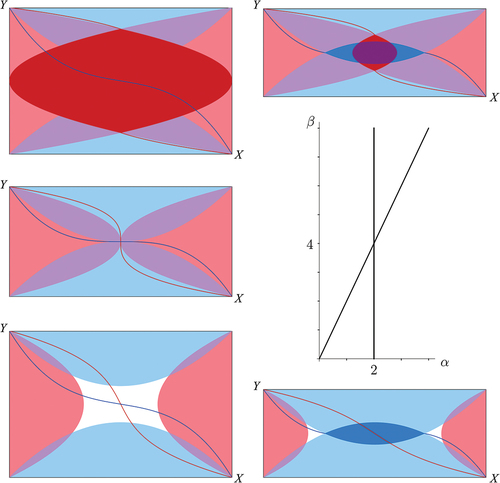
and the change occurs at $\mathit{\beta }=2\mathit{\alpha }$. We therefore have the bifurcation set shown in Figure 4.

Figure 4. Bifurcation set of (16) in the $(\mathit{\alpha },\mathit{\beta })$–plane (or, equivalently, for tolerance $\mathit{a}=1$ in the $(\mathit{k},\mathit{b})$–plane). Counterclockwise (starting top right) the five pictures of nullclines have parameter values $(\mathit{\alpha },\mathit{\beta })=(2.5,6),(1.5,6),(2,4),(1.5,2),(2.5,2)$. In blue the cubic $X_1$–nullcline (dark) and the regions ${\mathcal{F}}_1^{\mathrm{i}\mathrm{n}}$, ${\mathcal{F}}_2^{\mathrm{i}\mathrm{n}}$ (light) and in red the cubic $Y_1$–nullcline (dark) and the regions ${\mathcal{G}}_1^{\mathrm{i}\mathrm{n}}$, ${\mathcal{G}}_2^{\mathrm{i}\mathrm{n}}$ (light). Where an ${\mathcal{F}}_i^{\mathrm{i}\mathrm{n}}$ and a ${\mathcal{G}}_j^{\mathrm{i}\mathrm{n}}$ intersect the colours mix to light purple. Only in the two top pictures ${\mathcal{G}}_1^{\mathrm{i}\mathrm{n}}\cap {\mathcal{G}}_2^{\mathrm{i}\mathrm{n}}\ne \mathrm{\varnothing }$ and only in the top right and bottom right pictures ${\mathcal{F}}_1^{\mathrm{i}\mathrm{n}}\cap {\mathcal{F}}_2^{\mathrm{i}\mathrm{n}}\ne \mathrm{\varnothing }$. Correspondingly, the top right picture features a (dark purple) sea of equilibria ${\mathcal{F}}_1^{\mathrm{i}\mathrm{n}}\cap {\mathcal{F}}_2^{\mathrm{i}\mathrm{n}}\cap {\mathcal{G}}_1^{\mathrm{i}\mathrm{n}}\cap {\mathcal{G}}_2^{\mathrm{i}\mathrm{n}}$. The middle left picture is also not structurally stable as small perturbations can lead to both the bottom left picture as to one of the other three pictures (the latter are clearly not structurally stable, displaying infinitely many equilibria).

3.2.2. Phase portraits

The adjustment from (14a) to (16a) is most severe on ${\mathcal{F}}_1^{\mathrm{i}\mathrm{n}}\cap {\mathcal{F}}_2^{\mathrm{i}\mathrm{n}}$, where the parabolas intersect. For $(X_1,Y_1)\in {\mathcal{F}}_1^{\mathrm{i}\mathrm{n}}\cap {\mathcal{F}}_2^{\mathrm{o}\mathrm{u}\mathrm{t}}$ the term $\mathit{f}(X_1,Y_1)$ is positive and gets adjusted to zero, but the term $-\mathit{f}(X_2,Y_2)$ is also positive, so the right-hand side of (16a) remains positive. Similarly, on ${\mathcal{F}}_1^{\mathrm{o}\mathrm{u}\mathrm{t}}\cap {\mathcal{F}}_2^{\mathrm{i}\mathrm{n}}$ the right-hand side of (16a) remains negative. On ${\mathcal{F}}_1^{\mathrm{o}\mathrm{u}\mathrm{t}}\cap {\mathcal{F}}_2^{\mathrm{o}\mathrm{u}\mathrm{t}}$ the cubic $X_1$–nullcline separates the positive values below from the negative values above. Thus, we have the minor adjustment that the positive values below the $X_1$–nullcline become smaller (but remain positive) within ${\mathcal{F}}_1^{\mathrm{i}\mathrm{n}}\cap {\mathcal{F}}_2^{\mathrm{o}\mathrm{u}\mathrm{t}}$ and that the negative values above the $X_1$–nullcline become larger (but remain negative) within ${\mathcal{F}}_1^{\mathrm{o}\mathrm{u}\mathrm{t}}\cap {\mathcal{F}}_2^{\mathrm{i}\mathrm{n}}$. The major adjustment is that the $X_1$–nullcline gets broadened to $\overline{{\mathcal{F}}_1^{\mathrm{i}\mathrm{n}}}\cap \overline{{\mathcal{F}}_2^{\mathrm{i}\mathrm{n}}}$ where the parabolas intersect. The same applies mutatis mutandis to the adjustment from (14b) to (16b).

Proposition 3.2

For the adjusted system (16) the segregated equilibria $(1,0)$ and $(0,\frac{1}{\alpha })$ are attractive.

Haw and Hogan (2020) could simply compute the Jacobians in these points to prove that these are both stable nodes for (14). The system (16) is not differentiable at the segregated equilibria.

Proof. We focus on $(1,0)$ as the argument for $(0,\frac{1}{\alpha })$ is similar. Take $\mathit{\delta }>0$ so small that

${\mathcal{D}}_{\delta }(1,0)\subseteq {\mathcal{F}}_2^{\mathrm{o}\mathrm{u}\mathrm{t}}\cap {\mathcal{G}}_1^{\mathrm{o}\mathrm{u}\mathrm{t}}$

and consider the vector field (16) restricted to ${\mathcal{D}}_{\delta }(1,0)$. Between the two nullclines, the vector field points downward right, while on the two nullclines, the vector field points to the right and points downwards, respectively. Below the $X_1$–nullcline the vector field points upward right and all trajectories reach the $X_1$–nullcline in finite time. To the right of the $Y_1$–nullcline the vector field points downward left and all trajectories reach the $Y_1$–nullcline in finite time. Hence, all initial conditions $(X_1,Y_1)\in {\mathcal{D}}_{\delta }(1,0)$ have trajectories that tend to $(1,0)$ as $\mathit{t}\to \mathrm{\infty }$.□

The basins of attraction of the segregated equilibria are clearly larger than a mere disk ${\mathcal{D}}_{\delta }$, see e.g. Figure 5, left. Within ${\mathcal{F}}_1^{\mathrm{o}\mathrm{u}\mathrm{t}}\cap {\mathcal{F}}_2^{\mathrm{o}\mathrm{u}\mathrm{t}}\cap {\mathcal{G}}_1^{\mathrm{o}\mathrm{u}\mathrm{t}}\cap {\mathcal{G}}_2^{\mathrm{o}\mathrm{u}\mathrm{t}}$ the Jacobian of (16) reads as

(17) $\mathit{J}(X_1,Y_1)=\left(\begin{array}{cc}-(1+\mathit{\alpha })+6\mathit{\alpha }{X}_1(1-X_1)& -\mathit{\alpha }\\ -\frac{1}{a}& \frac{1}{a}[-(\mathit{\alpha }+\mathit{\beta })+6\mathit{\alpha \beta }{Y}_1(1-\mathit{\alpha }{Y}_1)]\end{array}\right)$(17)

Figure 5. Phase portraits of (16) for $(\mathit{\alpha },\mathit{\beta })=(1.5,2)$, left, and for $(\mathit{\alpha },\mathit{\beta })=(2,4)$, right—the choice $\mathit{a}=1$ implies $\mathit{k}=\mathit{\alpha }$ and $\mathit{b}=\mathit{\beta }$, respectively. The left phase portrait is structurally stable while the right phase portrait is not – a fact that can be derived only by looking at small perturbations (see figure 4). Note that both phase portraits are invariant under a rotation of ${180}^{\circ }$—the dynamics of $\mathrm{B}{\mathrm{N}}_2$ coincides with that of $\mathrm{B}{\mathrm{N}}_1$.

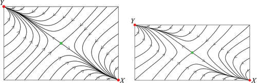
where the global factor $\frac{1}{a}$ in the second row corrects the scaling error of Haw and Hogan (2018, 2020). The determinant

$det\mathit{J}(\frac{1}{2},\frac{1}{2\mathit{\alpha }})=\frac{-1}{4\mathit{a}}[2{\alpha }^2+(2-\mathit{\alpha })\mathit{\beta }]$

is negative for $\mathit{\alpha }<2$ whence the isolated mixed equilibrium is a saddle. This yields for $(\mathit{\alpha },\mathit{\beta })$ with $\mathit{\beta }<2\mathit{\alpha }<4$ the phase portrait in Figure 5, left. The basins of attraction of $(1,0)$ and $(0,\frac{1}{\alpha })$ are separated by the stable manifold of the mixed equilibrium. Recall that for $\mathit{\beta }>2\mathit{\alpha }$ we have that ${\mathcal{G}}_1^{\mathrm{i}\mathrm{n}}\cap {\mathcal{G}}_2^{\mathrm{i}\mathrm{n}}\ne \mathrm{\varnothing }$ and $(\frac{1}{2},\frac{1}{2\mathit{\alpha }})$ is not isolated.

For $(\mathit{\alpha },\mathit{\beta })$ on the boundary $\mathit{\beta }=2\mathit{\alpha }$ the vector field (16) is only Lipschitz continuous in $(\frac{1}{2},\frac{1}{2\mathit{\alpha }})$. Taking for $\mathit{\beta }<2\mathit{\alpha }<4$ the limit $(\mathit{\alpha },\mathit{\beta })\to (\mathit{\alpha },2\mathit{\alpha })$ shows that the isolated mixed equilibrium keeps behaving like a saddle when the limit is reached. This is also true when taking for $\mathit{\beta }<2\mathit{\alpha }<4$ the limit $(\mathit{\alpha },\mathit{\beta })\to (2,\mathit{\beta })$. In particular, for $(\mathit{\alpha },\mathit{\beta })=(2,4)$, the mixed equilibrium is isolated and behaves like a saddle, see Figure 5, right.

When $\mathit{\beta }>2\mathit{\alpha }$ (and $\mathit{\alpha }<2$) the vector field is differentiable on ${\mathcal{G}}_1^{\mathrm{i}\mathrm{n}}\cap {\mathcal{G}}_2^{\mathrm{i}\mathrm{n}}$, but the entries in the second row of (17) have been replaced by $0$. This yields a zero eigenvalue, corresponding to the line of equilibria. When $\mathit{\alpha }>2$ (but $\mathit{\beta }<2\mathit{\alpha }$) the first row of (17) consists of zeroes, corresponding to the line of equilibria in $\overline{{\mathcal{F}}_1^{\mathrm{i}\mathrm{n}}}\cap \overline{{\mathcal{F}}_2^{\mathrm{i}\mathrm{n}}}$. When $\mathit{\beta }>2\mathit{\alpha }>4$, the equilibria in ${\mathcal{F}}_1^{\mathrm{i}\mathrm{n}}\cap {\mathcal{F}}_2^{\mathrm{i}\mathrm{n}}\cap {\mathcal{G}}_1^{\mathrm{i}\mathrm{n}}\cap {\mathcal{G}}_2^{\mathrm{i}\mathrm{n}}$ have zero Jacobian (both eigenvalues vanish). Note that on the boundaries of these lines and sea of equilibria, the vector field (16) still vanishes, but is not differentiable.

3.2.3. Different tolerance schedules

In (Haw and Hogan, 2020) the vector field (14) has $\mathit{f}$ and $\mathit{g}$ depend on the BN, with $\mathit{f}(X_1,Y_1)$ replaced by

(18a) $f_1(X_1,Y_1):=X_1[a_1{X}_1(1-X_1)-Y_1]$(18a)

and $\mathit{f}(X_2,Y_2)$ replaced by

(18b) $f_2(X_2,Y_2):=X_2[a_2{X}_2(1-X_2)-Y_2].$(18b)

Thus, $\mathrm{B}{\mathrm{N}}_1$ and $\mathrm{B}{\mathrm{N}}_2$ have different tolerance parameters $a_1$ and $a_2$, respectively. A scaling like (5) cannot change their ratio, which is denoted by

$\mathit{\gamma }:=\frac{a_2}{a_1}.$

Similarly, $\mathit{g}(X_1,Y_1)$ and $\mathit{g}(X_2,Y_2)$ get replaced by

(18c) $g_1(X_1,Y_1):=Y_1[b_1{Y}_1(1-\mathit{k}{Y}_1)-X_1]$(18c)

(18d) $g_2(X_2,Y_2):=Y_2[b_2{Y}_2(1-\mathit{k}{Y}_2)-X_2]$(18d)

with different tolerance parameters $b_1$ and $b_2$, while the population ratio $\mathit{k}=\frac{{\mathit{X}}_{\mathrm{total}}}{Y_{\mathrm{total}}}$ remains the same for both BNs. Scaling both $Y_1$ and $Y_2$ by $\frac{1}{a_1}$ but $\mathit{t}$ by $\frac{1}{k}$ leads³ to

$\mathit{\alpha }:=a_1\mathit{k},{\beta }_1:=a_1{b}_1,{\beta }_2:=a_1{b}_2$

with again an extra factor $\frac{1}{a_1}$ in the ${\dot{Y}}_1$–equation, but otherwise reducing parameters from $(a_1,a_2,b_1,b_2,\mathit{k})$ to $(\mathit{\alpha },{\beta }_1,{\beta }_2,\mathit{\gamma })$.

Generalizing (16) to (18) does not change the fundamental problem. While the symmetry line reflecting the parabola $f_1=0$ into the parabola $f_2=0$ may shift up or down, on their intersection the right-hand side of the ${\dot{X}}_1$–equation still has to vanish. The situation is similar for $g_1=0$, $g_2=0$ and the ${\dot{Y}}_1$–equation.

The bifurcations to further equilibria found in (Haw and Hogan, 2020) all require the cubic $X_1$–nullcline to evolve extrema. However, before this can happen the $X_1$–nullcline must have a horizontal inflection point, after which the parabolas $f_1=0$ and $f_2=0$ start to intersect. This similarly applies for the $Y_1$–nullcline. Thus, before the bifurcations detailed in (Haw and Hogan, 2020) can take place, the adjustment of the vector field has already led to lines and seas of equilibria. Note that an intersection of parabolas no longer necessarily leads to infinitely many equilibria, as the “other” nullcline is no longer enforced to pass through, but a bifurcation does require the “other” nullcline to pass through the intersection of parabolas.

Again, such dynamics is not structurally stable. Also, for tolerance parameters dependent on the BN, the only phase portraits with finitely many equilibria have the two attracting segregated equilibria and a mixed saddle. As already explained by Haw and Hogan (2020), the saddle is no longer fixed at $(\frac{1}{2},\frac{1}{2\mathit{\alpha }})$, though.

3.2.4. Results

The corrected system (16) fails to be everywhere differentiable, but in a mild way. It is still locally Lipschitz continuous, and hence for every initial condition, there is a unique solution – all these together form the flow of (16). Mutatis mutandis this applies to the system with right-hand sides (18) as well.

Our qualitative analysis yields a bifurcation set in Figure 4, with three of the four open regions displaying dynamics that is not structurally stable. For the system (14), Haw and Hogan (2020) were able to find bifurcations to attractive mixed equilibria, and we discuss in the concluding section 5 that it might be worthwhile to change the sociological model in such a way that (14) becomes a valid description.

A word of warning on the use of structural stability: for parameter values like $(\mathit{\alpha },\mathit{\beta })=(1.5,2)$ deep inside the structurally stable region of Figure 4, the smallness requirement on perturbations is not particularly restrictive. However, the closer $(\mathit{\alpha },\mathit{\beta })$ is chosen to the boundary of that region, the smaller the perturbations are allowed to be. This phenomenon is not specific to the structurally stable part of the TN model, but is “built-in” to the definition of structural stability: for a perturbation to be sufficiently small may mean very small.

4. Discussion

We have achieved a complete understanding of the dynamics defined by (3) and by (16). We explained how the dynamics of (3) can be made structurally stable when the product of tolerances $\mathit{ab}\ge {\beta }_0$ is above a threshold ${\beta }_0>1$ and detailed the occurring bifurcations. The system (16) is not structurally stable for $(\mathit{\alpha },\mathit{\beta })$ outside the small wedge $\{0<\mathit{\beta }<2\mathit{\alpha }<4\}$. For $(\mathit{\alpha },\mathit{\beta })$ inside the wedge, the dynamics consists of two stable segregated equilibria, with basins of attraction separated by the stable manifold of a mixed saddle, see Figure 5, left.

4.1. Interpretation

The BN model is very simple, and this is not only its weakness but also its strength. Among the weaknesses is the choice of the phase space

$\mathcal{P}=[0,1]\times [0,\frac{1}{k}]$

where the relative size $Y_{max}=\frac{1}{k}{X}_{max}$ of the minority population is built into the model in such a way that there are immediate further consequences. For instance, where the segregated equilibrium $(1,0)$ may grant one place per member of the $\mathit{X}$–population, the segregated equilibrium $(0,\frac{1}{k})$ then grants on average $\mathit{k}$ places to members of the $\mathit{Y}$–population. The capacity of the BN is simply not part of the model as the $\mathit{X}$–slots and the $\mathit{Y}$–slots are filled independently; the interdependence in (3) solely stems from the tolerances.

Another weakness of the BN model is that (2) not leaving $\mathcal{P}$ invariant is remedied by simple multiplication with $\mathit{X}$ and $\mathit{Y}$, respectively. This turns the empty $(0,0)$ into a degenerate equilibrium. The model still captures that the composition of a BN with a low number of residents does not exceed the tolerance of most individuals of either population. Consequently, individuals start moving in when the initial composition of the BN is close to the origin. The composition then changes over time as residents remain or leave, depending on whether their tolerances are exceeded. Eventually, the BN reaches a composition that corresponds to a stable node (or, exceptionally, to a saddle).

Two stable nodes present for all parameter values are $(1,0)$ and $(0,\frac{1}{k})$. This shows that regardless of how tolerant the two populations are, the BN can segregate. For parameter values outside the cuspy region, the initial composition merely decides whether the BN segregates to an all $\mathit{X}$–population or an all $\mathit{Y}$–population – and the precise parameter values determine which basin of attraction is larger (but that is already a quantitative statement that might be out of the scope of the BN model).

For parameter values inside the cuspy region, there is a third stable node, with a mixed population. The precise position of the parameters determines the position of the two saddles (and of the mixed stable node) and thus determines the sizes of the three basins of attraction. The node the dynamics leads to depends on the basin of attraction the initial composition lies in. Where the trajectory passes close to the stable manifold of a saddle, BN tipping can be achieved by pushing the state $(\mathit{X}(\mathit{t}),\mathit{Y}(\mathit{t}))$ of the system to the other side of that stable manifold.

An interesting prediction made by the BN model is that a stable node corresponding to a mixed BN only exists for parameter values inside the cuspy region. It is thus not sufficient to simply increase the values of the tolerance parameters to obtain a mixed BN. Instead, such an increase has to be achieved in such a way that the parameter values enter the cuspy region and one still has to ensure that the trajectory is in the basin of attraction of the mixed node. The phase portraits in Figure 3 convincingly show how increasing the tolerance $\mathit{b}$ of the minority $(\mathit{Y})$ — with population ratio $\mathit{k}$ and tolerance $\mathit{a}$ of the majority $(\mathit{X})$ fixed – first leads to the creation of a mixed stable node and, as the tolerance $\mathit{b}$ is increased even further, to the annihilation of that mixed stable node. Ultimately, the basin of attraction for the segregated stable node of an all $\mathit{Y}$ population is increased, while the basin of attraction for an all $\mathit{X}$ population has decreased. Note that the mathematical assumption that the tolerance $\mathit{a}$ remains fixed during the increase in the tolerance $\mathit{b}$ probably does not reflect real life and $\mathit{a}$ might increase as well, keeping the system in the cuspy region.

The TN model on $\mathcal{P}$ with $\mathit{\beta }<2\mathit{\alpha }<4$ has dynamics rather similar (although not topologically equivalent) to the BN model on ${\mathcal{P}}_{\delta }$ with parameter values outside the cuspy region (but satisfying $\mathit{ab}>1$). The population trajectories lead to neighborhood compositions where $\mathrm{B}{\mathrm{N}}_1$ is segregated with one type of population and $\mathrm{B}{\mathrm{N}}_2$ is likewise segregated with the other type of population. The initial composition of the neighborhoods merely decides which particular population each BN is eventually composed of (unless we have an exceptional initial composition on the stable manifold of the saddle). The model is not well fitted to describe real-world scenarios that have parameter values $(\mathit{\alpha },\mathit{\beta })$ with $\mathit{\alpha }\ge 2$ or $\mathit{\beta }\ge 2\mathit{\alpha }$.

4.2. Further results

We include in this discussion section two further results that concern both models. One result is that there are no periodic orbits; the only orbits for which the past completely stays inside the phase space are the $3$ or $5$ equilibria and the $2$ or $4$ heteroclinic orbits from saddles to attractive equilibria. All other orbits leave the phase space ${\mathcal{P}}_{\delta }$ (for the BN model), respectively $\mathcal{P}$ (for the TN model) in backward time. The second result concerns a two-neighborhood model with reservoir – but without direct movements between the neighborhoods. Such a model is brought back to two individual BN models.

4.2.1. Absence of periodic orbits

We can discard the possibility of periodic orbits discussed in (Haw & Hogan, 2018). The Poincaré index of a periodic orbit is $+1$ and has to be equal to the sum of the Poincaré indices of the equilibria within the periodic orbit (Guckenheimer & Holmes, 2002, § 1.8). The occurring mixed equilibria are stable nodes (index $+1$), saddles (index $-1$), equilibria undergoing a fold bifurcation (index $0$), a non-hyperbolic saddle (index $-1$) and continuous sets of infinitely many equilibria (such a set has the Poincaré index $-1$ of a saddle).

This shows that the mixed stable node has to lie within a periodic orbit. A periodic orbit around the stable node has to intersect both nullclines twice. The direction at an $\mathit{X}$–nullcline is counterclockwise, and the direction at a $\mathit{Y}$–nullcline is clockwise, a contradiction. Hence, there are no periodic orbits.

4.2.2. Two neighborhoods with reservoir

A possible extension of the TN model consists of two BNs along with the option of an individual to be in neither BN, but elsewhere (in the reservoir). Haw and Hogan (2020) already presented this case and described the reservoir as two extra segregated BNs. Instead, we keep our interpretation of the reservoir standing for the rest of the city, the dynamics of which we are not interested ⁴ in. To move between the BNs, all individuals go through the reservoir: there is no direct movement. We now argue that this model is equivalent to two independent single BN models.

Haw and Hogan (2020) denote the $\mathit{X},\mathit{Y}$ populations in $\mathrm{B}{\mathrm{N}}_i$ as $(X_i,Y_i)$, $\mathit{i}=1,2$. They also denote the $\mathit{X},\mathit{Y}$ populations in the reservoir as $X_3=1-X_1-X_2$ and $Y_3=\frac{1}{k}-Y_1-Y_2$. Note that the numbers $1$ and $\frac{1}{k}$ then no longer give the total population in $\mathrm{B}{\mathrm{N}}_1$ and $\mathrm{B}{\mathrm{N}}_2$. Instead, this opens the possibility that $X_3=0$ or $Y_3=0$ and correspondingly Haw and Hogan (2020) present the differential equations

(19a) $\frac{d{X}_1}{\mathit{dt}}=\{\begin{array}{cc}{f}_1(X_1,Y_1)& \text{When\hspace{0.17em}}{f}_1(X_1,Y_1)\le 0\text{\hspace{0.17em}\hspace{0.17em}\hspace{0.17em}\hspace{0.17em}\hspace{0.17em}or\hspace{0.17em}\hspace{0.17em}\hspace{0.17em}\hspace{0.17em}\hspace{0.17em}\hspace{0.17em}\hspace{0.17em}\hspace{0.17em}}{X}_3>0\\ \mathit{max}(0,-f_2)& \text{When\hspace{0.17em}}{f}_1(X_1,Y_1)>0\text{\hspace{0.17em}\hspace{0.17em}\hspace{0.17em}\hspace{0.17em}\hspace{0.17em}\hspace{0.17em}and\hspace{0.17em}\hspace{0.17em}\hspace{0.17em} }{X}_3=0\end{array}$(19a)

(19b) $\frac{d{Y}_1}{\mathit{dt}}=\{\begin{array}{cc}{g}_1(X_1,Y_1)& \text{When\hspace{0.17em}}{g}_1(X_1,Y_1)\le 0\text{ \hspace{0.17em}\hspace{0.17em}\hspace{0.17em}\hspace{0.17em}\hspace{0.17em}\hspace{0.17em}or\hspace{0.17em}\hspace{0.17em}\hspace{0.17em}\hspace{0.17em}\hspace{0.17em}}{Y}_3=0\\ \mathit{max}(0,-g_2)& \text{When\hspace{0.17em}}{g}_1(X_1,Y_1)>0\text{\hspace{0.17em}\hspace{0.17em}\hspace{0.17em}\hspace{0.17em}\hspace{0.17em}and\hspace{0.17em}\hspace{0.17em}\hspace{0.17em}\hspace{0.17em}}{Y}_3>0\end{array}$(19b)

with $f_i(X_i,Y_i)$ and $g_i(X_i,Y_i)$ given by (18). However, our interpretation of the reservoir standing for the rest of the city rules out the possibility of an empty reservoir. Then, the system (19) indeed reduces to (3).

The assumptions made in this model are the same as the assumptions made in the case of two independent single BN models. Individuals’ decisions to stay or move to the reservoir are based on whether the tolerances are exceeded. Accordingly, the TN model with reservoir is equivalent to two independent single BN models. These arguments generalize from two to multiple BN, proving the following result.

Proposition 4.1

In a system of several BNs where movement only occurs through the reservoir (that cannot be depleted), the dynamics in any of the BNs is that of an independent single BN.□

As we model the change in densities of the two populations and not the movement of individuals, the problem of one individual simultaneously moving to two different BNs does not arise.

5. Conclusion

We examined Schelling’s (1971) and Haw and Hogan’s (2018, 2020) BN and TN models for two populations, $\mathit{X}$ and $\mathit{Y}$. The two models demonstrate how individual discriminatory preferences can lead to segregation. We carried out a qualitative analysis of both the BN model and the corrected TN model, determining the equilibria and their stability. In the corrected TN model the only dynamical attraction is to segregated equilibria, but in the BN model there is a region of parameters for which a significant part of the phase space is attracted to a mixed equilibrium. Schelling and Haw and Hogan developed their models to understand how segregation can emerge without external intervention, even among tolerant populations. It is therefore critical that these models are free from mathematical problems that undermine modeling results.

Both models have areas that require improvement. The TN model does not have great predictive power as its systems may not be structurally stable, limiting the freedom to set parameter values. The primary cause is the assumption that individuals only consider the composition of their own BN when deciding whether to remain or leave. Future research should attempt to revise this assumption, e.g. by having all individuals taking the population ratio of both BNs into account. Where both $f_1>0$ and $f_2>0$ in (18), the mathematical difference $f_1(X_1,Y_1)-f_2(X_2,Y_2)$ can then be thought of as sending the $\mathit{X}$–population to the greater attraction. However, this has serious consequences on the sociological interpretation of the model as individuals may then move even if the tolerance is not exceeded.

Future studies can improve the BN model by obtaining demographic data with different time points to construct reasonable and realistic tolerance schedules and parameter estimates. Haw and Hogan (2018, 2020) study how replacing the linear tolerance schedules by polynomial or exponential tolerance schedules affects the dynamics. The parabolas (1) get replaced by functions that still have a unique maximum on $[0,1]$ and $[0,\frac{1}{k}]$, respectively. One-bump functions were also obtained in an empirical study by Clark (1991), but with functions that are not differentiable at the maximum. Schelling (1971) already showed how such corners can be obtained with piecewise linear tolerance schedules. Monotonically decreasing tolerance schedules consisting of two linear pieces should keep the BN model simple enough to allow for a thorough study, while rendering the dynamical system more realistic.

Acknowledgments

We would like to thank Dr Özge Bilgili for guiding us toward a more-nuanced understanding of the complexity of the effects of residential segregation. We also thank the anonymous referee for improving the presentation of our results.

Disclosure statement

No potential conflict of interest was reported by the authors.

Notes

¹ Also known as saddle-node bifurcations.

² So small that making $\mathit{\delta }$ even smaller or $10\mathrm{\%}$ larger does not change the shape of ${\mathcal{W}}_{\delta }^s(x_e)$.

³ Next to $\mathit{\gamma }$ as the scaling replaces the tolerance $a_2$ in (18b) by $\mathit{\alpha \gamma }=a_2\mathit{k}$.

⁴ In particular, we do not exclude the possibility that there is a district in the city with only members of the $\mathit{X}$–population or a district with only members of the $\mathit{Y}$–population.

References

- Blanchard, P., Devaney, R., & Hall, G. (1998). Differential Equations. Brookes/Cole.
- Bolt, G. (2009). Combating residential segregation of ethnic minorities in European cities. Journal of Housing and the Built Environment, 24(4), 397–405. https://doi.org/10.1007/s10901-009-9163-z
- Bolt, G., Özüekren, A. S., & Phillips, D. (2010). Linking integration and residential segregation. Journal of Ethnic and Migration Studies, 36(2), 169–186. https://doi.org/10.1080/13691830903387238
- Clark, W. A. V. (1991). Residential preferences and neighborhood racial segregation: A test of the Schelling segregation model. Demography, 28(1), 1–19. https://doi.org/10.2307/2061333
- Cutler, D. M., & Glaeser, E. L. (1997). Are ghettos good or bad? The Quarterly Journal of Economics, 112(3), 827–872. https://doi.org/10.1162/003355397555361
- De la Roca, J., Ellen, I. G., & O’Regan, K. M. (2014). Race and neighborhoods in the 21st century: What does segregation mean today? Regional Science and Urban Economics, 47, 138–151. https://doi.org/10.1016/j.regsciurbeco.2013.09.006
- Fajth, V., & Bilgili, Ö. (2020). Beyond the isolation thesis: Exploring the links between residential concentration and immigrant integration in the Netherlands. Journal of Ethnic and Migration Studies, 46(15), 3252–3276. https://doi.org/10.1080/1369183X.2018.1544067
- Guckenheimer, J., & Holmes, P. (2002). Nonlinear Oscillations, Dynamical Systems, and Bifurcations of Vector Fields (7th ed.). Springer.
- Haw, D. J., & Hogan, S. J. (2018). A dynamical systems model of unorganized segregation. The Journal of Mathematical Sociology, 42(3), 113–127. https://doi.org/10.1080/0022250X.2018.1427091
- Haw, D. J., & Hogan, S. J. (2020). A dynamical systems model of unorganized segregation in two neighborhoods. The Journal of Mathematical Sociology, 44(4), 221–248. https://doi.org/10.1080/0022250X.2019.1695608
- Iceland, J. (2004). Beyond Black and White: Metropolitan residential segregation in multi-ethnic America. Social Science Research, 33(2), 248–271. https://doi.org/10.1016/S0049-089X(03)00056-5
- Jones, R. (2019, April 26). Apartheid ended 29 years ago. How has South Africa changed? National geographic. Retrieved March 5, 2021, from https://www.nationalgeographic.com/culture/2019/04/how-south-africa-changed-since-apartheid-born-free-generation/
- Lewis, O. (1966). The culture of poverty. Scientific American, 215(4), 19–25. https://doi.org/10.1038/scientificamerican1066-19
- Musterd, S. (2003). Segregation and integration: A contested relationship. Journal of Ethnic and Migration Studies, 29(4), 623–641. https://doi.org/10.1080/1369183032000123422
- Schelling, T. C. (1971). Dynamic models of segregation. The Journal of Mathematical Sociology, 1(2), 143–186. https://doi.org/10.1080/0022250X.1971.9989794
- Williams, D. R., & Collins, C. (2001). Racial residential segregation: A fundamental cause of racial disparities in health. Public Health Reports, 116, 404–416. https://doi.org/10.1016/S0033-3549(04)50068-7