Propagators for molecular dynamics in a magnetic field

ABSTRACT

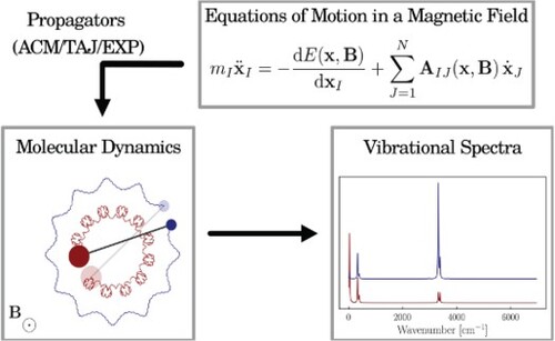
Ab initio molecular dynamics in a magnetic field requires solving equations of motion with velocity-dependent forces – namely, the Lorentz force arising from the nuclear charges moving in a magnetic field and the Berry force arising from the shielding of these charges from the magnetic field by the surrounding electrons. In this work, we revisit two existing propagators for these equations of motion, the auxiliary-coordinates-and-momenta (ACM) propagator and the Tajima propagator (TAJ), and compare them with a new exponential (EXP) propagator based on the Magnus expansion. Additionally, we explore limits (for example, the zero-shielding limit), the implementation of higher-order integration schemes, and series truncation to reduce computational cost by carrying out simulations of a HeH${}^{+}$ model system for a wide range of field strengths. While being as efficient as the TAJ propagator, the EXP propagator is the only propagator that converges to both the schemes of Spreiter and Walter (derived for systems without shielding of the Lorentz force) and to the exact cyclotronic motion of a charged particle. Since it also performs best in our model simulations, we conclude that the EXP propagator is the recommended propagator for molecules in magnetic fields.

GRAPHICAL ABSTRACT

KEYWORDS:

• Molecular dynamics
• magnetic field
• Berry curvature
• time propagation
• Magnus expansion

1. Introduction

Since the first simulations more than 50 years ago [1,2], molecular dynamics has become a ubiquitous tool in computational chemistry, allowing for the calculation of reaction rates and energies [3], the exploration of reaction networks [4,5], and the prediction of vibrational spectra [6–9], including infrared, Raman, and circular dichroism spectroscopies. The principal idea is to solve the equations of motion (1) $\begin{array}{r}{m}_I{\ddot{\mathbf{x}}}_I=-{\displaystyle \frac{\mathrm{d}E\left(\mathbf{x}\right)}{\mathrm{d}{\mathbf{x}}_I}},\mathbf{x}=\left(\begin{array}{c}{\mathbf{x}}_1\\ ⋮\\ {\mathbf{x}}_N\end{array}\right),\end{array}$(1) to determine the motion of a set of N nuclei with masses $m_1,\dots m_N$ and positions ${\mathbf{x}}_1\left(t\right),\dots {\mathbf{x}}_N\left(t\right)$. The potential $E\left(\mathbf{x}\right)$ and the corresponding gradient are usually determined using force-field or (for smaller systems) ab initio methods, while the equations of motion are solved using propagators such as the velocity Verlet algorithm [10,11] or higher-order schemes [12,13].

In a magnetic field $\mathbf{B}$, a classical particle of charge $q_I$ experiences an additional Lorentz force: (2) $\begin{array}{r}{m}_I{\ddot{\mathbf{x}}}_I=-{\displaystyle \frac{\mathrm{d}E\left(\mathbf{x}\right)}{\mathrm{d}{\mathbf{x}}_I}}-q_I\mathbf{B}\times {\dot{\mathbf{x}}}_I.\end{array}$(2) More than 20 years ago, Spreiter and Walter recognised that the appearance of this velocity-dependent force requires a modification of the velocity Verlet scheme [14]. Their algorithm, which relies on a Taylor expansion, has been incorporated into well-known software packages [15,16] and has been employed in diverse applications [17–19].

Taking into account the electrons as quantum particles within the Born–Oppenheimer approximation, the energy becomes dependent on the magnetic field [20–26], while the velocity-dependent force assumes a more general form [27–29]: (3) $\begin{array}{r}{m}_I{\ddot{\mathbf{x}}}_I=-{\displaystyle \frac{\mathrm{d}E(\mathbf{x},\mathbf{B})}{\mathrm{d}{\mathbf{x}}_I}}+\sum _{J=1}^N{\mathbf{A}}_{\mathrm{IJ}}(\mathbf{x},\mathbf{B}){\dot{\mathbf{x}}}_J.\end{array}$(3) Here, the last term contains not only the bare Lorentz force acting on the nuclei [see Equation (2(2) $\begin{array}{r}{m}_I{\ddot{\mathbf{x}}}_I=-{\displaystyle \frac{\mathrm{d}E\left(\mathbf{x}\right)}{\mathrm{d}{\mathbf{x}}_I}}-q_I\mathbf{B}\times {\dot{\mathbf{x}}}_I.\end{array}$(2) )], but also a contribution from the Berry curvature [30,31], reflecting the shielding of the nuclei by the electrons [32,33] and introducing a coupling between the motion of different nuclei [34,35].

While the form and the implications of Equation (3(3) $\begin{array}{r}{m}_I{\ddot{\mathbf{x}}}_I=-{\displaystyle \frac{\mathrm{d}E(\mathbf{x},\mathbf{B})}{\mathrm{d}{\mathbf{x}}_I}}+\sum _{J=1}^N{\mathbf{A}}_{\mathrm{IJ}}(\mathbf{x},\mathbf{B}){\dot{\mathbf{x}}}_J.\end{array}$(3) ) were discussed more than three decades ago [27,36,37], there are only a few examples where it has been actually solved for a molecular system in a magnetic field. Ceresoli and coworkers simulated an H${}_2$ model system in 2007, integrating the equations of motion with a Runge–Kutta scheme [28]. In 2021, Peters and coworkers were the first to conduct accurate dynamics of H${}_2$ using the auxiliary-coordinates-and-momenta (ACM) propagator [29], which is derived from a general scheme for propagating nonseparable Hamiltonians by Tao [38]. A more extensive study was conducted by Monzel and coworkers [39] in 2022, studying H${}_2$ and LiH with the Tajima (TAJ) propagator, originating from particle physics [40].

In this work, we introduce a new propagator that we refer to as the exponential (EXP) propagator. It is inspired by the fact that equations of type (4) $\begin{array}{r}\dot{\mathbf{c}}\left(t\right)=-\mathrm{i}\mathbf{H}\left(t\right)\mathbf{c}\left(t\right),\mathbf{c}\left(t_0\right)={\mathbf{c}}_0,\end{array}$(4) can, for a sufficiently small time interval $[t_0,t]$, be solved exactly using the Magnus expansion [41] and approximated using matrix exponential(s) of $-\mathrm{i}\mathbf{H}$ [42]. Such equations appear, for example, in time propagations in time-dependent Kohn–Sham theory [43] and in surface-hopping algorithms [44], where $\mathbf{c}$ corresponds to a vector of state amplitudes, while $\mathbf{H}$ is the Hamiltonian matrix containing energies of and couplings between the states. Here, we compare the EXP propagator to the previously published ACM and TAJ propagators, regarding their theoretical foundation, their time-step requirements, their performance during actual simulations, and properties, such as their behaviour in the zero-field case [see Equation (1(1) $\begin{array}{r}{m}_I{\ddot{\mathbf{x}}}_I=-{\displaystyle \frac{\mathrm{d}E\left(\mathbf{x}\right)}{\mathrm{d}{\mathbf{x}}_I}},\mathbf{x}=\left(\begin{array}{c}{\mathbf{x}}_1\\ ⋮\\ {\mathbf{x}}_N\end{array}\right),\end{array}$(1) )], in the zero-shielding case [see Equation (2(2) $\begin{array}{r}{m}_I{\ddot{\mathbf{x}}}_I=-{\displaystyle \frac{\mathrm{d}E\left(\mathbf{x}\right)}{\mathrm{d}{\mathbf{x}}_I}}-q_I\mathbf{B}\times {\dot{\mathbf{x}}}_I.\end{array}$(2) )], and in the cyclotron limit [only the Lorentz force in Equation (2(2) $\begin{array}{r}{m}_I{\ddot{\mathbf{x}}}_I=-{\displaystyle \frac{\mathrm{d}E\left(\mathbf{x}\right)}{\mathrm{d}{\mathbf{x}}_I}}-q_I\mathbf{B}\times {\dot{\mathbf{x}}}_I.\end{array}$(2) )]. We use simulations of a HeH${}^{+}$ model system to corroborate our theoretical findings and test schemes to further reduce the computational cost.

Having established the equations of motion, their propagation, and the weak-field limit for the step size in Sections 2.1–2.3, respectively, we derive the working equations of propagators in the absence of a field as well as the ACM, TAJ, and EXP propagators in Sections 2.4–2.7 and compare them in Section 2.8. Computational details for the HeH${}^{+}$ simulations are given in Section 3, while the results of these simulations are presented and discussed in Section 4. Conclusions and an outlook are given in Section 5.

2. Theory

2.1. Equations of motion

Within the Born–Oppenheimer approximation, the equations of motion of a molecule in a magnetic field are given by [27–29] (5) $\begin{array}{r}{M}_I{\ddot{\mathbf{R}}}_I=-{\displaystyle \frac{\mathrm{\partial }E({\mathbf{R}}_{},\mathbf{B})}{\mathrm{\partial }{\mathbf{R}}_I}}+\sum _{J=1}^{N_{\mathrm{nuc}}}\left[{\mathbf{\Omega }}_{\mathrm{IJ}}\right({\mathbf{R}}_{},\mathbf{B})-{\delta }_{\mathrm{IJ}}{Z}_I\tilde{\mathbf{B}}]{\dot{\mathbf{R}}}_J.\end{array}$(5) Here, we use indices $I,J,\dots$ for the $N_{\mathrm{nuc}}$ nuclei. ${\mathbf{R}}_I$, $Z_I$, $M_I$, and ${\dot{\mathbf{R}}}_I$ are the position, charge, mass, and velocity of nucleus I, while the $3N_{\mathrm{nuc}}$-dimensional column vector ${\mathbf{R}}_{}$ denotes the collective nuclear coordinates: (6) $\begin{array}{r}{\mathbf{R}}_{}=\left(\begin{array}{c}{\mathbf{R}}_1\\ ⋮\\ {\mathbf{R}}_{N_{\mathrm{nuc}}}\end{array}\right),{\mathbf{R}}_I=\left(\begin{array}{c}{R}_{I\mathrm{x}}\\ R_{I\mathrm{y}}\\ R_{I\mathrm{z}}\end{array}\right)\end{array}$(6) We represent the uniform magnetic field $\mathbf{B}$ of strength B by the $3\times 3$ antisymmetric matrix $\tilde{\mathbf{B}}$ in the manner (7) $\begin{array}{r}\tilde{\mathbf{B}}=\left(\begin{array}{ccc}0& -B_{\mathrm{z}}& B_{\mathrm{y}}\\ B_{\mathrm{z}}& 0& -B_{\mathrm{x}}\\ -B_{\mathrm{y}}& B_{\mathrm{x}}& 0\end{array}\right),\mathbf{B}=\left(\begin{array}{c}{B}_{\mathrm{x}}\\ B_{\mathrm{y}}\\ B_{\mathrm{z}}\end{array}\right),B=|\mathbf{B}|\end{array}$(7) so that (8) $\begin{array}{r}\tilde{\mathbf{B}}{\dot{\mathbf{R}}}_I=\mathbf{B}\times {\dot{\mathbf{R}}}_I.\end{array}$(8) The first term in Equation (5(5) $\begin{array}{r}{M}_I{\ddot{\mathbf{R}}}_I=-{\displaystyle \frac{\mathrm{\partial }E({\mathbf{R}}_{},\mathbf{B})}{\mathrm{\partial }{\mathbf{R}}_I}}+\sum _{J=1}^{N_{\mathrm{nuc}}}\left[{\mathbf{\Omega }}_{\mathrm{IJ}}\right({\mathbf{R}}_{},\mathbf{B})-{\delta }_{\mathrm{IJ}}{Z}_I\tilde{\mathbf{B}}]{\dot{\mathbf{R}}}_J.\end{array}$(5) ) is the gradient of the Born–Oppenheimer electronic energy, obtained at some ab initio level of theory, (9) $\begin{array}{r}E({\mathbf{R}}_{},\mathbf{B})=〈{\varphi }_{}({\mathbf{R}}_{},\mathbf{B})|H_{\mathrm{el}}({\mathbf{R}}_{},\mathbf{B})|{\varphi }_{}({\mathbf{R}}_{},\mathbf{B})〉,\end{array}$(9) where $H_{\mathrm{el}}^{}({\mathbf{r}}_{},{\mathbf{R}}_{},\mathbf{B})$ and ${\varphi }_{}({\mathbf{r}}_{};{\mathbf{R}}_{},\mathbf{B})$ are the electronic Hamiltonian and wave function, respectively, both of which depend on the electronic coordinates $\mathbf{r}$ [over which the integration is performed in Equation (9(9) $\begin{array}{r}E({\mathbf{R}}_{},\mathbf{B})=〈{\varphi }_{}({\mathbf{R}}_{},\mathbf{B})|H_{\mathrm{el}}({\mathbf{R}}_{},\mathbf{B})|{\varphi }_{}({\mathbf{R}}_{},\mathbf{B})〉,\end{array}$(9) )]. The second term in Equation (5(5) $\begin{array}{r}{M}_I{\ddot{\mathbf{R}}}_I=-{\displaystyle \frac{\mathrm{\partial }E({\mathbf{R}}_{},\mathbf{B})}{\mathrm{\partial }{\mathbf{R}}_I}}+\sum _{J=1}^{N_{\mathrm{nuc}}}\left[{\mathbf{\Omega }}_{\mathrm{IJ}}\right({\mathbf{R}}_{},\mathbf{B})-{\delta }_{\mathrm{IJ}}{Z}_I\tilde{\mathbf{B}}]{\dot{\mathbf{R}}}_J.\end{array}$(5) ) is the Lorentz force arising from the nuclear charge screened by the surrounding electrons. This shielding is represented by the Berry curvature, whose IJ blocks, (10) $\begin{array}{r}{\mathbf{\Omega }}_{\mathrm{IJ}}({\mathbf{R}}_{},\mathbf{B})=\left(\begin{array}{ccc}{\mathrm{\Omega }}_{I\mathrm{x}J\mathrm{x}}({\mathbf{R}}_{},\mathbf{B})& {\mathrm{\Omega }}_{I\mathrm{x}J\mathrm{y}}({\mathbf{R}}_{},\mathbf{B})& {\mathrm{\Omega }}_{I\mathrm{x}J\mathrm{z}}({\mathbf{R}}_{},\mathbf{B})\\ {\mathrm{\Omega }}_{I\mathrm{y}J\mathrm{x}}({\mathbf{R}}_{},\mathbf{B})& {\mathrm{\Omega }}_{I\mathrm{y}J\mathrm{y}}({\mathbf{R}}_{},\mathbf{B})& {\mathrm{\Omega }}_{I\mathrm{y}J\mathrm{z}}({\mathbf{R}}_{},\mathbf{B})\\ {\mathrm{\Omega }}_{I\mathrm{z}J\mathrm{x}}({\mathbf{R}}_{},\mathbf{B})& {\mathrm{\Omega }}_{I\mathrm{z}J\mathrm{y}}({\mathbf{R}}_{},\mathbf{B})& {\mathrm{\Omega }}_{I\mathrm{z}J\mathrm{z}}({\mathbf{R}}_{},\mathbf{B})\end{array}\right),\end{array}$(10) are Cartesian matrices whose elements (here we only show the xy-element), (11) $\begin{array}{r}{\mathrm{\Omega }}_{I\mathrm{x}J\mathrm{y}}({\mathbf{R}}_{},\mathbf{B})=-2\hslash \mathrm{\Im }〈{\displaystyle \frac{\mathrm{\partial }{\varphi }_{}({\mathbf{R}}_{},\mathbf{B})}{\mathrm{\partial }{R}_{I\mathrm{x}}}}|{\displaystyle \frac{\mathrm{\partial }{\varphi }_{}({\mathbf{R}}_{},\mathbf{B})}{\mathrm{\partial }{R}_{J\mathrm{y}}}}〉,\end{array}$(11) are determined from derivatives of the electronic wave function with respect to the corresponding nuclear coordinates. For more details on the calculation (at the Hartree–Fock level of theory) and interpretation of the Berry curvature, see Refs. [30–33].

With $\mathbf{M}$ being the $3N_{\mathrm{nuc}}\times 3N_{\mathrm{nuc}}$-dimensional matrix with the nuclear masses $M_I$ on the diagonal, we can define the kinetic momenta of the nuclei as (12) $\begin{array}{r}{\mathbf{\Pi }}_{}=\mathbf{M}{\dot{\mathbf{R}}}_{}.\end{array}$(12) We may now rewrite the nuclear equations of motion in Equation (5(5) $\begin{array}{r}{M}_I{\ddot{\mathbf{R}}}_I=-{\displaystyle \frac{\mathrm{\partial }E({\mathbf{R}}_{},\mathbf{B})}{\mathrm{\partial }{\mathbf{R}}_I}}+\sum _{J=1}^{N_{\mathrm{nuc}}}\left[{\mathbf{\Omega }}_{\mathrm{IJ}}\right({\mathbf{R}}_{},\mathbf{B})-{\delta }_{\mathrm{IJ}}{Z}_I\tilde{\mathbf{B}}]{\dot{\mathbf{R}}}_J.\end{array}$(5) ) in the more convenient form (13) $\begin{array}{r}{\dot{\mathbf{\Pi }}}_{}={\mathbf{F}}_{}^{}({\mathbf{R}}_{},\mathbf{B})+{\mathbf{W}}_{}({\mathbf{R}}_{},\mathbf{B}){\mathbf{\Pi }}_{},\end{array}$(13) where ${\mathbf{F}}_{}^{}({\mathbf{R}}_{},\mathbf{B})$ is the $3N_{\mathrm{nuc}}$-dimensional vector of the Born–Oppenheimer gradient forces and ${\mathbf{W}}_{}({\mathbf{R}}_{},\mathbf{B})$ is a $3N_{\mathrm{nuc}}\times 3N_{\mathrm{nuc}}$ matrix, whose IJ blocks of dimension $3\times 3$ contain the corresponding block of the Berry curvature as well as the contribution from the bare (unscreened) Lorentz force: (14) $\begin{array}{r}{\mathbf{W}}_{\mathrm{IJ}}({\mathbf{R}}_{},\mathbf{B})=M_J^{-1}\left[{\mathbf{\Omega }}_{\mathrm{IJ}}\right({\mathbf{R}}_{},\mathbf{B})-{\delta }_{\mathrm{IJ}}{Z}_I\tilde{\mathbf{B}}].\end{array}$(14) The form of the equations of motion given in Equation (13(13) $\begin{array}{r}{\dot{\mathbf{\Pi }}}_{}={\mathbf{F}}_{}^{}({\mathbf{R}}_{},\mathbf{B})+{\mathbf{W}}_{}({\mathbf{R}}_{},\mathbf{B}){\mathbf{\Pi }}_{},\end{array}$(13) ) highlights that the effect of the magnetic field is twofold: It changes the potential energy surface leading to different Born–Oppenheimer gradient forces and it introduces an additional, velocity-dependent term.

2.2. Propagators: general considerations

The main objective of this theory section is to discuss how these modified equations of motion can be integrated efficiently using different propagators. We denote by (15) $\begin{array}{rl}{\mathbf{x}}_a& ={\mathbf{R}}_{}(t+a_{}\mathrm{\Delta t}),\end{array}$(15) (16) $\begin{array}{rl}{\mathit{\pi }}_a& =\mathbf{M}{\dot{\mathbf{R}}}_{}(t+a_{}\mathrm{\Delta t}),\end{array}$(16) the position and momentum, respectively, of the system at time $a_{}$ relative to time $t$ in units of the time step $\mathrm{\Delta t}$. Introducing the notation (17) $\begin{array}{rl}{\mathbf{f}}_a& ={\mathbf{F}}_{}^{}({\mathbf{x}}_a,\mathbf{B}),\end{array}$(17) (18) $\begin{array}{rl}{\mathbf{w}}_a& ={\mathbf{W}}_{}({\mathbf{x}}_a,\mathbf{B}),\end{array}$(18) we may now express the equations of motion in terms of differentials with respect to the factor $a_{}$ (19) $\begin{array}{rl}{\dot{\mathit{\pi }}}_a& =\mathrm{\Delta t}{}^{-1}{\displaystyle \frac{\mathrm{\partial }{\mathit{\pi }}_a}{\mathrm{\partial }{a}_{}}}={\mathbf{f}}_a+{\mathbf{w}}_a{\mathit{\pi }}_a,\end{array}$(19) (20) $\begin{array}{rl}{\dot{\mathbf{x}}}_a& =\mathrm{\Delta t}{}^{-1}{\displaystyle \frac{\mathrm{\partial }{\mathbf{x}}_a}{\mathrm{\partial }a}}={\mathbf{M}}^{-1}{\mathit{\pi }}_a.\end{array}$(20) The choice of the step length $\mathrm{\Delta t}$, here appearing as a prefactor, will be discussed in the next subsection.

In this notation, a propagator is defined as a scheme that updates the coordinates (${\mathbf{x}}_0\to {\mathbf{x}}_1$) and momenta (${\mathit{\pi }}_0\to {\mathit{\pi }}_1$) for a given $\mathrm{\Delta t}$. Since Equations (19(19) $\begin{array}{rl}{\dot{\mathit{\pi }}}_a& =\mathrm{\Delta t}{}^{-1}{\displaystyle \frac{\mathrm{\partial }{\mathit{\pi }}_a}{\mathrm{\partial }{a}_{}}}={\mathbf{f}}_a+{\mathbf{w}}_a{\mathit{\pi }}_a,\end{array}$(19) ) and (20(20) $\begin{array}{rl}{\dot{\mathbf{x}}}_a& =\mathrm{\Delta t}{}^{-1}{\displaystyle \frac{\mathrm{\partial }{\mathbf{x}}_a}{\mathrm{\partial }a}}={\mathbf{M}}^{-1}{\mathit{\pi }}_a.\end{array}$(20) ) depend on each other, they are usually solved alternately for a series of substeps. To ease their reading, we will only derive working equations for a single set of those substeps, (21) $\begin{array}{rl}{\mathit{\pi }}_0\to {\mathit{\pi }}_a:{\mathit{\pi }}_a& =\mathrm{\Delta t}{\int }_0^{a_{}}({\mathbf{f}}_{\alpha }+{\mathbf{w}}_{\alpha }{\mathit{\pi }}_{\alpha })\mathrm{d}\alpha +{\mathit{\pi }}_0,\end{array}$(21) (22) $\begin{array}{rl}{\mathbf{x}}_0\to {\mathbf{x}}_{b_{}}:{\mathbf{x}}_{b_{}}& =\mathrm{\Delta t}{\mathbf{M}}^{-1}{\int }_0^{b_{}}{\mathit{\pi }}_{\text{β}}\mathrm{d}\text{β}+{\mathbf{x}}_0,\end{array}$(22) where ${\mathbf{x}}_0$ and ${\mathit{\pi }}_0$ are initial values and $a_{}$ and $b_{}$ are arbitrary step lengths in units of $\mathrm{\Delta t}$. Equations for all other substeps can then be derived by adjusting the initial values and step lengths accordingly.

To evaluate the integrals in Equations (21(21) $\begin{array}{rl}{\mathit{\pi }}_0\to {\mathit{\pi }}_a:{\mathit{\pi }}_a& =\mathrm{\Delta t}{\int }_0^{a_{}}({\mathbf{f}}_{\alpha }+{\mathbf{w}}_{\alpha }{\mathit{\pi }}_{\alpha })\mathrm{d}\alpha +{\mathit{\pi }}_0,\end{array}$(21) ) and (22(22) $\begin{array}{rl}{\mathbf{x}}_0\to {\mathbf{x}}_{b_{}}:{\mathbf{x}}_{b_{}}& =\mathrm{\Delta t}{\mathbf{M}}^{-1}{\int }_0^{b_{}}{\mathit{\pi }}_{\text{β}}\mathrm{d}\text{β}+{\mathbf{x}}_0,\end{array}$(22) ), we will draw inspiration from the mean-value theorems. They state that, for real-valued functions $\phi \left(\alpha \right)$ and $\psi \left(\alpha \right)$ that are continuous in $[0,a]$, there exists a point $0\le b\le a$ such that (23) $\begin{array}{r}{\int }_0^a\phi \left(\alpha \right)\mathrm{d}\alpha =\mathrm{a\phi }\left(b\right),\end{array}$(23) and (24) $\begin{array}{rl}{\int }_0^a\phi \left(\alpha \right)\psi \left(\alpha \right)\mathrm{d}t& =\psi \left(0\right){\int }_0^b\phi \left(\alpha \right)\mathrm{d}\alpha \\ & +\psi \left(a\right){\int }_b^a\phi \left(\alpha \right)\mathrm{d}\alpha .\end{array}$(24) The corresponding statements are not guaranteed to hold for vector-valued functions; however, we will at one point rely on them as approximations. Specifically, we use the forms (25) $\begin{array}{r}{\int }_0^{a_{}}\mathit{\phi }\left(\alpha \right)\mathrm{d}\alpha \approx \mathit{\phi }\left(b_{}\right){\int }_0^{a_{}}\mathrm{d}\alpha =a_{}\mathit{\phi }\left(b_{}\right),\end{array}$(25) and (26) $\begin{array}{rl}{\int }_0^{a_{}}\mathit{\psi }\left(\alpha \right)\mathit{\phi }\left(\alpha \right)\mathrm{d}\alpha & \approx {\int }_0^{b_{}}\mathit{\psi }\left(\alpha \right)\mathit{\phi }\left(0\right)\mathrm{d}\alpha \\ & +{\int }_{b_{}}^{a_{}}\mathit{\psi }\left(\alpha \right)\mathit{\phi }\left(a_{}\right)\mathrm{d}\alpha ,\end{array}$(26) to approximate integrals over two vectors of continuous functions $\mathit{\phi }\left(\alpha \right)$ and $\mathit{\psi }\left(\alpha \right)$. Note that both the midpoint rule and the trapezoidal rule can be derived from these mean-value approximations by choosing $b_{}=a_{}/2$ and, in case of latter, $\mathit{\psi }\left(\alpha \right)=\mathbf{1}$: (27) $\begin{array}{rl}{\int }_0^{a_{}}\mathit{\phi }\left(\alpha \right)\mathrm{d}\alpha & \approx \mathit{\phi }\left(a_{}/2\right){\int }_0^{a_{}}\mathrm{d}\alpha =a_{}\mathit{\phi }\left(a_{}/2\right)\end{array}$(27) (28) $\begin{array}{rl}{\int }_0^{a_{}}\mathit{\phi }\left(\alpha \right)\mathrm{d}\alpha & \approx {\int }_0^{a_{}/2}\mathit{\phi }\left(0\right)\mathrm{d}\alpha \\ & +{\int }_{a_{}/2}^{a_{}}\mathit{\phi }\left(1\right)\mathrm{d}\alpha ={\displaystyle \frac{a_{}}{2}}\left[\mathit{\phi }\right(0)+\mathit{\phi }(1\left)\right]\end{array}$(28)

2.3. Choice of step size

The error introduced by a given propagator depends on the applied step size $\mathrm{\Delta t}$. Before considering the different propagators, we discuss briefly in this subsection the restriction on the time step imposed by an external magnetic field. As in field-free simulations, we demand that the time step $\mathrm{\Delta t}$ is significantly smaller than the fastest molecular vibration. In addition, we demand that the matrix $\mathrm{\Delta t}{\mathbf{w}}_a$ is convergent for all a, meaning that (29) $\begin{array}{r}\underset{n\to \mathrm{\infty }}{lim}{\left[\mathrm{\Delta }t{\mathbf{w}}_a\right]}^n=\mathbf{0}\end{array}$(29) Introducing the spectral radius ρ (30) $\begin{array}{r}\sqrt{\rho \left({\mathbf{w}}_a^{\mathrm{T}}{\mathbf{w}}_a\right)}={\omega }_a,\end{array}$(30) which we loosely interpret as a cyclotron frequency, we have (31) $\begin{array}{rl}& \underset{n\to \mathrm{\infty }}{lim}\Vert {\left[\mathrm{\Delta }t{\mathbf{w}}_a\right]}^n\Vert \\ & \propto \underset{n\to \mathrm{\infty }}{lim}\mathrm{\Delta t}{}^n\rho {\left({\mathbf{w}}_a^{\mathrm{T}}{\mathbf{w}}_a\right)}^{n/2}=\underset{n\to \mathrm{\infty }}{lim}(\mathrm{\Delta t}{\omega }_a{)}^n\end{array}$(31) in some matrix norm $\Vert \cdot \Vert$. Consequently, Equation (29(29) $\begin{array}{r}\underset{n\to \mathrm{\infty }}{lim}{\left[\mathrm{\Delta }t{\mathbf{w}}_a\right]}^n=\mathbf{0}\end{array}$(29) ) holds when (32) $\begin{array}{r}\mathrm{\Delta t}<{\omega }_a^{-1}.\end{array}$(32) This weak-field limit, as defined by Spreiter and Walter [14], means that the time step is small enough to resolve the cyclotronic motion. For a neutral molecule, the charge–mass ratio is roughly on the order of ${10}^{-4}$a.u., so that (33) $\begin{array}{r}{\omega }_a\sim {10}^{-4}B.\end{array}$(33) Time steps of up to 100 a.u. (2.4 fs) therefore allow for simulations in field strengths up to about $10{\mathrm{B}}_0$, covering the entire range of field strengths from the (particularly interesting) intermediate regime ($<1{\mathrm{B}}_0$) up to the Landau regime.

2.4. Propagators in the absence of a field

For the field-free case, ${\mathbf{w}}_{}$ is zero so that we can directly apply the mean-value approximation Equation (25(25) $\begin{array}{r}{\int }_0^{a_{}}\mathit{\phi }\left(\alpha \right)\mathrm{d}\alpha \approx \mathit{\phi }\left(b_{}\right){\int }_0^{a_{}}\mathrm{d}\alpha =a_{}\mathit{\phi }\left(b_{}\right),\end{array}$(25) ) to Equations (21(21) $\begin{array}{rl}{\mathit{\pi }}_0\to {\mathit{\pi }}_a:{\mathit{\pi }}_a& =\mathrm{\Delta t}{\int }_0^{a_{}}({\mathbf{f}}_{\alpha }+{\mathbf{w}}_{\alpha }{\mathit{\pi }}_{\alpha })\mathrm{d}\alpha +{\mathit{\pi }}_0,\end{array}$(21) ) and (22(22) $\begin{array}{rl}{\mathbf{x}}_0\to {\mathbf{x}}_{b_{}}:{\mathbf{x}}_{b_{}}& =\mathrm{\Delta t}{\mathbf{M}}^{-1}{\int }_0^{b_{}}{\mathit{\pi }}_{\text{β}}\mathrm{d}\text{β}+{\mathbf{x}}_0,\end{array}$(22) ): (34) $\begin{array}{rl}{\mathit{\pi }}_a& =\mathrm{\Delta t}{\int }_0^{a_{}}{\mathbf{f}}_{\alpha }\mathrm{d}\alpha +{\mathit{\pi }}_0\approx a_{}\mathrm{\Delta t}{\mathbf{f}}_{b_{}}+{\mathit{\pi }}_0\end{array}$(34) (35) $\begin{array}{rl}{\mathbf{x}}_{b_{}}& =\mathrm{\Delta t}{\mathbf{M}}^{-1}{\int }_0^{b_{}}{\mathit{\pi }}_{\text{β}}\mathrm{d}\text{β}+{\mathbf{x}}_0\approx b_{}\mathrm{\Delta t}{\mathbf{M}}^{-1}{\mathit{\pi }}_a+{\mathbf{x}}_0\end{array}$(35) As shown in Algorithm 1, both equations are solved alternately using the current forces and momenta as mean values to propagate the momenta and positions, respectively. The remaining task is now to come up with a series of $a_{}$'s and $b_{}$'s (denoted by the vectors $\mathbf{a}$ and $\mathbf{b}$) to approximate the mean values. The lengths of $\mathbf{a}$ and $\mathbf{b}$ (K + 1 and K) reflect the order K of the scheme.

In the standard velocity Verlet scheme (K = 1) [10,11], we set $\mathbf{a}=[0.5,0.5]$ and $\mathbf{b}=\left[1.0\right]$, so that we obtain: (36) $\begin{array}{rl}{\mathit{\pi }}_{0.5}^{\mathrm{VV}}& =0.5\mathrm{\Delta t}{\mathbf{f}}_0+{\mathit{\pi }}_0\end{array}$(36) (37) $\begin{array}{rl}{\mathbf{x}}_1^{\mathrm{VV}}& =\mathrm{\Delta t}\left[{\mathbf{M}}^{-1}{\mathit{\pi }}_{0.5}^{\mathrm{VV}}\right]+{\mathbf{x}}_0\end{array}$(37) (38) $\begin{array}{rl}{\mathit{\pi }}_1^{\mathrm{VV}}& =0.5\mathrm{\Delta t}{\mathbf{f}}_1+{\mathit{\pi }}_{0.5}^{\mathrm{VV}}\end{array}$(38) Note that this quadrature corresponds to solving the full integral ($a_{}=1$) in Equation (34(34) $\begin{array}{rl}{\mathit{\pi }}_a& =\mathrm{\Delta t}{\int }_0^{a_{}}{\mathbf{f}}_{\alpha }\mathrm{d}\alpha +{\mathit{\pi }}_0\approx a_{}\mathrm{\Delta t}{\mathbf{f}}_{b_{}}+{\mathit{\pi }}_0\end{array}$(34) ) with the trapezoidal [see Equation (28(28) $\begin{array}{rl}{\int }_0^{a_{}}\mathit{\phi }\left(\alpha \right)\mathrm{d}\alpha & \approx {\int }_0^{a_{}/2}\mathit{\phi }\left(0\right)\mathrm{d}\alpha \\ & +{\int }_{a_{}/2}^{a_{}}\mathit{\phi }\left(1\right)\mathrm{d}\alpha ={\displaystyle \frac{a_{}}{2}}\left[\mathit{\phi }\right(0)+\mathit{\phi }(1\left)\right]\end{array}$(28) )] and the full integral in Equation (35(35) $\begin{array}{rl}{\mathbf{x}}_{b_{}}& =\mathrm{\Delta t}{\mathbf{M}}^{-1}{\int }_0^{b_{}}{\mathit{\pi }}_{\text{β}}\mathrm{d}\text{β}+{\mathbf{x}}_0\approx b_{}\mathrm{\Delta t}{\mathbf{M}}^{-1}{\mathit{\pi }}_a+{\mathbf{x}}_0\end{array}$(35) ) ($b_{}=1$) with the midpoint rule [see Equation (27(27) $\begin{array}{rl}{\int }_0^{a_{}}\mathit{\phi }\left(\alpha \right)\mathrm{d}\alpha & \approx \mathit{\phi }\left(a_{}/2\right){\int }_0^{a_{}}\mathrm{d}\alpha =a_{}\mathit{\phi }\left(a_{}/2\right)\end{array}$(27) )]. As a consequence of this the velocity Verlet algorithm is symplectic, time-reversible, and of second-order accuracy. However, it has been shown that higher-order schemes [12,13], can significantly increase the stability of the dynamics.

Unfortunately, there is no straightforward expansion of the upper scheme towards systems with velocity-dependent forces since, taking the velocity Verlet algorithm as an example, the step of Equation (38(38) $\begin{array}{rl}{\mathit{\pi }}_1^{\mathrm{VV}}& =0.5\mathrm{\Delta t}{\mathbf{f}}_1+{\mathit{\pi }}_{0.5}^{\mathrm{VV}}\end{array}$(38) ) becomes (39) $\begin{array}{r}{\mathit{\pi }}_1\approx 0.5\mathrm{\Delta t}({\mathbf{f}}_1+{\mathbf{w}}_1{\mathit{\pi }}_1)+{\mathit{\pi }}_{0.5}\end{array}$(39) The mismatch between the required (${\mathit{\pi }}_1$) and the available (${\mathit{\pi }}_{0.5}$) momenta for the propagation leads to a systematic error in the integration of the equations of motion [29]. Clearly, there is a need to develop alternative propagators, which will be done in the following subsections.

2.5. Auxiliary-coordinates-and-momenta propagator

The auxiliary-coordinates-and-momenta (ACM) propagator method was proposed by Tao for general nonseparable Hamiltonians [38] and adapted by Peters and coworkers for molecular simulations in a magnetic field [29]. The idea is to circumvent the mismatch in Equation (39(39) $\begin{array}{r}{\mathit{\pi }}_1\approx 0.5\mathrm{\Delta t}({\mathbf{f}}_1+{\mathbf{w}}_1{\mathit{\pi }}_1)+{\mathit{\pi }}_{0.5}\end{array}$(39) ), by introducing an additional pair of coordinates and momenta (${\mathbf{x}}_{}^{\prime },{\mathit{\pi }}_{}^{\prime }$) that are kept close to the original pair (${\mathbf{x}}_{},{\mathit{\pi }}_{}$) during the dynamics (${\mathbf{x}}_{}\approx {\mathbf{x}}_{}^{\prime }$ and ${\mathit{\pi }}_{}\approx {\mathit{\pi }}_{}^{\prime }$). If this coupling is sufficiently strong, we can write the propagation of ${\mathit{\pi }}_{}$ in terms of ${\mathit{\pi }}_{}^{\prime }$ and ${\mathbf{x}}_{}$ (40) $\begin{array}{rl}{\mathit{\pi }}_a& \approx a_{}\mathrm{\Delta t}[{\mathbf{f}}_{b_{}}+{\mathbf{w}}_{b_{}}{\mathit{\pi }}_{b_{}}^{\prime }]+{\mathit{\pi }}_0,\end{array}$(40) (41) $\begin{array}{rl}{\mathbf{x}}_{b_{}}& \approx b_{}\mathrm{\Delta t}\left[{\mathbf{M}}^{-1}{\mathit{\pi }}_a\right]+{\mathbf{x}}_0.\end{array}$(41) and the propagation of ${\mathit{\pi }}_{}^{\prime }$ in terms of ${\mathit{\pi }}_{}$ and ${\mathbf{x}}_{}^{\prime }$ (42) $\begin{array}{rl}{\mathit{\pi }}_{b_{}}^{\prime }& \approx b_{}\mathrm{\Delta t}[{\mathbf{f}}_a^{\prime }+{\mathbf{w}}_a^{\prime }{\mathit{\pi }}_a]+{\mathit{\pi }}_0^{\prime },\end{array}$(42) (43) $\begin{array}{rl}{\mathbf{x}}_a^{\prime }& \approx a_{}\mathrm{\Delta t}\left[{\mathbf{M}}^{-1}{\mathit{\pi }}_{b_{}}^{\prime }\right]+{\mathbf{x}}_0^{\prime },\end{array}$(43) The only remaining step is the coupling of coordinates and momenta, which is done when all quantities ${\mathbf{x}}_{}$, ${\mathit{\pi }}_{}$, ${\mathbf{x}}_{}^{\prime }$, and ${\mathit{\pi }}_{}^{\prime }$ are at the same time step by carrying out, for a given coupling constant s, the transformation [29] (44) $\begin{array}{r}\left(\begin{array}{c}{\mathbf{x}}_{c_{}}\\ {\mathbf{x}}_{c_{}}^{\prime }\\ {\mathbf{M}}^{-1}{\mathit{\pi }}_{c_{}}\\ {\mathbf{M}}^{-1}{\mathit{\pi }}_{c_{}}^{\prime }\end{array}\right)\to {\mathbf{s}}_{b_{}}^s\left(\begin{array}{c}{\mathbf{x}}_{c_{}}\\ {\mathbf{x}}_{c_{}}^{\prime }\\ {\mathbf{M}}^{-1}{\mathit{\pi }}_{c_{}}\\ {\mathbf{M}}^{-1}{\mathit{\pi }}_{c_{}}^{\prime }\end{array}\right)\end{array}$(44) with the coupling matrix (45) $\begin{array}{r}{\mathbf{s}}_{b_{}}^s={\displaystyle \frac{1}{2}}\left(\begin{array}{cccc}1+\cos \chi & 1-\cos \chi & s{}^{-1}\sin \chi & -s{}^{-1}\sin \chi \\ 1-\cos \chi & 1+\cos \chi & -s{}^{-1}\sin \chi & s{}^{-1}\sin \chi \\ s\sin \chi & -s\sin \chi & 1+\cos \chi & 1-\cos \chi \\ -s\sin \chi & s\sin \chi & 1-\cos \chi & 1+\cos \chi \end{array}\right)\end{array}$(45) where (46) $\begin{array}{r}\chi =s{b}_{}\mathrm{\Delta t}\end{array}$(46) Setting $s=0$ reduces the coupling matrix to the unity matrix, while setting it to $s=\pi /\left(c_{}\mathrm{\Delta t}\right)$ leads to a complete exchange of ${\mathbf{x}}_{}$ and ${\mathit{\pi }}_{}$ with ${\mathbf{x}}_{}^{\prime }$ and ${\mathit{\pi }}_{}^{\prime }$ and vice versa. The pseudo code for a general ACM propagator of order K is given in Algorithm 2.

2.6. Tajima propagator

An alternative to the ACM propagator is the Tajima (TAJ) propagator. Initially used in particle physics [40], it was rewritten for molecular applications by Monzel et al. [39]. Here, we present a slightly different derivation of the working equations that starts with applying the mean-value approximations [Equations (25(25) $\begin{array}{r}{\int }_0^{a_{}}\mathit{\phi }\left(\alpha \right)\mathrm{d}\alpha \approx \mathit{\phi }\left(b_{}\right){\int }_0^{a_{}}\mathrm{d}\alpha =a_{}\mathit{\phi }\left(b_{}\right),\end{array}$(25) ) and (26(26) $\begin{array}{rl}{\int }_0^{a_{}}\mathit{\psi }\left(\alpha \right)\mathit{\phi }\left(\alpha \right)\mathrm{d}\alpha & \approx {\int }_0^{b_{}}\mathit{\psi }\left(\alpha \right)\mathit{\phi }\left(0\right)\mathrm{d}\alpha \\ & +{\int }_{b_{}}^{a_{}}\mathit{\psi }\left(\alpha \right)\mathit{\phi }\left(a_{}\right)\mathrm{d}\alpha ,\end{array}$(26) )] to Equation (21(21) $\begin{array}{rl}{\mathit{\pi }}_0\to {\mathit{\pi }}_a:{\mathit{\pi }}_a& =\mathrm{\Delta t}{\int }_0^{a_{}}({\mathbf{f}}_{\alpha }+{\mathbf{w}}_{\alpha }{\mathit{\pi }}_{\alpha })\mathrm{d}\alpha +{\mathit{\pi }}_0,\end{array}$(21) ): (47) $\begin{array}{rl}{\mathit{\pi }}_a& \approx a_{}\mathrm{\Delta t}{\mathbf{f}}_{b_{}}+\mathrm{\Delta t}{\int }_0^{c_{}}{\mathbf{w}}_{\alpha }{\mathit{\pi }}_0\mathrm{d}\alpha \\ & +\mathrm{\Delta t}{\int }_{c_{}}^{a_{}}{\mathbf{w}}_{\alpha }{\mathit{\pi }}_a\mathrm{d}\alpha +{\mathit{\pi }}_0\end{array}$(47) Assuming that $c_{}=a_{}/2$ and that both integrals have the same mean value ${\mathbf{w}}_{b_{}}$, we obtain: (48) $\begin{array}{r}[\mathbf{1}-{\displaystyle \frac{a_{}}{2}}\mathrm{\Delta t}{\mathbf{w}}_{b_{}}]{\mathit{\pi }}_a\approx a_{}\mathrm{\Delta t}{\mathbf{f}}_b+[\mathbf{1}+{\displaystyle \frac{a_{}}{2}}\mathrm{\Delta t}{\mathbf{w}}_{b_{}}]{\mathit{\pi }}_0\end{array}$(48) Introducing the inverted matrix (49) $\begin{array}{r}{\mathbf{v}}_b^{c_{}}={[\mathbf{1}-c_{}\mathrm{\Delta }t{\mathbf{w}}_b]}^{-1},\end{array}$(49) we arrive at the working equation for the TAJ propagator, (50) $\begin{array}{r}{\mathit{\pi }}_a\approx {\mathbf{v}}_b^{a_{}/2}(a_{}\mathrm{\Delta t}{\mathbf{f}}_b+[\mathbf{1}+{\displaystyle \frac{a_{}}{2}}\mathrm{\Delta t}{\mathbf{w}}_b]{\mathit{\pi }}_0),\end{array}$(50) yielding the algorithm in Algorithm 3. In the weak-field limit [see Equation (29(29) $\begin{array}{r}\underset{n\to \mathrm{\infty }}{lim}{\left[\mathrm{\Delta }t{\mathbf{w}}_a\right]}^n=\mathbf{0}\end{array}$(29) )], we can expand the matrix inversion in a Neumann series: (51) $\begin{array}{r}{\mathbf{v}}_b^{c_{}}=\sum _{n=0}^{\mathrm{\infty }}{\left[c_{}\mathrm{\Delta }t{\mathbf{w}}_b\right]}^n=\sum _{n=0}^{N-1}{\left[c_{}\mathrm{\Delta }t{\mathbf{w}}_b\right]}^n+\mathcal{O}\left({\left[\mathrm{\Delta }t{\omega }_b\right]}^N\right)\end{array}$(51) In standard applications, we expect this series to converge fast. Using the estimate in Equation (33(33) $\begin{array}{r}{\omega }_a\sim {10}^{-4}B.\end{array}$(33) ) with B = 0.1 and $\mathrm{\Delta t}=10$ in atomic units, the error is on the order of ${10}^{-8}$ when using $N_{}=2$. Consequently, we can avoid the (comparably) high computational cost of matrix inversions during the simulations.

2.7. Exponential propagator

A general approach to solving first-order linear differential equations is the Magnus integrator method. Specifically, we may write (52) $\begin{array}{r}{\mathit{\pi }}_a=\mathrm{\Delta t}{\int }_{\gamma }^{a_{}}\exp \left({\mathbf{y}}_{\alpha ,a_{}}^{}\right){\mathbf{f}}_{\alpha }\mathrm{d}\alpha +\exp \left({\mathbf{y}}_{\gamma ,a_{}}^{}\right){\mathit{\pi }}_{\gamma }\end{array}$(52) where $\gamma$ is chosen so that the Magnus series [41], (53) $\begin{array}{rl}{\mathbf{y}}_{\gamma ,a_{}}^{}& =\mathrm{\Delta t}{\int }_{\gamma }^{a_{}}\mathrm{d}\alpha {\mathbf{w}}_{\alpha }\\ & +{\displaystyle \frac{1}{2}}(\mathrm{\Delta t}{)}^2{\int }_{\gamma }^{a_{}}\mathrm{d}\alpha {\int }_{\gamma }^{\alpha }\mathrm{d}\text{β}[{\mathbf{w}}_{\alpha },{\mathbf{w}}_{\text{β}}]+\cdots ,\end{array}$(53) converges. From ${\mathbf{y}}_{a_{},a_{}}^{}=\mathbf{0}$ and (54) $\begin{array}{r}\frac{\mathrm{\partial }\exp \left({\mathbf{y}}_{\gamma ,a_{}}\right)}{\mathrm{\partial }a}=\mathrm{\Delta t}{\mathbf{w}}_a\exp \left({\mathbf{y}}_{\gamma ,a_{}}^{}\right),\end{array}$(54) it is straightforward to verify that Equation (52(52) $\begin{array}{r}{\mathit{\pi }}_a=\mathrm{\Delta t}{\int }_{\gamma }^{a_{}}\exp \left({\mathbf{y}}_{\alpha ,a_{}}^{}\right){\mathbf{f}}_{\alpha }\mathrm{d}\alpha +\exp \left({\mathbf{y}}_{\gamma ,a_{}}^{}\right){\mathit{\pi }}_{\gamma }\end{array}$(52) ) solves Equation (19(19) $\begin{array}{rl}{\dot{\mathit{\pi }}}_a& =\mathrm{\Delta t}{}^{-1}{\displaystyle \frac{\mathrm{\partial }{\mathit{\pi }}_a}{\mathrm{\partial }{a}_{}}}={\mathbf{f}}_a+{\mathbf{w}}_a{\mathit{\pi }}_a,\end{array}$(19) ) and is thus an alternative to Equation (21(21) $\begin{array}{rl}{\mathit{\pi }}_0\to {\mathit{\pi }}_a:{\mathit{\pi }}_a& =\mathrm{\Delta t}{\int }_0^{a_{}}({\mathbf{f}}_{\alpha }+{\mathbf{w}}_{\alpha }{\mathit{\pi }}_{\alpha })\mathrm{d}\alpha +{\mathit{\pi }}_0,\end{array}$(21) ). We can set γ to zero from now on, since our choice of step size in Equation (32(32) $\begin{array}{r}\mathrm{\Delta t}<{\omega }_a^{-1}.\end{array}$(32) ) ensures the convergence of the Magnus series in this case. Truncating the Magnus series after the first term and applying the mean-value approximation [Equation (25(25) $\begin{array}{r}{\int }_0^{a_{}}\mathit{\phi }\left(\alpha \right)\mathrm{d}\alpha \approx \mathit{\phi }\left(b_{}\right){\int }_0^{a_{}}\mathrm{d}\alpha =a_{}\mathit{\phi }\left(b_{}\right),\end{array}$(25) )], the matrix exponential becomes (55) $\begin{array}{r}\exp \left({\mathbf{y}}_{\alpha ,a_{}}^{}\right)\approx \exp \left([a_{}-\alpha ]\mathrm{\Delta t}{\mathbf{w}}_{b_{}}\right)={\mathbf{u}}_{b_{}}^{a_{}-\alpha },\end{array}$(55) where we have introduced the matrix exponential (56) $\begin{array}{r}{\mathbf{u}}_{b_{}}^{}=\exp \left(\mathrm{\Delta t}{\mathbf{w}}_{b_{}}\right)\end{array}$(56) Equation (52(52) $\begin{array}{r}{\mathit{\pi }}_a=\mathrm{\Delta t}{\int }_{\gamma }^{a_{}}\exp \left({\mathbf{y}}_{\alpha ,a_{}}^{}\right){\mathbf{f}}_{\alpha }\mathrm{d}\alpha +\exp \left({\mathbf{y}}_{\gamma ,a_{}}^{}\right){\mathit{\pi }}_{\gamma }\end{array}$(52) ) now becomes: (57) $\begin{array}{r}{\mathit{\pi }}_a\approx \mathrm{\Delta t}{\int }_0^{a_{}}{\mathbf{u}}_{b_{}}^{a_{}-\alpha }\mathrm{d}\alpha {\mathbf{f}}_{b_{}}+{\mathbf{u}}_{b_{}}^{a_{}}{\mathit{\pi }}_0\end{array}$(57) Approximating the remaining integral via the midpoint rule [Equation (27(27) $\begin{array}{rl}{\int }_0^{a_{}}\mathit{\phi }\left(\alpha \right)\mathrm{d}\alpha & \approx \mathit{\phi }\left(a_{}/2\right){\int }_0^{a_{}}\mathrm{d}\alpha =a_{}\mathit{\phi }\left(a_{}/2\right)\end{array}$(27) )], we obtain (58) $\begin{array}{r}{\mathit{\pi }}_a\approx a_{}\mathrm{\Delta t}{\mathbf{u}}_{b_{}}^{a_{}/2}{\mathbf{f}}_{b_{}}+{\mathbf{u}}_{b_{}}^{a_{}}{\mathit{\pi }}_0={\mathbf{u}}_{b_{}}^{a_{}/2}[a_{}\mathrm{\Delta t}{\mathbf{f}}_{b_{}}+{\mathbf{u}}_{b_{}}^{a_{}/2}{\mathit{\pi }}_0]\end{array}$(58) as the exponential propagator (EXP) for the nuclear momenta in magnetic fields; see Algorithm 4. The matrix exponential can be expanded as (59) $\begin{array}{rl}{\mathbf{u}}_{b_{}}^{c_{}}& =\sum _{n=0}^{\mathrm{\infty }}{\displaystyle \frac{1}{n!}}{\left[c_{}\mathrm{\Delta }t{\mathbf{w}}_{b_{}}\right]}^n\\ & =\sum _{n=0}^{N-1}{\displaystyle \frac{1}{n!}}{\left[c_{}\mathrm{\Delta }t{\mathbf{w}}_{b_{}}\right]}^n+\mathcal{O}({\left[\mathrm{\Delta }t{\omega }_{}\right]}^N/N!).\end{array}$(59) In contrast to the Neumann series, this series converges unconditionally, for all step sizes.

2.8. Comparison of the propagators

We close this section by discussing a few properties of the introduced propagators. The results are summarised in Table 1. From Algorithms 2–4, we see that the ACM propagator is about three times more expensive than the other schemes, requiring $3K$ instead of K forces and Berry curvature calculations per step. In addition, it depends on the definition of a parameter ($s$), which has an influence on the stability of the dynamics. Moreover, unlike the ACM propagator, TAJ and EXP propagators converge to the correct zero-field solution when setting $\mathbf{B}$ and therefore ${\mathbf{w}}_b$ to zero.

Table 1. Comparison of the auxiliary coordinates and momenta (ACM), Tajima (TAJ), and exponential (EXP) propagator.

Criterion	ACM	TAJ	EXP
Forces calculations per step	$3K$	K	K
Parameter-free?	No	Yes	Yes
Correct zero-field limit?	No	Yes	Yes
Correct zero-shielding,	No	Yes	Yes
velocity Verlet limit?
Exact cyclotron limit?	No	No	Yes

As the correct zero-shielding limit, we define the propagators derived by Spreiter and Walter, which were constructed for the special case where the Berry curvature is zero. While their working equations clearly differ from the ACM propagator, we can compare them to the TAJ and EXP propagators by assuming a single particle with charge $Z_1$ and mass $M_1$, experiencing a time-dependent external force ${\mathbf{f}}_{}$ and a magnetic field of strength $B_{\mathrm{z}}$ in the z-direction. In this particular case, ${\mathbf{w}}_{}$ and thus ${\mathbf{u}}_{}^a$ and ${\mathbf{v}}_{}^a$ are constants (60) $\begin{array}{r}{\mathbf{w}}_{}=\left(\begin{array}{ccc}0& {\omega }_{}& 0\\ -{\omega }_{}& 0& 0\\ 0& 0& 0\end{array}\right){\omega }_{}={\displaystyle \frac{B_{\mathrm{z}}{Z}_1}{M_1}},\end{array}$(60) and the velocity Verlet variants of the EXP and TAJ propagator reduce to (61) $\begin{array}{rl}{\mathit{\pi }}_1^{\mathrm{EXP}}& ={\displaystyle \frac{\mathrm{\Delta }t}{2}}({\mathbf{u}}_{}^{0.25}{\mathbf{f}}_1+{\mathbf{u}}_{}^{0.75}{\mathbf{f}}_0)+{\mathbf{u}}_{}^1{\mathit{\pi }}_0,\end{array}$(61) (62) $\begin{array}{rl}{\mathit{\pi }}_1^{\mathrm{TAJ}}& ={\displaystyle \frac{\mathrm{\Delta }t}{2}}({\mathbf{v}}_{}^{0.25}{\mathbf{f}}_1+{\mathbf{v}}_{}^{0.25}[\mathbf{1}+{\displaystyle \frac{\mathrm{\Delta }t}{4}}{\mathbf{w}}_{}]{\mathbf{v}}_{}^{0.25}{\mathbf{f}}_0)\\ & +{\mathbf{v}}_{}^{0.25}[\mathbf{1}+{\displaystyle \frac{\mathrm{\Delta }t}{4}}{\mathbf{w}}_{}]{\mathbf{v}}_{}^{0.25}[\mathbf{1}+{\displaystyle \frac{\mathrm{\Delta }t}{4}}{\mathbf{w}}_{}]{\mathit{\pi }}_0,\end{array}$(62) respectively. Expanding ${\mathbf{u}}_{}^a$ and ${\mathbf{v}}_{}^a$ up to second order (63) $\begin{array}{rl}{\mathbf{u}}_{}^{a_{}}& =\mathbf{1}+a_{}\mathrm{\Delta t}{\mathbf{w}}_{}+{\displaystyle \frac{1}{2}}{a}_{}^2(\mathrm{\Delta t}{)}^2{\mathbf{w}}_{}^2+\mathcal{O}\left(\right[\mathrm{\Delta t}{]}^3)\end{array}$(63) (64) $\begin{array}{rl}{\mathbf{v}}_{}^{a_{}}& =\mathbf{1}+a_{}\mathrm{\Delta t}{\mathbf{w}}_{}+a_{}^2(\mathrm{\Delta t}{)}^2{\mathbf{w}}_{}^2+\mathcal{O}\left(\right[\mathrm{\Delta t}{]}^3)\end{array}$(64) and using the Taylor expansion of the forces in y-direction (65) $\begin{array}{r}{\mathrm{f}}_1^{\mathrm{y}}={\mathrm{f}}_0^{\mathrm{y}}+\mathrm{\Delta t}{\displaystyle \frac{\mathrm{d}{\mathrm{f}}_0^{\mathrm{y}}}{\mathrm{d}t}}+\mathcal{O}\left(\right[\mathrm{\Delta t}{]}^2),\end{array}$(65) we obtain, for both EXP and TAJ, an expression that is identical to those obtained by Spreiter and Walter via inversion [see Equation (16) in Ref. [14]] and via Taylor expansion [see Equation (39) in Ref. [14]]: (66) $\begin{array}{rl}{\pi }_1^{\mathrm{x}}& ={\pi }_0^{\mathrm{x}}+{\displaystyle \frac{\mathrm{\Delta }t}{2}}[{\mathrm{f}}_0^{\mathrm{x}}+{\mathrm{f}}_1^{\mathrm{x}}+2{\omega }_{}{\pi }_0^{\mathrm{y}}]\\ & +{\displaystyle \frac{1}{4}}{\left(\mathrm{\Delta }t\right)}^2[2{\omega }_{}{\mathrm{f}}_0^{\mathrm{y}}-2{\omega }_{}^2{\pi }_0^{\mathrm{x}}]+\mathcal{O}\left(\right[\mathrm{\Delta t}{]}^3)\end{array}$(66) Their difference, however, becomes obvious when additionally setting the forces in Equations (61(61) $\begin{array}{rl}{\mathit{\pi }}_1^{\mathrm{EXP}}& ={\displaystyle \frac{\mathrm{\Delta }t}{2}}({\mathbf{u}}_{}^{0.25}{\mathbf{f}}_1+{\mathbf{u}}_{}^{0.75}{\mathbf{f}}_0)+{\mathbf{u}}_{}^1{\mathit{\pi }}_0,\end{array}$(61) ) and (62(62) $\begin{array}{rl}{\mathit{\pi }}_1^{\mathrm{TAJ}}& ={\displaystyle \frac{\mathrm{\Delta }t}{2}}({\mathbf{v}}_{}^{0.25}{\mathbf{f}}_1+{\mathbf{v}}_{}^{0.25}[\mathbf{1}+{\displaystyle \frac{\mathrm{\Delta }t}{4}}{\mathbf{w}}_{}]{\mathbf{v}}_{}^{0.25}{\mathbf{f}}_0)\\ & +{\mathbf{v}}_{}^{0.25}[\mathbf{1}+{\displaystyle \frac{\mathrm{\Delta }t}{4}}{\mathbf{w}}_{}]{\mathbf{v}}_{}^{0.25}[\mathbf{1}+{\displaystyle \frac{\mathrm{\Delta }t}{4}}{\mathbf{w}}_{}]{\mathit{\pi }}_0,\end{array}$(62) ) to zero: (67) $\begin{array}{rl}{\mathit{\pi }}_1^{\mathrm{EXP}}& ={\mathbf{u}}_{}^1{\mathit{\pi }}_0\end{array}$(67) (68) $\begin{array}{rl}{\mathit{\pi }}_1^{\mathrm{TAJ}}& ={\mathbf{v}}_{}^{0.25}[\mathbf{1}+{\displaystyle \frac{\mathrm{\Delta }t}{4}}{\mathbf{w}}_{}]{\mathbf{v}}_{}^{0.25}[\mathbf{1}+{\displaystyle \frac{\mathrm{\Delta }t}{4}}{\mathbf{w}}_{}]{\mathit{\pi }}_0\end{array}$(68) In this cyclotron limit, the EXP propagator collapses to the exact result for the cyclotron motion of a single, charged particle (69) $\begin{array}{r}{\mathit{\pi }}_1^{\mathrm{EXP}}=\left(\begin{array}{ccc}\cos \left(\mathrm{\Delta t}{\omega }_{}\right)& \sin \left(\mathrm{\Delta t}{\omega }_{}\right)& 0\\ -\sin \left(\mathrm{\Delta t}{\omega }_{}\right)& \cos \left(\mathrm{\Delta t}{\omega }_{}\right)& 0\\ 0& 0& 0\end{array}\right){\mathit{\pi }}_0,\end{array}$(69) while TAJ introduces an error at the order of $\mathcal{O}\left(\right[\mathrm{\Delta t}{\omega }_{}{]}^3)$. For the previously mentioned estimate [see Equation (33(33) $\begin{array}{r}{\omega }_a\sim {10}^{-4}B.\end{array}$(33) )] with B = 0.1 and $\mathrm{\Delta t}=10$, this results in an error at the order of ${10}^{-12}$ (all given in atomic units). Thus, in practice EXP and TAJ trajectories and their computational cost will be very similar.

3. Computational details

3.1. Diatomic model system

To conduct a study of the performance of the previously discussed propagators, we carry out simulations of a diatomic model system perpendicular to the magnetic field. It has been shown that, in this particular case, the Berry curvature can be represented exactly by a set of Berry charges $Q_{\mathrm{IJ}}({\mathbf{R}}_{},\mathbf{B})$ and Berry charge fluctuations $P_{\mathrm{IJ}}({\mathbf{R}}_{},\mathbf{B})$ [30,33] (70) $\begin{array}{rl}{\mathbf{\Omega }}_{\mathrm{IJ}}({\mathbf{R}}_{},\mathbf{B})& =-Q_{\mathrm{IJ}}({\mathbf{R}}_{},\mathbf{B})\tilde{\mathbf{B}}\\ & -P_{\mathrm{IJ}}({\mathbf{R}}_{},\mathbf{B})[\tilde{\mathbf{B}}{\overline{\mathbf{R}}}_{\mathrm{IJ}}{\overline{\mathbf{R}}}_{\mathrm{IJ}}^{\mathrm{T}}-{\overline{\mathbf{R}}}_{\mathrm{IJ}}{\overline{\mathbf{R}}}_{\mathrm{IJ}}^{\mathrm{T}}\tilde{\mathbf{B}}],\end{array}$(70) where ${\overline{\mathbf{R}}}_{\mathrm{IJ}}$ is the normalised interatomic distance vector: (71) $\begin{array}{r}{\overline{\mathbf{R}}}_{\mathrm{IJ}}=d_{\mathrm{IJ}}^{-1}[{\mathbf{R}}_J-{\mathbf{R}}_I]d_{\mathrm{IJ}}=|{\mathbf{R}}_J-{\mathbf{R}}_I|\end{array}$(71) For a more detailed derivation and discussion of $Q_{\mathrm{IJ}}({\mathbf{R}}_{},\mathbf{B})$ and $P_{\mathrm{IJ}}({\mathbf{R}}_{},\mathbf{B})$, we refer the reader to Refs. [32,33,45].

Our model system has been designed to reproduce the properties of HeH${}^{+}$ at field strength $0.1{\mathrm{B}}_0$, with energies $E\left(d_{\mathrm{HeH}}\right)$, Berry charges $Q_{\mathrm{IJ}}\left(d_{\mathrm{HeH}}\right)$, and Berry charge fluctuations $P_{\mathrm{IJ}}\left(d_{\mathrm{HeH}}\right)$ obtained by spline fitting of Hartree–Fock (HF)/lu-aug-cc-pVTZ [46–48] results for different bond lengths ($d_{\mathrm{HeH}}$) at this field strength. The prefix ‘lu-’ indicates the use of an uncontracted London orbital basis set, as suggested in Ref. [49]. The Berry charges and Berry charge fluctuations were extracted from the numerical Berry curvature [30] in a least-squares fashion (see Ref. [33]). All calculations were performed with the London [50] programme package. The resulting bond-length dependence of the energy and charges is shown in Figure 1. We note that HeH${}^{+}$ dissociates into He with effective charge $Z_{\mathrm{He}}+Q_{\mathrm{HeHe}}=0$ and a proton H${}^{+}$ with effective charge $Z_{\mathrm{H}}+Q_{\mathrm{HH}}=1$. In the bonding region, both nuclear charges are partially screened by the electrons. Note that, in our calculations, we neglect the magnetic-field dependence of the electronic energy itself $E\left(d_{\mathrm{HeH}}\right)$, of the Berry charges, $Q_{\mathrm{IJ}}\left(d_{\mathrm{HeH}}\right)$, and of the Berry fluctuations $P_{\mathrm{IJ}}\left(d_{\mathrm{HeH}}\right)$. The magnetic field therefore enters the calculations only through the explicit field-dependence of the model Berry curvature – that is, by the dependence on $\tilde{\mathbf{B}}$ in Equation (70(70) $\begin{array}{rl}{\mathbf{\Omega }}_{\mathrm{IJ}}({\mathbf{R}}_{},\mathbf{B})& =-Q_{\mathrm{IJ}}({\mathbf{R}}_{},\mathbf{B})\tilde{\mathbf{B}}\\ & -P_{\mathrm{IJ}}({\mathbf{R}}_{},\mathbf{B})[\tilde{\mathbf{B}}{\overline{\mathbf{R}}}_{\mathrm{IJ}}{\overline{\mathbf{R}}}_{\mathrm{IJ}}^{\mathrm{T}}-{\overline{\mathbf{R}}}_{\mathrm{IJ}}{\overline{\mathbf{R}}}_{\mathrm{IJ}}^{\mathrm{T}}\tilde{\mathbf{B}}],\end{array}$(70) ). This approach allows for a more systematic study of the propagators, since only the velocity-dependent forces increase linearly with B, while the potential-energy surface and the electronic structure remain unaffected. Because of its overall charge, small mass, and significant geometry dependence of the screening [see Figure 1(b)], the HeH${}^{+}$ model system can be regarded as an extreme case, featuring (comparably) large cyclotron frequencies (${\omega }_{}$).

Figure 1. Bond-length ($d_{\mathrm{HeH}}$) dependent energies (a) and charges (b) derived from the Berry curvature of HeH${}^{+}$ at the HF/lu-aug-cc-pVTZ level of theory perpendicular to a field of $B=0.1$B${}_0$. We consistently use atomic units.

3.2. Molecular simulations

All NVE simulations (constant number of particles, volume, and energy) were conducted in the xy-plane with the magnetic field aligned along the z-axis. Each simulation began at the equilibrium geometry, with random initial momenta. We investigated the ACM propagator Algorithm 2, the TAJ propagator Algorithm 3, and the exponential operator Algorithm 4 at three different orders K: the velocity-Verlet (VV) scheme [10,11] with K = 1, the OM scheme of Omelyan et al. [12] with K = 4, and the RK4 scheme (S${}_6$/O4 in Ref. [13]) with K = 6. The corresponding factors $\mathbf{a}$ and $\mathbf{b}$ are given in Table 2.

Table 2. Coefficients $\mathbf{a}$ and $\mathbf{b}$ for the different integrators of order K used in this work.

VV (K = 1)
$a_0$ = $-$0.5000000000000000	$b_0$ = $-$1.0000000000000000
$a_1$ = $-$0.5000000000000000
OM (K = 4)
$a_0$ = $-$0.1786178958448091	$b_0$ = $-$0.7123418310626054
$a_1$ = −0.0662645826698185	$b_1$ = −0.2123418310626054
$a_2$ = $-$0.7752933736500187	$b_2$ = −0.2123418310626054
$a_3$ = −0.0662645826698185	$b_3$ = $-$0.7123418310626054
$a_4$ = $-$0.1786178958448091
RK4 (K = 6)
$a_0$ = $-$0.0792036964311957	$b_0$ = $-$0.2095151066133620
$a_1$ = $-$0.3531729060497740	$b_1$ = −0.1438517731798180
$a_2$ = −0.0420650803577195	$b_2$ = $-$0.4343366665664560
$a_3$ = $-$0.2193769557534996	$b_3$ = $-$0.4343366665664560
$a_4$ = −0.0420650803577195	$b_4$ = −0.1438517731798180
$a_5$ = $-$0.3531729060497740	$b_5$ = $-$0.2095151066133620
$a_6$ = $-$0.0792036964311957

Each trajectory was simulated for 24 ps using (if not stated otherwise) an effective time step ($\mathrm{\Delta t}/K$) of 0.1 fs, storing energies, geometries, and momenta every 2.4 fs. For the ACM propagator, we used an optimised coupling constant $s=0.013$. Where $N_{}$ is not given, we used the standard matrix-inversion and exponential algorithms of python3.6 to calculate ${\mathbf{v}}_{}^{}$ and ${\mathbf{u}}_{}^{}$ in the TAJ and EXP propagators, respectively, and the truncated series of Equations (51(51) $\begin{array}{r}{\mathbf{v}}_b^{c_{}}=\sum _{n=0}^{\mathrm{\infty }}{\left[c_{}\mathrm{\Delta }t{\mathbf{w}}_b\right]}^n=\sum _{n=0}^{N-1}{\left[c_{}\mathrm{\Delta }t{\mathbf{w}}_b\right]}^n+\mathcal{O}\left({\left[\mathrm{\Delta }t{\omega }_b\right]}^N\right)\end{array}$(51) ) and (59(59) $\begin{array}{rl}{\mathbf{u}}_{b_{}}^{c_{}}& =\sum _{n=0}^{\mathrm{\infty }}{\displaystyle \frac{1}{n!}}{\left[c_{}\mathrm{\Delta }t{\mathbf{w}}_{b_{}}\right]}^n\\ & =\sum _{n=0}^{N-1}{\displaystyle \frac{1}{n!}}{\left[c_{}\mathrm{\Delta }t{\mathbf{w}}_{b_{}}\right]}^n+\mathcal{O}({\left[\mathrm{\Delta }t{\omega }_{}\right]}^N/N!).\end{array}$(59) ) otherwise. Estimating that $\mathrm{\Delta t}{\omega }_{}=4.5\times {10}^{-4}B$, we apply a magnetic-field range of ${10}^{-2}$–${10}^3$ in units of $B_0$ to ensure that the weak-field condition in Equation (32(32) $\begin{array}{r}\mathrm{\Delta t}<{\omega }_a^{-1}.\end{array}$(32) ) holds for all simulations.

We use the standard deviation of the total energy (${ϵ}_{\mathrm{tot}}$) as a criterion for the stability of the dynamics. In order to estimate the cost-accuracy ratio of the methods, we also study the behaviour of this error measure with respect to the step length: (72) $\begin{array}{r}{ϵ}_{\mathrm{tot}}\sim p\mathrm{\Delta t}{}^o\end{array}$(72) The prefactor p and the order o are determined as the intercept and slope of a $\log \left({ϵ}_{\mathrm{tot}}\right)$-$\log \left(\mathrm{\Delta t}\right)$-plot, respectively, generated from a series of simulations with constant B but varying $\mathrm{\Delta t}$ between 0.01 fs and 0.6 fs. In addition, vibrational spectra [8,29] and the centre-of-mass motion are used to compare trajectories of the different propagators.

4. Results and discussion

In Figure 2, we have plotted ${ϵ}_{\mathrm{tot}}$ for HeH${}^{+}$ as a function of field strength B for the ACM, TAJ, and EXP propagators with K = 1. The results for K = 4 and K = 6 are very similar and therefore not included in the figure.

Figure 2. Standard deviation of the total energy (${ϵ}_{\mathrm{tot}}$) during simulations of the HeH${}^{+}$ model system using different magnetic field strengths and propagators with K = 1 (velocity Verlet): Auxiliary coordinates and momenta (ACM), Tajima (TAJ), and exponential (EXP) propagator.

In general, all three propagators become less stable with increasing field strength – in particular the ACM propagator, for which the simulation at ${10}^3{\mathrm{B}}_0$ becomes unstable. At this high field strength (characteristic of neutron stars rather than white dwarfs), a reoptimisation of the coupling-strength parameter s may be required. In agreement with a previous comparison of the ACM and TAJ propagators [39], we note that the ACM propagator performs less well than the TAJ and EXP propagators. Since, in addition, the TAJ and EXP propagators are parameter-free and since they require only one rather than three force and Berry-curvature calculations per step, we conclude that the TAJ and EXP propagators are to be preferred over the ACM propagator.

While the EXP and TAJ propagators are indistinguishable at low field strengths, the EXP propagator becomes marginally more stable for $B>10{\mathrm{B}}_0$, as the cyclotronic centre-of-mass motion of the charged HeH${}^{+}$ system begins to dominate the trajectories. However, even at $10{\mathrm{B}}_0$, the centre-of-mass motions and the vibrational spectra of the two propagators are still indistinguishable and in fact identical to those obtained with the ACM propagator; see Figure 3. In line with previous studies on diatomics [29,39], the peaks in the vibrational spectrum of HeH${}^{+}$ Figure 3(b) correspond to the cyclotronic centre-of-mass motion [$\sim 30$cm${}^{-1}$, also visible in Figure 3(a)], rotation ($\sim 370$cm${}^{-1}$), and vibration ($\sim 3350$cm${}^{-1}$), and feature splitting patterns that arise from the couplings between the different modes. Selecting one set of simulations at low ($B=0.1{\mathrm{B}}_0$) and one at high field strengths ($B=100{\mathrm{B}}_0$), we list the order o and prefactor p of ${ϵ}_{\mathrm{tot}}$ with respect to $\mathrm{\Delta t}$ in Table 3. It clearly shows that all propagators with K = 1 are, just like VV in the field-free case, of second order in both regimes. Therefore, the trends of ${ϵ}_{\mathrm{tot}}$ in Figure 2 solely arise from p. Note that, while o is approximately constant, p might change for a different system.

Since the EXP propagator is the most stable propagator, we restrict our attention to this propagator when investigating dependence on the propagator order K and on the truncation level N in the exponential series; see Figure 4(a,b), respectively. We expect the TAJ propagator to show a similar behaviour, while an investigation of the influence of K on the ACM propagator can be found in Ref. [29]. At low field strengths, the higher-order schemes (i.e. OM with K = 4 and RK4 with K = 6) improve the stability of the EXP propagator by up to two orders of magnitude; see Figure 4(a). These higher-order schemes therefore allow for a significantly larger effective time step $\mathrm{\Delta t}/K$ (constant in Figure 4), reducing the computational cost of the dynamics. Perhaps surprisingly, the OM and RK4 schemes become less stable than the lower-order VV scheme as the velocity-dependent forces become dominant in the Landau regime (beyond $10{\mathrm{B}}_0$). Both observations are in line with the behaviour of o and p listed in Table 3. At 0.1${\mathrm{B}}_0$, both OM and RK4 are of fourth order and show a significantly smaller p, while at 100${\mathrm{B}}_0$ only p is smaller when comparing to the VV scheme with K = 1. Since the latter is not enough to compensate the increasing number of calculations per time step, the higher-order schemes become more expensive. Both Figure 4(a) and Table 3 prove that the coefficients $\mathbf{a}$ and $\mathbf{b}$ (see Algorithm 4) need to be adjusted at high field strengths to obtain o>2 in the Landau regime.

Simulations with a truncated exponential series at N = 2 in Equation (59(59) $\begin{array}{rl}{\mathbf{u}}_{b_{}}^{c_{}}& =\sum _{n=0}^{\mathrm{\infty }}{\displaystyle \frac{1}{n!}}{\left[c_{}\mathrm{\Delta }t{\mathbf{w}}_{b_{}}\right]}^n\\ & =\sum _{n=0}^{N-1}{\displaystyle \frac{1}{n!}}{\left[c_{}\mathrm{\Delta }t{\mathbf{w}}_{b_{}}\right]}^n+\mathcal{O}({\left[\mathrm{\Delta }t{\omega }_{}\right]}^N/N!).\end{array}$(59) ) reproduce the results obtained with the exact matrix exponential for field strengths up $10{\mathrm{B}}_0$; see Figure 4. Since calculating a matrix exponential is (comparably) expensive, replacing it with a series will reduce the computation time. For N = 2 at higher field strengths, the truncation error exceeds $\mathcal{O}\left(\right[{\omega }_{}\mathrm{\Delta t}{]}^2)={10}^{-5}$, giving unstable dynamics. This indicates that N must be chosen with care.

Figure 3. Centre-of-mass motion (a) and vibrational spectra of He (b) obtained from the simulations of the HeH${}^{+}$ model system at $B=10$B${}_0$ using different propagators with K = 1 (Velocity Verlet): Auxiliary coordinates and momenta (ACM), Tajima (TAJ), and exponential (EXP) propagator.

Table 3. Orders (o) and prefactors (p) of the auxiliary coordinates and momenta (ACM), Tajima (TAJ), and exponential (EXP) propagator at two different field strenghts (B).

			${ϵ}_{\mathrm{tot}}\sim \mathrm{\Delta t}{}^{o}p$
Propagator	K	B [${\mathrm{B}}_0$]	o	p
ACM	1	0.1	2.01	${10}^{-4.82}$
ACM	1	100	2.00	${10}^{-3.76}$
TAJ	1	0.1	2.01	${10}^{-5.10}$
TAJ	1	100	2.02	${10}^{-4.89}$
EXP	1	0.1	2.01	${10}^{-5.10}$
EXP	1	100	2.04	${10}^{-5.02}$
EXP	4	0.1	3.96	${10}^{-7.49}$
EXP	4	100	2.05	${10}^{-5.51}$
EXP	6	0.1	3.94	${10}^{-8.53}$
EXP	6	100	2.00	${10}^{-6.25}$

Note: For EXP, we also list o and p of the higher-order schemes (K = 4, 6).

Figure 4. Influence of the order of the EXP propagator (K, a) and the truncation of the exponential series (N, b) on the standard deviation of the total energy (${ϵ}_{\mathrm{tot}}$) during simulations of the HeH${}^{+}$ model system using different magnetic field strengths. The reference (exact exponential with K = 1) is shown as a dashed black line in both plots.

5. Conclusion and outlook

In this work, we have studied three propagators for molecular dynamics in a magnetic field – namely, the auxiliary-coordinates-and-momenta (ACM) propagator, the Tajima (TAJ) propagator, and the new exponential (EXP) propagator, testing their performance using simulations of a HeH${}^{+}$ model system at different field strengths (${10}^{-2}$– ${10}^3{\mathrm{B}}_0$).

The EXP propagator, which was derived from a truncated Magnus expansion, correctly reduces to the standard velocity Verlet propagator in the zero-field limit, the propagators of Spreiter and Walter [14], neglecting electron shielding, and the cyclotronic motion of a charged particle. Since it also performed best in our model simulations and showed the best stability, especially at higher field strengths, we recommend the EXP propagator for simulations of molecules in a magnetic field. However, the TAJ propagator delivers identical results at field strengths $\le 1{\mathrm{B}}_0$ and the more expensive ACM propagator might be useful for cases where the energy and/or the electron shielding depend on the nuclear momenta.

In the study of molecules in strong magnetic fields, we are usually interested in field strengths below $1{\mathrm{B}}_0$ and apply time steps of $\mathrm{\Delta t}=0.1$fs to resolve the molecular vibrations. In practice, these time steps are small enough to resolve the cyclotronic motion (weak field limit), while, additionally, allowing for the use of higher-order schemes and truncation of the exponential series to reduce the computational cost of the EXP propagator.

Acknowledgments

We thank Tanner Culpitt for helpful discussions.

Disclosure statement

No potential conflict of interest was reported by the author(s).

Additional information

Funding

This work was supported by the Research Council of Norway [Norges Forskningsråd] through ‘Magnetic Chemistry’ [grant number 287950] and CoE Hylleraas Centre for Quantum Molecular Sciences [grant number 262695]. The work also received support from the UNINETT Sigma2, the National Infrastructure for High Performance Computing and Data Storage, through a grant of computer time [grant number NN4654K].

References

- J.B. Gibson, A.N. Goland, M. Milgram and G.H. Vineyard, Phys. Rev. 120, 1229–1253 (1960). doi:10.1103/PhysRev.120.1229
- A. Rahman, Phys. Rev. A 136, 405–411 (1964). doi:10.1103/PhysRev.136.A405
- C. Chipot and A. Pohorille, Free Energy Calculations (Springer-Verlag, Berlin, Heidelberg, 2007).
- L.P. Wang, A. Titov, R. McGibbon, F. Liu, V.S. Pande and T.J. Martínez, Nat. Chem. 6, 1044–1048 (2014). doi:10.1038/nchem.2099
- S. Grimme, J. Chem. Theory Comput. 15, 2847–2862 (2019). doi:10.1021/acs.jctc.9b00143
- R.P. Futrelle and D.J. McGinty, Chem. Phys. Lett. 12, 285–287 (1971). doi:10.1016/0009-2614(71)85065-0
- M.P. Gaigeot, M. Martinez and R. Vuilleumier, Mol. Phys. 105, 2857–2878 (2007). doi:10.1080/00268970701724974
- M. Thomas, M. Brehm, R. Fligg, P. Vöhringer and B. Kirchner, Phys. Chem. Chem. Phys. 15, 6608–6622 (2013). doi:10.1039/c3cp44302g
- M. Thomas and B. Kirchner, J. Phys. Chem. Lett. 7, 509–513 (2016). doi:10.1021/acs.jpclett.5b02752
- L. Verlet, Phys. Rev. 159, 98–103 (1967). doi:10.1103/PhysRev.159.98
- W.C. Swope, H.C. Andersen, P.H. Berens and K.R. Wilson, J. Chem. Phys. 76, 637–649 (1982). doi:10.1063/1.442716
- I.P. Omelyan, I.M. Mryglod and R. Folk, Comput. Phys. Commun. 151, 272–314 (2003). doi:10.1016/S0010-4655(02)00754-3
- S. Blanes and P.C. Moan, J. Comput. Appl. Math. 142, 313–330 (2002). doi:10.1016/S0377-0427(01)00492-7
- Q. Spreiter and M. Walter, J. Comput. Phys. 152, 102–119 (1999). doi:10.1006/jcph.1999.6237
- E. della Valle, P. Marracino, S. Setti, R. Cadossi, M. Liberti and F. Apollonio, in XXXIInd Gen. Assem. Sci. Symp. Int. Union Radio Sci. (URSI GASS), pp. 1–4.
- K. Khajeh, H. Aminfar, Y. Masuda and M. Mohammadpourfard, J. Mol. Model. 26, 106 (2020). doi:10.1007/s00894-020-4349-0
- M.S. Al-Haik and M.Y. Hussaini, Mol. Simul. 32, 601–608 (2006). doi:10.1080/08927020600887781
- K.T. Chang and C.I. Weng, J. Appl. Phys. 100, 043917 (2006). doi:10.1063/1.2335971
- A. Daneshvar, M. Moosavi and H. Sabzyan, Phys. Chem. Chem. Phys. 22, 13070–13083 (2020). doi:10.1039/C9CP06994A
- T. Detmer, P. Schmelcher, F.K. Diakonos and L.S. Cederbaum, Phys. Rev. A – At. Mol. Opt. Phys.56, 1825–1838 (1997). doi:10.1103/PhysRevA.56.1825
- T. Detmer, P. Schmelcher and L.S. Cederbaum, Phys. Rev. A – At. Mol. Opt. Phys. 57, 1767–1777 (1998). doi:10.1103/PhysRevA.57.1767
- E.I. Tellgren, S.S. Reine and T. Helgaker, Phys. Chem. Chem. Phys. 14, 9492–9499 (2012). doi:10.1039/c2cp40965h
- K.K. Lange, E.I. Tellgren, M.R. Hoffmann and T. Helgaker, Science (80-.). 337, 327–331 (2012). doi:10.1126/science.1219703
- E.I. Tellgren, A.M. Teale, J.W. Furness, K.K. Lange, U. Ekström and T. Helgaker, J. Chem. Phys.140, 034101 (2014). doi:10.1063/1.4861427
- S. Stopkowicz, J. Gauss, K.K. Lange, E.I. Tellgren and T. Helgaker, J. Chem. Phys. 143, 074110 (2015). doi:10.1063/1.4928056
- J. Austad, A. Borgoo, E.I. Tellgren and T. Helgaker, Phys. Chem. Chem. Phys. 22, 23502–23521 (2020). doi:10.1039/D0CP03259J
- P. Schmelcher, L.S. Cederbaum and H.D. Meyer, Phys. Rev. A 38, 6066–6079 (1988). doi:10.1103/PhysRevA.38.6066
- D. Ceresoli, R. Marchetti and E. Tosatti, Phys. Rev. B – Condens. Matter Mater. Phys. 75, 161101 (2007). doi:10.1103/PhysRevB.75.161101
- L.D.M. Peters, T. Culpitt, L. Monzel, E.I. Tellgren and T. Helgaker, J. Chem. Phys. 155, 024105 (2021). doi:10.1063/5.0056235
- T. Culpitt, L.D.M. Peters, E.I. Tellgren and T. Helgaker, J. Chem. Phys. 155, 024104 (2021). doi:10.1063/5.0055388
- T. Culpitt, L.D.M. Peters, E.I. Tellgren and T. Helgaker, J. Chem. Phys. 156, 044121 (2022). doi:10.1063/5.0079304
- L.D.M. Peters, T. Culpitt, E.I. Tellgren and T. Helgaker, J. Chem. Phys. 157, 134108 (2022). doi:10.1063/5.0112943
- L.D.M. Peters, T. Culpitt, E.I. Tellgren and T. Helgaker, J. Chem. Theory Comput. 19, 1231–1242 (2023). doi:10.1021/acs.jctc.2c01138
- T. Culpitt, L.D.M. Peters, E.I. Tellgren and T. Helgaker, J. Chem. Phys. 158, 114115 (2023). doi:10.1063/5.0139675
- E.I. Tellgren, T. Culpitt, L.D.M. Peters and T. Helgaker, J. Chem. Phys. 158, 124124 (2023). doi:10.1063/5.0139684
- P. Schmelcher and L.S. Cederbaum, Phys. Rev. A 40, 3515–3523 (1989). doi:10.1103/PhysRevA.40.3515
- P. Schmelcher and L.S. Cederbaum, Int. J. Quantum Chem. 64, 501–511 (1997). doi:10.1002/(SICI)1097-461X(1997)64:5%3C501::AID-QUA3%3E3.0.CO;2-%23
- M. Tao, Phys. Rev. E 94, 043303 (2016). doi:10.1103/PhysRevE.94.043303
- L. Monzel, A. Pausch, L.D.M. Peters, E.I. Tellgren, T. Helgaker and W. Klopper, J. Chem. Phys. 157, 054106 (2022). doi:10.1063/5.0097800
- T. Tajima, Computational Plasma Physics: With Applications to Fusion and Astrophysics (CRC Press, Boca Raton, 2018).
- W. Magnus, Commun. Pure Appl. Math. 7, 649–673 (1954). doi:10.1002/cpa.3160070404
- S. Blanes, F. Casas, J.A. Oteo and J. Ros, Phys. Rep. 470, 151–238 (2009). doi:10.1016/j.physrep.2008.11.001
- A. Gómez Pueyo, M.A. Marques, A. Rubio and A. Castro, J. Chem. Theory Comput. 14, 3040–3052 (2018). doi:10.1021/acs.jctc.8b00197
- M. Barbatti, G. Granucci, M. Persico, M. Ruckenbauer, M. Vazdar, M. Eckert-Maksić and H. Lischka, J. Photochem. Photobiol. A Chem. 190, 228–240 (2007). doi:10.1016/j.jphotochem.2006.12.008
- A.I. Pausch, Ph. D. thesis, Karlsruher Institut für Technologie (KIT), 2022.
- T.H. Dunning, J. Chem. Phys. 90, 1007–1023 (1989). doi:10.1063/1.456153
- R.A. Kendall, T.H. Dunning and R.J. Harrison, J. Chem. Phys. 96, 6796–6806 (1992). doi:10.1063/1.462569
- D.E. Woon and T.H. Dunning, J. Chem. Phys. 100, 2975–2988 (1994). doi:10.1063/1.466439
- E.I. Tellgren, A. Soncini and T. Helgaker, J. Chem. Phys. 129, 154114 (2008). doi:10.1063/1.2996525
- E. Tellgren, T. Helgaker, A. Soncini, K.K. Lange, A.M. Teale, U. Ekström, S. Stopkowicz, J.H. Austad and S. Sen, LONDON, a quantum-chemistry program for plane-wave/GTO hybrid basis sets and finite au field calculations.