Water at negative pressure: nuclear quantum effects

Abstract

Various condensed phases of water, spanning from the liquid state to multiple ice phases, have been systematically investigated under extreme conditions of pressure and temperature to delineate their stability boundaries. This study focuses on probing the mechanical stability of liquid water through path-integral molecular dynamics simulations, employing the q-TIP4P/F potential to model interatomic interactions in flexible water molecules. Temperature and pressure conditions ranging from 250 to 375 K and $-0.3$ to 1 GPa, respectively, are considered. This comprehensive approach enables a thorough exploration of nuclear quantum effects on various physical properties of water through direct comparisons with classical molecular dynamics results employing the same potential model. Key properties such as molar volume, intramolecular bond length, H–O–H angle, internal and kinetic energy are analysed, with a specific focus on the effect of tensile stress. Particular attention is devoted to the liquid-gas spinodal pressure, representing the limit of mechanical stability for the liquid phase, at several temperatures. The quantum simulations reveal a spinodal pressure for water of $-286$ and $-236$ MPa at temperatures of 250 and 300 K, respectively. At these temperatures, the discernible shifts induced by nuclear quantum motion are quantified at 15 and 10 MPa, respectively. These findings contribute valuable insights into the interplay of quantum effects on the stability of liquid water under diverse thermodynamic conditions.

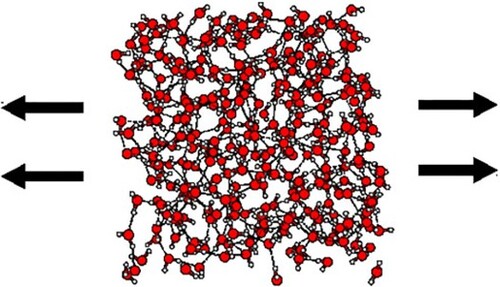
GRAPHICAL ABSTRACT

Keywords:

• Water
• pressure effects
• quantum simulations
• mechanical instability
• spinodal line

1. Introduction

In recent decades, the experimentally accessible domain within the phase diagrams of diverse substances has considerably expanded. This enlargement has provided a more profound comprehension of condensed phases subjected to extreme conditions of temperature and pressure, as documented by various studies [1,2]. Consequently, there has been an in-depth exploration of how different properties of condensed matter respond to hydrostatic pressure. This scrutiny extends to a growing interest in tensile stress, a factor that holds the potential to enhance our understanding of the metastability boundaries inherent in various phases. [3–6]. This contributes to the refinement of our knowledge about the behaviour of condensed matter under extreme conditions and provides insights into the attractive region of intermolecular forces.

Over the years, the high-pressure region of the phase diagram for water has garnered significant interest within the realms of condensed matter physics, chemistry, and planetary sciences, as evidenced by a body of research [7–11]. This attention is not only attributed to the intrinsic importance of water, but is also motivated by the multitude of ice polymorphs discovered under varying conditions of temperature (T) and pressure (P). To date, investigations into the phase diagram of water have been extended to temperatures up to $T\sim 1000$ K and pressures reaching several hundreds of GPa [12].

The examination of condensed matter behaviour under tensile pressure has predominantly focussed on liquids [3,13–17]. These investigations delve into the mechanical stability limits and the occurrence of cavitation in proximity to their spinodal lines. In recent years, the experimentally accessible domain of hydrostatic (or quasi-hydrostatic) tensile pressure has significantly enlarged. This expansion has not only widened the scope of study, but has also deepened our understanding of physical properties under conditions that pose challenges in laboratory settings [3,18–22].

Liquid water under tensile pressure has undergone extensive scrutiny in recent years, with both theoretical investigations, primarily through simulations [23–32], and experimental studies [3,33–38]. Numerous inquiries have focussed on identifying thermodynamic and mechanical anomalies within stretched water. Variables such as density, compressibility, and sound velocity have been subject to exploration in various works [34,38–43]. Noteworthy attention has been given to investigating the phenomenon of water cavitation under negative pressure, wherein the metastable liquid undergoes breakdown through the nucleation of vapor bubbles [33,44–48]. Within this context, several studies have delved into the liquid-gas spinodal line of water [23,26,28,42,49,50].

In this paper, we focus on the properties of water under negative pressure. Our main goal is to gain insight into the influence of nuclear quantum motion on such properties, particularly on the liquid-gas spinodal line. To achieve this, we have carried out extensive path-integral molecular dynamics (PIMD) simulations using a reliable interatomic potential (q-TIP4P/F), suitable for this type of simulations. We find that the spinodal pressure changes by 15 and 10 MPa at T = 250 and 300 K, respectively, as compared with the results of classical molecular dynamics simulations. Quantum effects are also analysed for the molar volume, structure of water molecules, as well as internal and kinetic energy of the liquid in the region of negative pressure. Similar techniques based on atomistic simulations have been employed earlier to study the mechanical stability of solids [51–53].

The paper is structured as follows: In Section 2, we detail the computational method utilised in our calculations. Section 3 is dedicated to the discussion of kinetic and internal energy as functions of pressure and temperature. Structural properties, including the O–H bond length and H–O–H angle, are examined in Section 4, while Section 5 delves into the molar volume. The liquid-gas spinodal instability is explored in Sections 6, and 7 summarises the main results.

2. Computational method

In this study, we employ the PIMD computational technique to investigate the properties of water across a range of temperatures and pressures, encompassing both compression (P>0) and tension (P<0) conditions. The foundation of this approach lies in an isomorphism established between the actual quantum system and an artificial classical counterpart, which emerges through the discretization of the quantum density matrix along cyclic paths [54,55]. This isomorphism is practically realised by substituting each quantum particle with a ring polymer composed of $N_{\mathrm{Tr}}$ (Trotter number) classical pseudo-particles. These pseudo-particles are interconnected by harmonic springs with force constants that vary with mass and temperature. The isomorphism is exact for $N_{\mathrm{Tr}}\to \mathrm{\infty }$, but in practical applications, the choice of $N_{\mathrm{Tr}}$ involves a trade-off between accuracy (increasing $N_{\mathrm{Tr}}$) and computational feasibility (reducing $N_{\mathrm{Tr}}$). Further details on this simulation method can be found in previous works [56–58].

The dynamics observed in PIMD simulations are inherently artificial, as they do not faithfully capture the genuine quantum dynamics of atomic nuclei. However, despite this artificiality, PIMD simulations serve as a practical and potent approach for effectively exploring the many-body configuration space. This capability enables the generation of precise data regarding the equilibrium properties of the actual quantum system. An alternative method for computing equilibrium properties relies on Monte Carlo sampling. Nonetheless, this approach demands greater computational resources, notably in terms of CPU time, compared to the PIMD method, which holds an advantage in this context due to its enhanced parallelisation potential. This feature is crucial for optimising the efficiency of operations on modern computer architectures.

For our water simulations, we employed the point charge, flexible q-TIP4P/F potential model to describe interatomic interactions. This model has been demonstrated to be particularly suitable for analysing nuclear quantum effects in the structural, dynamical, and thermodynamic properties of water [59]. Notably, it has been applied to investigate various states of water, including the liquid phase [59–63], ice [64–69], clusters [70], and the phase diagram [71]. Furthermore, the same model has been recently utilised to examine a liquid-liquid phase transition in water [72].

Other simulations investigating condensed phases of water have relied on empirical potentials that treat H${}_2$O molecules as rigid entities [73–75]. While this approach can offer computational efficiency and produce satisfactory results for various properties of the liquid state and various ice polymorphs, it overlooks the impact of molecular flexibility on the dynamics and structure of different phases [59]. For instance, employing flexible H${}_2$O molecules allows for the exploration of correlations between intramolecular O–H bond distances ($d_{\mathrm{O}-\mathrm{H}}$) and the geometry of intermolecular H bonds, a phenomenon extensively studied in ice [76–78]. Additionally, incorporating anharmonic stretches in the q-TIP4P/F potential enables the examination of variations in the $d_{\mathrm{O}-\mathrm{H}}$ distance as a function of both temperature and pressure. This approach further facilitates the discernment of differences between data derived from classical and quantum simulations.

Most of the water simulations discussed herein were conducted within the isothermal-isobaric NPT ensemble. This choice facilitated the determination of the equilibrium volume of the liquid under specified pressure and temperature conditions. The PIMD simulations in this statistical ensemble were executed using algorithms detailed in the literature [79–82]. Staging variables were employed to define the bead coordinates, and a constant temperature was maintained by coupling chains of four Nosé-Hoover thermostats to each staging variable. Additionally, a chain incorporating four barostats was connected to the volume to uphold the desired pressure, as described by Tuckerman and Hughes [80]. The pressure was calculated using a virial expression suitable for PIMD simulations [58]. Near the liquid-gas spinodal (negative) pressure, $P_s$, we also conducted PIMD simulations in the canonical (NV T) ensemble. This approach allowed for extended simulations of metastable liquid water in a region of the phase diagram where NPT simulations tend to become rapidly unstable.

For our simulations, we utilised cubic cells containing 300 water molecules with periodic boundary conditions. Configuration space sampling was conducted over a temperature range of 250 K to 375 K and pressures ranging from $-0.3$ to 1 GPa. The Trotter number was chosen to be proportional to the inverse temperature, specifically satisfying $N_{\mathrm{Tr}}T=6000$ K. Electrostatic interactions in the q-TIP4P/F potential were calculated by the Ewald method. The equations of motion were integrated using the reversible reference system propagator algorithm (RESPA), allowing for the use of different time steps for the integration of slow and fast dynamical variables [79]. Interatomic forces were computed with a time interval of $\mathrm{\Delta }t=0.2$ fs, which demonstrated acceptable convergence for the considered variables. In a typical simulation run at a given temperature T and pressure P, we performed ${10}^5$ PIMD steps for system equilibration and subsequently conducted $8\times {10}^6$ steps for computing average properties. For NV T simulations near the liquid-gas spinodal, runs included $2\times {10}^7$ steps to enhance statistics in the region of negative pressure. Other technical details about the simulations presented here were previously described in [65,67].

To evaluate the extent of quantum effects in the outcomes of PIMD simulations, we carried out classical molecular dynamics (MD) simulations of water employing the same interatomic potential q-TIP4P/F. In our context, this is akin to setting the Trotter number $N_{\mathrm{Tr}}$ equal to 1.

3. Energy

In this section, we delve into the internal energy of water, derived from our PIMD simulations, with particular emphasis on the kinetic energy component. As an additional check of the potential model, we computed the heat capacity, $c_p$, by numerically differentiating the enthalpy $H=E+\mathrm{PV}$, i.e. $c_p=\mathrm{d}H/\mathrm{d}T$. Figure 1 illustrates the temperature-dependent behaviour of $c_p$ at a constant pressure of 1 bar, featuring results obtained from both classical MD simulations (depicted by circles) and PIMD simulations (shown as squares). Within this figure, diamonds symbolise the experimental heat capacity of water at several temperatures, given by Angell et al. [83]. The classical MD results overestimate the actual heat capacity, exhibiting a decreasing trend with rising temperature throughout the displayed temperature range in Figure 1. This trend reduces the disparity with the quantum data. On the other hand, the outcomes of PIMD simulations align more closely with the experimental values, although they fall slightly below the latter. This difference exceeds the error bar associated with the simulation data.

Figure 1. Heat capacity of water as a function of temperature, as derived from classical MD (circles) and PIMD simulations (squares). Diamonds indicate experimental values given by Angell et al. [83], denoted as ‘exper.’. Dashed lines are guides to the eye.

We note that using alternative effective potentials for classical simulations can yield better agreement with known properties of water, as compared to the q-TIP4P/F potential in our classical simulations [84]. In this line, one could contrast results of classical and PIMD simulations utilising different potentials, but this can hinder a direct assessment of quantum effects. This is because such effects could be confounded by the inherent distinctions between the interatomic potentials themselves. Our goal is mainly centred on quantifying the magnitude of nuclear quantum effects, assuming a reliable interatomic potential, rather than discerning between the quality of various potentials.

Path integral simulations offer distinct estimators for the potential ($E_p$) and kinetic energy ($E_k$) of a system. In the domain of molecular and condensed-matter physics, the kinetic energy of an atomic nucleus depends not only on temperature but also on its mass and spatial delocalisation. Classical physics posits that each degree of freedom contributes to the kinetic energy per mole in an amount proportional to the temperature, specifically $RT/2$ (where R is the gas constant), aligning with the equipartition principle. However, the quantum kinetic energy is linked to the potential landscape surrounding the particle under consideration. Path integral simulations emerge as an apt technique for computing $E_k$ of quantum particles, providing insights into the dispersion of quantum paths. In particular, the radius-of-gyration of the cyclic paths becomes an important factor, as a larger radius-of-gyration corresponds to greater quantum delocalisation, resulting in a reduction of $E_k$ [56,65]. We have undertaken the calculation of $E_k$ in water using the virial estimator, acknowledged for its statistical precision [80,85], yielding error bars smaller than those associated with the potential energy, especially at elevated temperatures [61,86]. The kinetic energy of hydrogen in water at atmospheric pressure was previously studied in detail through PIMD simulations, especially in connection with deep inelastic neutron-scattering experiments [61].

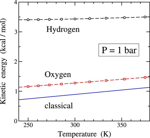
In Figure 2, we present the kinetic energy per mole of oxygen (depicted as squares) and hydrogen (depicted as circles) as a function of temperature, calculated from our PIMD simulations performed at P = 1 bar. $E_k^{\mathrm{H}}$ for hydrogen atoms is clearly larger than for oxygen atoms, $E_k^{\mathrm{O}}$, as expected for the smaller mass of the former. Within the temperature range illustrated in Figure 2, the ratio $E_k^{\mathrm{H}}/E_k^{\mathrm{O}}$ decreases from 3.0 to 2.4. The cumulative kinetic energy of water, $E_k=2E_k^{\mathrm{H}}+E_k^{\mathrm{O}}$, exhibits an ascent from 7.93 kcal/mol at 250 K to 8.46 at 375 K, with $E_k=8.14$ kcal/mol at 300 K. The solid line in Figure 2 represents the classical value of $E_k^{\mathrm{O}}$ or $E_k^{\mathrm{H}}$, i.e. $E_k^{\mathrm{cl}}=3RT/2$. In the temperature range depicted in this figure, the quantum kinetic energy of oxygen gradually converges toward the classical value as T increases. However, the former still remains noticeably greater than the latter at temperatures around 400 K.

Figure 2. Kinetic energy as a function of temperature for P = 1 bar, derived from PIMD simulations for hydrogen (circles) and oxygen (squares) in water. Error bars are smaller than the symbol size. The solid line indicates the classical value: $E_k^{\mathrm{cl}}=3\mathrm{RT}/2$. Dashed lines are guides to the eye.

We now explore the pressure-dependent behaviour of the internal and kinetic energy of water. In Figure 3, we display the internal energy, $E=E_p+E_k$, as a function of pressure, derived from our PIMD simulations utilising the q-TIP4P/F interatomic potential for $P\le 0$. The energy scale in this plot aligns with the original parameterisation of the potential model [59]. With an increasing tensile pressure, the internal energy steadily rises until P reaches values around $-0.22$ GPa, where a prominent cusp appears. This cusp signifies the proximity to the mechanical instability of the liquid. The elevation of energy under increasing tensile pressure primarily results from the growth of the system's potential energy, which distinctly dominates over the decrease in kinetic energy, as illustrated in Figure 4. The vertical dashed-dotted line in Figure 3 represents the critical pressure $P_s=-0.236$ GPa, denoting the limit of mechanical stability at T = 300 K, as explained in Section 6.

Figure 3. Pressure dependence of the energy for T = 300 K (circles). Symbols represent results of PIMD simulations. Error bars are on the order of the symbol size. The dashed line is a guide to the eye. A vertical dashed-dotted line indicates the pressure of mechanical instability at 300 K.

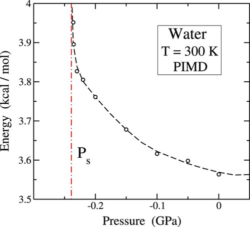
Figure 4. Kinetic energy as a function of pressure for T = 300 K, calculated from PIMD simulations. (a) Oxygen (open circles); (b) hydrogen (open squares). Error bars in (a) are on the order of the symbol size. The dashed lines are guides to the eye.

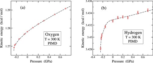
In Figure 4, we show the kinetic energy evolution of (a) oxygen and (b) hydrogen atoms at 300 K as a function of P, encompassing compressive and tensile stress conditions. For both atomic species, there is a discernible augmentation in $E_k$ as compressive stress intensifies, indicative of $\mathrm{d}{E}_k/\mathrm{d}P>0$. This positive derivative persists under tensile stress (P<0); however, its magnitude undergoes a rapid surge around P = −0.2 GPa. This pronounced increase is particularly conspicuous for hydrogen, especially in close proximity to the mechanical instability of water.

For a given temperature, an elevation in kinetic energy correlates with a reduction in the dispersion of quantum paths, as indicated by the decrease in the radius-of-gyration associated with the considered atomic nucleus. Consequently, both O and H paths contract under increasing compressive pressure and expand under tensile stress. The upward trend exhibited by the kinetic energy for P>0 aligns with the typical pattern of heightened vibrational frequencies observed with increasing pressure in condensed matter. However, it is noteworthy that the change in $E_k^{\mathrm{O}}$ and $E_k^{\mathrm{H}}$ throughout the entire pressure range depicted in Figure 4 is considerably smaller than the growth observed in Figure 2 when temperature increases from 250 to 375 K, specifically 0.31 and 0.09 kcal/mol for oxygen and hydrogen, respectively.

4. Molecular geometry

In this section we present results for the molecular geometry of water, which can shed light on the structural changes suffered by the liquid when temperature or pressure are modified. We concentrate on the intramolecular O–H bond length and the H–O–H angle.

4.1. O–H bond

Figure 5 illustrates the temperature and pressure dependencies of the bond distance $d_{\mathrm{O}-\mathrm{H}}$ in water, as determined through classical and quantum simulations using the q-TIP4P/F potential model. In Figure 5(a) the mean distance $d_{\mathrm{O}-\mathrm{H}}$ is presented as a function of temperature at P = 1 bar. Simulation results are denoted by open symbols, with circles representing classical MD and squares corresponding to PIMD. Classical and quantum simulations exhibit a similar temperature dependence, as depicted by the trends observed in results for both cases.

Figure 5. (a) Intramolecular O–H distance, $d_{\mathrm{O}-\mathrm{H}}$, vs temperature for P = 1 bar, as derived from simulations with the q-TIP4P/F potential. (b) $d_{\mathrm{O}-\mathrm{H}}$ as a function of pressure for T = 300 K. In both panels, circles and squares represent results of classical MD and PIMD simulations, respectively. Error bars are in the order of the symbol size. Lines are guides to the eye.

In Figure 5(a) it is clear that the mean distance $d_{\mathrm{O}-\mathrm{H}}$ resulting from quantum simulations surpasses that obtained in classical simulations. Specifically, for water the disparity between the two datasets is 0.014 Å (1.4% of the bond length), and this difference marginally diminishes by less than ${10}^{-3}$ Å within the considered temperature range. At T = 300 K, the rate of change of $d_{\mathrm{O}-\mathrm{H}}$ with respect to temperature is $\mathrm{\partial }{d}_{\mathrm{O}-\mathrm{H}}/\mathrm{\partial }T=-2.7\times {10}^{-5}$ Å/K for classical results and $-3.1\times {10}^{-5}$ Å/K for the quantum data. Notably, the bond expansion induced by nuclear quantum motion mirrors findings observed in analogous PIMD simulations for ice Ih [67].

We highlight a noteworthy observation in our findings: the decrease in $d_{\mathrm{O}-\mathrm{H}}$ as temperature rises. At first glance, this may appear counterintuitive, especially considering the conventional understanding of thermal expansion in atomic bonds. The counterintuitive nature of this trend becomes more apparent when considering the expected expansion associated with an increase in volume. However, our results unveil an intriguing and seemingly anomalous behaviour that aligns with observations in various water phases, where the covalent O–H bond contracts with rising temperature ($\mathrm{\partial }{d}_{\mathrm{O}-\mathrm{H}}/\mathrm{d}T<0$). This behaviour arises from a delicate interplay between the general tendency of bond distances to increase with temperature and the opposing effect caused by the fortification of the intramolecular O–H bond. This fortification is linked to a weakening of intermolecular H bonds, resulting from a larger mean O–O distance and the consequential expansion of volume. In essence, our findings agree with the local intra-intermolecular geometric correlation identified in both liquid and solid water. This correlation relates the intramolecular O–H bond length to the corresponding H-bond geometry [76,77]. Similar effects on $d_{\mathrm{O}-\mathrm{H}}$ have been previously documented in PIMD simulations of ice VII using the q-TIP4P/F potential model [69].

Considering the aforementioned arguments, we anticipate an increase in the bond distance $d_{\mathrm{O}-\mathrm{H}}$ under increasing compressive pressure. In this scenario, the reduction in volume leads to a contraction of intermolecular H bonds, consequently causing the expansion (weakening) of intramolecular bonds. This relationship is illustrated in Figure 5(b), where $d_{\mathrm{O}-\mathrm{H}}$ is plotted against hydrostatic pressure P. The figure reveals a consistent trend across classical and quantum datasets, showing that $d_{\mathrm{O}-\mathrm{H}}$ expands with increasing compression and contracts with growing tensile pressure. The difference between the two datasets remains constant within the pressure range depicted in Figure 5(b), totalling 0.014 Å. For P>0, the change in $d_{\mathrm{O}-\mathrm{H}}$ is characterised by a slope $\mathrm{\partial }{d}_{\mathrm{O}-\mathrm{H}}/\mathrm{\partial }P=1.0\times {10}^{-3}$ Å/GPa, observed consistently in both classical and quantum results. Conversely, for P<0 a reduction in the bond distance is observed, accelerating as the system approaches mechanical instability at $P\sim -0.24$ GPa. At the scale of Figure 5(b), this reduction does not exhibit as sharp a transition as observed in the kinetic energy presented in Figure 4.

We observe that variations in the interatomic distance $d_{\mathrm{O}-\mathrm{H}}$, depicted in Figure 5(a,b), appear relatively minor. However, they are comparable to discrepancies observed among intramolecular distances in different ice phases [69]. Moreover, these changes may hold significance in elucidating variations in vibrational frequencies within water under varying external conditions.

4.2. H–O–H angle

In Figure 6(a), we present a comprehensive analysis of the temperature-dependent behaviour of the mean H–O–H angle, denoted as ${\theta }_{\mathrm{H}-\mathrm{O}-\mathrm{H}}$, in water molecules, carried out using classical MD (represented by circles) and PIMD simulations (indicated by squares). Our results at 300 K are in agreement with the findings from Refs. [59,64], where the q-TIP4P/F interatomic potential was employed.

Figure 6. Mean angle ${\theta }_{\mathrm{H}-\mathrm{O}-\mathrm{H}}$ obtained from simulations with the q-TIP4P/F potential. (a) Temperature dependence for P = 1 bar; (b) Pressure dependence for T = 300 K. Circles and squares indicate results of classical MD and PIMD simulations, respectively. Lines are guides to the eye.

Upon examination of both classical and quantum datasets in Figure 6(a), a consistent pattern emerges: an observable reduction in the angle ${\theta }_{\mathrm{H}-\mathrm{O}-\mathrm{H}}$ as the temperature is elevated. This fact holds significance for understanding the thermal dynamics of water molecules. A decrease in ${\theta }_{\mathrm{H}-\mathrm{O}-\mathrm{H}}$ for rising T was also found by Gu et al. from classical MD simulations using the MCYL potential [87]. Furthermore, our investigation reveals that nuclear quantum motion induces a subtle but discernible diminution in the intramolecular angle, approximately 0.1 deg., with this effect becoming less pronounced at higher temperatures. This interplay between temperature and quantum effects sheds light on the dynamical aspects of the water molecule behaviour in the liquid phase. At T = 300 K, we find $\mathrm{\partial }{\theta }_{\mathrm{H}-\mathrm{O}-\mathrm{H}}/\mathrm{\partial }T=-8.6\times {10}^{-4}$ deg./K and $-6.1\times {10}^{-4}$ deg./K from our classical and quantum results, respectively. The change with the temperature is larger for the classical model, and both sets of results approach to each other as T rises.

Expanding our analysis to include the effect of pressure, Figure 6(b) showcases the mean angle ${\theta }_{\mathrm{H}-\mathrm{O}-\mathrm{H}}$ under compressive and tensile pressure conditions. Both classical (circles) and quantum (squares) simulations at T = 300 K present a decrease in the mean angle for rising P, i.e. $\mathrm{\partial }{\theta }_{\mathrm{H}-\mathrm{O}-\mathrm{H}}/\mathrm{\partial }P<0$, in the whole range of pressure under consideration. At atmospheric pressure, we obtain from our simulations a pressure derivative $\mathrm{\partial }{\theta }_{\mathrm{H}-\mathrm{O}-\mathrm{H}}/\mathrm{\partial }P=-0.26(1)$ deg./GPa for both the classical and quantum data, which coincide within the precision of our numerical procedure. This slope clearly becomes less negative as compressive pressure is raised. On the contrary, when subjected to increasing tensile stress within the mechanical stability region of the liquid phase, the mean angle ${\theta }_{\mathrm{H}-\mathrm{O}-\mathrm{H}}$ exhibits growth. This response to compressive and tensile pressures provides insight into the structural adaptability of water molecules under different conditions.

A noteworthy observation is the amplification of the negative slope in the vicinity of the stability limit ($P\sim -0.24$ GPa). This indicates a heightened sensitivity of the H–O–H angle to pressure variations, especially in the proximity of the spinodal pressure $P_s$ corresponding to each approach (classical or quantum).

Water molecules within the crystal structures of diverse ice phases exhibit a notable range in bond angles, spanning from 96.4 to 112.8 deg. For isolated water molecules, detailed quantum-mechanical calculations [88] have unveiled a discernible negative correlation between the distance $d_{\mathrm{O}-\mathrm{H}}$ and the angle ${\theta }_{\mathrm{H}-\mathrm{O}-\mathrm{H}}$. This correlation aligns with the observed pressure dependence in liquid water, illustrated in Figures 5(b) and 6(b). In contrast, from the temperature dependence analysis of both structural variables we find a positive correlation, as portrayed in Figures 5(a) and 6(a) (mean bond length and angle decrease for rising T). This can be related to an expanding dispersion in the actual bond and angle distributions as temperature increases [63].

To conclude this section, it is noteworthy that changes in the angle ${\theta }_{\mathrm{H}-\mathrm{O}-\mathrm{H}}$, as depicted in Figure 6(a,b), are relatively small. Specifically, they remain under 0.2 deg. across all scenarios. Nevertheless, despite their subtlety, these variations can significantly influence the bending mode of water, particularly depending on the prevailing temperature and pressure conditions [89,90].

5. Pressure-volume equation of state

The q-TIP4P/F potential model has been demonstrated to provide accurate results for the temperature dependence of the molar volume of water, using path-integral simulations. Specifically, it predicts a temperature of maximum density of 280 K, in reasonable agreement with experimental data [59,63,64]. The molar volume derived from PIMD simulations is larger than that obtained in classical simulations, leading to a concomitant reduction in water density, as indicated earlier [64]. We have verified that our results for the temperature dependence of the molar volume, as well as the isothermal compressibility ${\kappa }_T$, at room conditions (T = 300 K, P = 1 bar) agree with those obtained earlier using PIMD with the q-TIP4P/F interatomic potential [63,64].

Under tensile stress, the molar volume of water steadily increases in the pressure range of mechanical stability. In Figure 7, we display a graphical representation illustrating the relationship between molar volume and tensile pressure, as determined through classical simulations conducted at three distinct temperatures: T = 300 K (represented by circles), 340 K (depicted by squares), and 375 K (indicated by diamonds). The molar volume exhibits an accelerated increase with rising tensile pressure, culminating in the proximity of the mechanical instability specific to each temperature.

Figure 7. Molar volume of water as a function of pressure at three temperatures: T = 300 K (circles), 340 K (squares), and 375 K (diamonds). Symbols indicate results of classical MD simulations. Error bars are on the order of the symbol size. Dashed lines are guides to the eye. The vertical dashed-dotted lines indicate the estimated spinodal pressure for each temperature.

For better clarity, vertical dashed-dotted lines have been incorporated in the graph, denoting the spinodal pressure $P_s$ corresponding to each temperature. At $P_s$, the rate of change of volume with respect to pressure, $(\mathrm{\partial }V/\mathrm{\partial P}{)}_T$, approaches $-\mathrm{\infty }$, signifying a singular point. The simulations are unable to approach this limit, and the vertical dashed-dotted lines serve as markers for this theoretical boundary.

Furthermore, we note that, for each temperature in Figure 7, the three data points in closest proximity to the spinodal pressure were obtained from NV T simulations. The considerable volume fluctuations observed in NPT simulations near the liquid-gas spinodal pressure impede an effective sampling of that region of the configuration space. This limitation becomes more pronounced at elevated temperatures, where the concurrent increase in volume fluctuations increases the difficulty of accurately exploring the system. To address this question, we have carried out simulations in the canonical ensemble in the segments of the configuration space where liquid water maintains a metastable state throughout sufficiently extended simulation runs. This ensures that the system remains within the metastable phase of liquid water for a duration conducive to the precise sampling of structural and thermodynamic variables. By leveraging NV T simulations in these specific regions, we avoid the impact of volume fluctuations, allowing for a more reliable and comprehensive exploration of the targeted configuration space, close to the spinodal pressure at the considered temperatures.

In Figure 8, we present the pressure-dependent behaviour of the molar volume of water, derived from simulations utilising the q-TIP4P/F potential at a temperature of 250 K. The symbols in the graph represent simulation outcomes, with circles denoting classical MD and squares indicating PIMD simulations. Within error bars, a coincidence between classical and quantum results is observed for P>−0.1 GPa, aligning with previous findings [63] at the same temperature. However, as tensile pressure increases, a noteworthy divergence emerges, with quantum simulations yielding volumes surpassing their classical counterparts. This deviation intensifies with increasing tensile pressure, ultimately culminating in a manifestation of mechanical instability at lower tension in the quantum simulations.

Figure 8. Pressure dependence of the molar volume of water at $T=250$ K. Symbols represent results of classical MD (circles) and PIMD simulations (squares). Error bars are in the order of the symbol size. Lines are guides to the eye. Vertical dashed-dotted lines indicate the spinodal pressure for each approach.

From these results we estimate for the liquid-gas spinodal pressure $P_s$ values of $-301$ and $-286$ MPa for the classical and quantum approaches, respectively. These $P_s$ values are shown in Figure 8 as vertical dashed-dotted lines. We find that nuclear quantum dynamics causes a shift in the spinodal pressure of 15 MPa at T = 250 K. This shift is smaller for higher temperatures, as shown below.

According to the results of our simulations, this trend persists across a region of temperatures ranging from 250 to 375 K. It is noteworthy that while the quantum effect on the spinodal pressure is discernible across this temperature range, its influence diminishes with rising temperature. At T = 375 K, the quantum impact on the spinodal pressure becomes notably subtle, approaching the limits of observability in our results. This temperature-dependent behaviour elucidates the interplay between quantum effects, temperature, and mechanical stability, providing valuable insights into the thermodynamic properties of water under varying conditions.

6. Spinodal instability

The liquid expansion caused by tensile stress gives rise to a fast increase in the compressibility, which diverges for a temperature-dependent pressure $P_s$, where liquid water becomes mechanically unstable. This is typical of a spinodal point in the $(P,T)$ phase diagram [51,91–93]. Given a temperature T, there is a region of tensile pressure where liquid water is metastable, specifically, for $P_s<P<0$. The spinodal line, delineating the unstable phase ($P<P_s$) from the metastable phase, is the locus of points $P_s(T)$ where ${\kappa }_T$ diverges, or equivalently, where its inverse, the isothermal bulk modulus, vanishes. This type of spinodal line has been previously investigated for water [26,28,33,42,49,50,94,95], as well as for various types of solids [51,52,91]. In recent years, research has explored this question in two-dimensional materials, where this type of instability may also be found under compressive stress [92,96].

Close to a spinodal point, the Helmholtz free energy F at temperature T can be written as a Taylor power expansion in terms of the volume difference $V_s-V$ [14,94,96]: (1) $\begin{array}{rl}F(V,T)& =F(V_s(T),T)+{\alpha }_1(T)[V_s(T)-V]\\ & +{\alpha }_3(T)[V_s(T)-V{]}^3+\cdots .\end{array}$(1) Here $V_s(T)$ and $F(V_s(T),T)$ are the volume and free energy at the spinodal point, where one has ${\mathrm{\partial }}^{2}F/\mathrm{\partial }{V}^2=0$, and a quadratic term $[V_s(T)-V{]}^2$ does not appear in Equation (1(1) $\begin{array}{rl}F(V,T)& =F(V_s(T),T)+{\alpha }_1(T)[V_s(T)-V]\\ & +{\alpha }_3(T)[V_s(T)-V{]}^3+\cdots .\end{array}$(1) ): ${\alpha }_2=0$. The coefficients ${\alpha }_i$ along with the spinodal volume $V_s$ depend in general on the temperature, although we will not explicitly write this dependence in the sequel. The pressure is given by (2) $P=-\frac{\mathrm{\partial }F}{\mathrm{\partial }V}=P_s+3{\alpha }_3(V_s-V{)}^2+\cdots ,$(2) and $P_s={\alpha }_1$ corresponds to the spinodal pressure and to the volume $V_s$.

The isothermal compressibility ${\kappa }_T$ is obtained as (3) ${\kappa }_T=\frac{1}{V}{\left(\frac{{\mathrm{\partial }}^{2}F}{\mathrm{\partial }{V}^2}\right)}^{-1}=-\frac{1}{V}{\left(\frac{\mathrm{\partial }P}{\mathrm{\partial }V}\right)}_T^{-1},$(3) and one has for P close to $P_s$: (4) ${\kappa }_T\sim (P-P_s{)}^{-1/2}.$(4) The compressibility diverges to infinity for $P\to P_s$, as the inverse square root of $P-P_s$.

In Figure 9 we display the liquid-gas spinodal pressure $P_s$ of water as a function of the temperature, estimated from our classical (circles) and PIMD simulations (squares). We observe a decrease in $P_s$ as the temperature is lowered into the region of supercooled water. Our classical results can be fitted to a straight line $P_s=b_1+b_{2}T$, with $b_1=-591$ MPa and $b_2=1.15$ MPa/K (shown as the dashed-dotted line in Figure 9). Consequently, we do not detect any indication of reentrant behaviour (an increase in $P_s$ at low temperatures), in agreement to findings in Refs. [26,28] from classical MD simulations. The anticipated reentrant spinodal, extrapolated from various thermodynamic properties of water [95], according to the stability-limit conjecture, suggests that the spinodal pressure should decrease upon cooling, become negative, and then increase after reaching a minimum [33,95]. However, our simulation data are in line with the model proposed by Poole et al. [23], where the spinodal remains positively sloped and extends to larger negative pressures when lowering the temperature.

Figure 9. Temperature dependence of the spinodal pressure, $P_s$, derived from classical MD (solid circles) and PIMD simulations (solid squares). The dashed-dotted line is a linear fit to the classical data. The dashed line through the quantum outcomes is a guide to the eye.

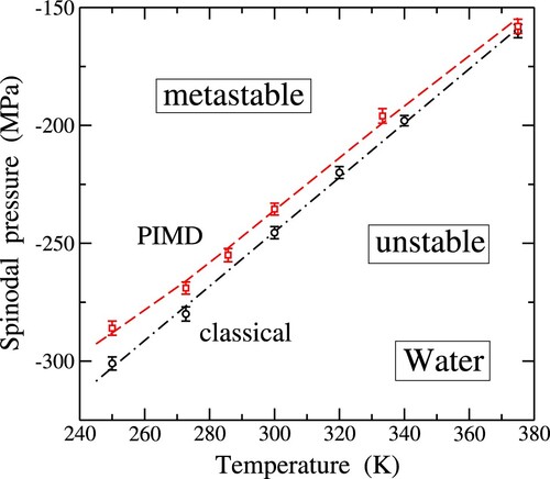
From the outcomes of our PIMD simulations, we observe that nuclear quantum dynamics induces a positive shift in the liquid-gas spinodal pressure within the considered temperature range. Specifically, we find shifts of 10 and 15 MPa at temperatures of 300 and 250 K, respectively (resulting in $P_s$ becoming less negative). Our quantum data appear to deviate slightly from linearity, especially at the lowest temperatures depicted in Figure 9. The quantum effect on $P_s$ is found to increase as T is lowered, mirroring trends seen in other physical variables calculated from path integral simulations.

As indicated in the plot, in each case, classical or quantum, the liquid exhibits metastability at negative pressures in the region above the corresponding dashed-dotted or dashed line. Below it, the liquid becomes mechanically unstable, leading to a transformation into the gas phase, where the volume diverges to infinity under tensile pressure. When approaching the line (classical or quantum) from the metastable region, the transition may occur well before reaching the spinodal. This phenomenon was clearly observed in our isothermal-isobaric simulations when increasing the tensile stress near the spinodal.

Our classical results for the liquid-gas spinodal pressure are not far from those obtained by Netz et al. [28] from MD simulations using the SPC/E potential model. Specifically, these authors reported a value of approximately $-270$ MPa at T = 250 K, compared to our value of $-301$ MPa at the same temperature. Gallo et al. [26] conducted MD simulations of stretched water employing a polarisable potential model, and from their spinodal pressure results, we interpolate a value of about $-330$ MPa at T = 250 K. The $P_s$ value derived from our classical MD simulations at this temperature falls intermediate between those obtained using these other potential models.

More recently, Biddle et al. [41] employed the TIP4P/2005 interatomic potential to study the thermodynamics of water in a wide range of temperature and pressure, using classical MD simulations. From the results presented in their Figure 1, we estimate at T = 250 and 300 K values of $P_s\approx -310$ and $-240$ MPa, to be compared with the outcomes of our classical simulations: $-301$ and $-246$ MPa, respectively. A smaller value for the spinodal pressure at 300 K, $P_s\approx -175$ MPa was found in [23] from an extrapolation of P−V isotherms at negative P, derived by using MD simulations with the ST2 pair potential.

7. Summary

In this paper, we have presented the outcomes of PIMD simulations for liquid water, under various hydrostatic pressures encompassing both compressive and tensile regimes. These quantum simulations, carried out at a specific temperature, afford a comprehensive analysis of water within pressure ranges where it exhibits stability or metastability. Through this methodology, we have quantitatively examined several properties of water, with a particular focus on delineating its mechanical stability limit.

The significance of quantum effects has been evaluated by contrasting the findings derived from PIMD simulations with those emanating from classical MD simulations. Specifically, we have employed the q-TIP4P/F interatomic potential, which has proved to be well-suited for this kind of investigations. This potential model adeptly captures numerous structural and thermodynamic features across distinct water phases, underscoring its applicability and reliability in elucidating the intricate behaviour of water molecules.

While the molar volume of water experiences a reduction under increased compression at a constant temperature, the interatomic distances exhibit a distinct pattern, characteristic of various condensed phases of water. Notably, the interatomic distance between oxygen atoms in adjacent water molecules decreases with rising compressive pressure, while the intramolecular distance $d_{\mathrm{O}-\mathrm{H}}$ concurrently increases, indicative of a simultaneous attenuation in the strength of the covalent bond.

Quantum nuclear motion induces changes in structural variables, prompting a detailed analysis of quantum effects on internal and kinetic energy, intramolecular distance $d_{\mathrm{O}-\mathrm{H}}$, bond angle ${\theta }_{\mathrm{H}-\mathrm{O}-\mathrm{H}}$, and molar volume as a function of pressure and temperature. Notably, our focus extends to P<0, particularly in proximity to the spinodal pressure corresponding to each considered temperature. The influence of quantum nuclear motion manifests in a discernible shift of the liquid-gas spinodal pressure, amounting to 15 and 10 MPa at temperatures of 250 and 300 K, respectively. Within this temperature range, our quantum simulations reveal $P_s$ values spanning from $-286$ to $-236$ MPa.

These findings underscore the interplay among temperature, pressure, and nuclear quantum motion in shaping the structural dynamics of water molecules. This insight not only provides a pathway for further exploration but also facilitates a deeper comprehension of the nuanced behaviours governing water at the molecular level. Such understanding holds potential implications across diverse fields, spanning from materials science to environmental studies.

The computational methodology outlined in this paper has demonstrated its reliability as a robust tool for elucidating the impact of pressure on metastable states within liquids. In particular, it facilitates the calculation of the spinodal line under tensile stress as a temperature-dependent function. Future investigations in this domain are essential to expand upon the results presented herein, especially in the context of other liquids. The stability limits of these liquids will hinge on the behaviour of their compressibility under tensile stress, warranting further exploration and analysis.

Disclosure statement

No potential conflict of interest was reported by the author(s).

Additional information

Funding

This work was supported by Ministerio de Ciencia e Innovación (Spain) through Grant PID2022-139776NB-C66.

References

- A. Mujica, A. Rubio, A. Munoz and R. Needs, Rev. Mod. Phys. 75, 863–912 (2003). doi:10.1103/RevModPhys.75.863.
- H.K. Mao, X.J. Chen, Y. Ding, B. Li and L. Wang, Rev. Mod. Phys. 90, 015007 (2018). doi:10.1103/RevModPhys.90.015007.
- K. Davitt, E. Rolley, F. Caupin, A. Arvengas and S. Balibar, J. Chem. Phys. 133, 174507 (2010). doi:10.1063/1.3495971.
- M. Iyer, V. Gavini and T.M. Pollock, Phys. Rev. B 89, 014108 (2014). doi:10.1103/PhysRevB.89.014108.
- J. Nie, S. Porowski and P. Keblinski, J. Appl. Phys. 126, 035110 (2019). doi:10.1063/1.5097626.
- A.R. Imre, A. Drozd-Rzoska, T. Kraska, S.J. Rzoska and K.W. Wojciechowski, J. Phys.: Condens. Matter 20, 244104 (2008).
- D. Eisenberg and W. Kauzmann, The Structure and Properties of Water (Oxford University Press, New York, 1969).
- V.F. Petrenko and R.W. Whitworth, Physics of Ice (Oxford University Press, New York, 1999).
- E. Sanz, C. Vega, J.L.F. Abascal and L.G. MacDowell, Phys. Rev. Lett. 92, 255701 (2004). doi:10.1103/PhysRevLett.92.255701.
- C.G. Salzmanna, J. Chem. Phys. 150, 060901 (2019). doi:10.1063/1.5085163.
- L. Zhang, H. Wang, R. Car and E. Weinan, Phys. Rev. Lett. 126, 236001 (2021). doi:10.1103/PhysRevLett.126.236001.
- A.N. Dunaeva, D.V. Antsyshkin and O.L. Kuskov, Solar Syst. Res. 44, 202–222 (2010). doi:10.1134/S0038094610030044.
- M.A. Solis and J. Navarro, Phys. Rev. B 45, 13080–13083 (1992). doi:10.1103/PhysRevB.45.13080.
- J. Boronat, J. Casulleras and J. Navarro, Phys. Rev. B 50, 3427 (1994). doi:10.1103/PhysRevB.50.3427.
- P. Jedlovszky and R. Vallauri, Phys. Rev. E 67, 011201 (2003). doi:10.1103/PhysRevE.67.011201.
- A.R. Imre, Phys. Status Solidi B 244, 893–899 (2007). doi:10.1002/pssb.v244:3.
- A.R. Imre, A. Drozd-Rzoska, A. Horvath, T. Kraska and S.J. Rzoska, J. Non-Cryst. Solids 354, 4157–4162 (2008). doi:10.1016/j.jnoncrysol.2008.06.033.
- S.J. Henderson and R.J. Speedy, J. Phys. Chem. 91, 3069–3072 (1987). doi:10.1021/j100295a085.
- D.E. Grade, J. Mech. Phys. Solids 36, 353 (1988). doi:10.1016/0022-5096(88)90015-4.
- E. Moshe, S. Eliezer, Z. Henis, M. Werdiger, E. Dekel, Y. Horovitz, S. Maman, I.B. Goldberg and D. Eliezer, Appl. Phys. Lett 76, 1555–1557 (2000). doi:10.1063/1.126094.
- D.J. Dunstan, N.W.A. Van Uden and G.J. Ackland, High Press. Res. 22, 773–778 (2002). doi:10.1080/08957950212441.
- W.M.H. Verbeeten, M. Sanchez-Soto and M.L. Maspoch, J. Appl. Polymer Sci. 139, e52295 (2022). doi:10.1002/app.v139.23.
- P.H. Poole, F. Sciortino, U. Essmann and H.E. Stanley, Nature 360, 324–328 (1992). doi:10.1038/360324a0.
- J.L.F. Abascal and C. Vega, J. Chem. Phys. 134, 186101 (2011). doi:10.1063/1.3585676.
- V. Bianco, P.M. de Hijes, C.P. Lamas, E. Sanz and C. Vega, Phys. Rev. Lett. 126, 015704 (2021). doi:10.1103/PhysRevLett.126.015704.
- P. Gallo, M. Minozzi and M. Rovere, Phys. Rev. E 75, 011201 (2007). doi:10.1103/PhysRevE.75.011201.
- A.R. Imre, A. Baranyai, U.K. Deiters, P.T. Kiss, T. Kraska and S.E. Quiones Cisneros, Int. J. Thermophys. 34, 2053–2064 (2013). doi:10.1007/s10765-013-1518-8.
- P.A. Netz, F.W. Starr, H.E. Stanley and M.C. Barbosa, J. Chem. Phys. 115, 344–348 (2001). doi:10.1063/1.1376424.
- G. Pallares, M.A. Gonzalez, J.L.F. Abascal, C. Valeriani and F. Caupin, Phys. Chem. Chem. Phys. 18, 5896–5900 (2016). doi:10.1039/C5CP07580G.
- M. Sega, B. Fabian, A.R. Imre and P. Jedlovszky, J. Phys. Chem. C 121, 12214–12219 (2017). doi:10.1021/acs.jpcc.7b02573.
- A. Singraber, T. Morawietz, J. Behler and C. Dellago, J. Phys.: Condens. Matter 30, 254005 (2018).
- H.E. Stanley, M.C. Barbosa, S. Mossa, P.A. Netz, F. Sciortino, F.W. Starr and M. Yamada, Physica. A. 315, 281–289 (2002). doi:10.1016/S0378-4371(02)01536-4.
- M.E.M. Azouzi, C. Ramboz, J.F. Lenain and F. Caupin, Nature Phys. 9, 38–41 (2013). doi:10.1038/nphys2475.
- G. Pallares, M.E.M. Azouzi, M.A. Gonzalez, J.L. Aragones, J.L.F. Abascal, C. Valeriani and F. Caupin, PNAS USA 111, 7936–7941 (2014). doi:10.1073/pnas.1323366111.
- A.D. Alvarenga, M. Grimsditch and R.J. Bodnar, J. Chem. Phys. 98, 8392–8396 (1993). doi:10.1063/1.464497.
- C. Qiu, Y. Krueger, M. Wilke, D. Marti, J. Ricka and M. Frenz, Phys. Chem. Chem. Phys. 18, 28227–28241 (2016). doi:10.1039/C6CP04250C.
- C.A. Stan, P.R. Willmott, H.A. Stone, J.E. Koglin, M. Liang, A.L. Aquila, J.S. Robinson, K.L. Gumerlock, G. Blaj, R.G. Sierra, S. Boutet, S.A.H. Guillet, R.H. Curtis, S.L. Vetter, H. Loos, J.L. Turner and F.J. Decker, J. Phys. Chem. Lett. 7, 2055–2062 (2016). doi:10.1021/acs.jpclett.6b00687.
- V. Holten, C. Qiu, E. Guillerm, M. Wilke, J. Ricka, M. Frenz and F. Caupin, J. Phys. Chem. Lett. 8, 5519–5522 (2017). doi:10.1021/acs.jpclett.7b02563.
- Y.E. Altabet, R.S. Singh, F.H. Stillinger and P.G. Debenedetti, Langmuir 33, 11771–11778 (2017). doi:10.1021/acs.langmuir.7b02339.
- F. Caupin, A. Arvengas, K. Davitt, M.E.M. Azouzi, K.I. Shmulovich, C. Ramboz, D.A. Sessoms and A.D. Stroock, J. Phys.: Condens. Matter 24, 284110 (2012).
- J.W. Biddle, R.S. Singh, E.M. Sparano, F. Ricci, M.A. Gonzalez, C. Valeriani, J.L.F. Abascal, P.G. Debenedetti, M.A. Anisimov and F. Caupin, J. Chem. Phys. 146, 034502 (2017). doi:10.1063/1.4973546.
- F. Caupin and M.A. Anisimov, J. Chem. Phys. 151, 034503 (2019). doi:10.1063/1.5100228.
- A. Zaragoza, C.S.P. Tripathi, M.A. Gonzalez, J.L.F. Abascal, F. Caupin and C. Valeriani, J. Chem. Phys. 152, 194501 (2020). doi:10.1063/5.0002745.
- M.A. Gonzalez, G. Menzl, J.L. Aragones, P. Geiger, F. Caupin, J.L.F. Abascal, C. Dellago and C. Valeriani, J. Chem. Phys. 141, 18C511 (2014). doi:10.1063/1.4896216.
- G. Menzl, M.A. Gonzalez, P. Geiger, F. Caupin, J.L.F. Abascal, C. Valeriani and C. Dellago, PNAS USA 113, 13582–13587 (2016). doi:10.1073/pnas.1608421113.
- F. Magaletti, M. Gallo and C.M. Casciola, Sci. Rep. 11, 20801 (2021). doi:10.1038/s41598-021-99863-z.
- I. Sanchez-Burgos, M.C. Muniz, J.R. Espinosa and A.Z. Panagiotopoulos, J. Chem. Phys. 158, 184504 (2023). doi:10.1063/5.0144500.
- C.P. Lamas, C. Vega, E.G. Noya and E. Sanz, J. Chem. Phys. 158, 124504 (2023). doi:10.1063/5.0139470.
- M. Duska, J. Chem. Phys. 152, 174501 (2020). doi:10.1063/5.0006431.
- A.R. Imre, G. Mayer, G. Hazi, R. Rozas and T. Kraska, J. Chem. Phys. 128, 114708 (2008). doi:10.1063/1.2837805.
- C.P. Herrero, Phys. Rev. B 68, 172104 (2003). doi:10.1103/PhysRevB.68.172104.
- T. Matsui, T. Yagasaki, M. Matsumoto and H. Tanaka, J. Chem. Phys. 150, 041102 (2019). doi:10.1063/1.5083021.
- C.P. Herrero, R. Ramírez and G. Herrero-Saboya, Chem. Phys. 573, 112005 (2023). doi:10.1016/j.chemphys.2023.112005.
- R.P. Feynman, Statistical Mechanics (Addison-Wesley, New York, 1972).
- H. Kleinert, Path Integrals in Quantum Mechanics, Statistics and Polymer Physics (World Scientific, Singapore, 1990).
- M.J. Gillan, Phil. Mag. A 58, 257 (1988). doi:10.1080/01418618808205187.
- D.M. Ceperley, Rev. Mod. Phys. 67, 279 (1995). doi:10.1103/RevModPhys.67.279.
- C.P. Herrero and R. Ramírez, J. Phys.: Condens. Matter 26, 233201 (2014).
- S. Habershon, T.E. Markland and D.E. Manolopoulos, J. Chem. Phys. 131 (2), 024501 (2009). doi:10.1063/1.3167790.
- S. Habershon and D.E. Manolopoulos, J. Chem. Phys. 131, 244518 (2009). doi:10.1063/1.3276109.
- R. Ramírez and C.P. Herrero, Phys. Rev. B 84, 064130 (2011). doi:10.1103/PhysRevB.84.064130.
- P. Hamm, G.S. Fanourgakis and S.S. Xantheas, J. Chem. Phys. 147, 064506 (2017). doi:10.1063/1.4993166.
- A. Eltareb, G.E. Lopez and N. Giovambattista, Phys. Chem. Chem. Phys. 23, 6914–6928 (2021). doi:10.1039/D0CP04325G.
- R. Ramírez and C.P. Herrero, J. Chem. Phys. 133, 144511 (2010). doi:10.1063/1.3503764.
- C.P. Herrero and R. Ramírez, J. Chem. Phys. 134, 094510 (2011). doi:10.1063/1.3559466.
- S. Habershon and D.E. Manolopoulos, J. Chem. Phys. 135, 224111 (2011). doi:10.1063/1.3666011.
- C.P. Herrero and R. Ramírez, Phys. Rev. B 84, 224112 (2011). doi:10.1103/PhysRevB.84.224112.
- S. Rasti and J. Meyer, J. Chem. Phys. 150, 234504 (2019). doi:10.1063/1.5097021.
- C.P. Herrero and R. Ramirez, Chem. Phys. 461, 125–136 (2015). doi:10.1016/j.chemphys.2015.09.011.
- B.S. Gonzalez, E.G. Noya, C. Vega and L.M. Sese, J. Phys. Chem. B 114, 2484–2492 (2010). doi:10.1021/jp910770y.
- R. Ramírez, N. Neuerburg and C.P. Herrero, J. Chem. Phys. 139, 084503 (2013). doi:10.1063/1.4818875.
- A. Eltareb, G.E. Lopez and N. Giovambattista, Sci. Rep. 12, 6004 (2022). doi:10.1038/s41598-022-09525-x.
- L. Hernández de la Peña, M.S. Gulam Razul and P.G. Kusalik, J. Chem. Phys. 123, 144506 (2005). doi:10.1063/1.2049283.
- T.F. Miller and D.E. Manolopoulos, J. Chem. Phys. 123, 154504 (2005). doi:10.1063/1.2074967.
- L. Hernández de la Peña and P.G. Kusalik, J. Chem. Phys. 125, 054512 (2006). doi:10.1063/1.2238861.
- W.B. Holzapfel, J. Chem. Phys. 56, 712 (1972). doi:10.1063/1.1677221.
- K. Nygård, M. Hakala, S. Manninen, A. Andrejczuk, M. Itou, Y. Sakurai, L.G.M. Pettersson and K. Hämäläinen, Phys. Rev. E 74, 031503 (2006). doi:10.1103/PhysRevE.74.031503.
- B. Pamuk, J.M. Soler, R. Ramírez, C.P. Herrero, P.W. Stephens, P.B. Allen and M.V. Fernández-Serra, Phys. Rev. Lett. 108, 193003 (2012). doi:10.1103/PhysRevLett.108.193003.
- G.J. Martyna, M.E. Tuckerman, D.J. Tobias and M.L. Klein, Mol. Phys. 87, 1117 (1996). doi:10.1080/00268979600100761.
- M.E. Tuckerman and A. Hughes, in Classical and Quantum Dynamics in Condensed Phase Simulations, edited by B.J. Berne, G. Ciccotti and D. F. Coker (Word Scientific, Singapore, 1998), p. 311.
- G.J. Martyna, A. Hughes and M.E. Tuckerman, J. Chem. Phys. 110, 3275–3290 (1999). doi:10.1063/1.478193.
- M.E. Tuckerman, in Quantum Simulations of Complex Many–Body Systems: From Theory to Algorithms, edited by J. Grotendorst, D. Marx and A. Muramatsu (NIC, FZ Jülich, 2002), p. 269.
- C.A. Angell, M. Oguni and W.J. Sichina, J. Phys. Chem. 86, 998–1002 (1982). doi:10.1021/j100395a032.
- I. Shvab and R.J. Sadus, Fluid Phase Equil. 407, 7–30 (2016). doi:10.1016/j.fluid.2015.07.040.
- M.F. Herman, E.J. Bruskin and B.J. Berne, J. Chem. Phys. 76, 5150 (1982). doi:10.1063/1.442815.
- C.P. Herrero and R. Ramírez, J. Phys. Chem. Solids 171, 110980 (2022). doi:10.1016/j.jpcs.2022.110980.
- J. Gu, A. Tian and G. Yan, Sci. China Ser. B-Chem. 39, 29–36 (1996).
- M.R. Milovanovic, J.M. Zivkovic, D.B. Ninkovic, I.M. Stankovic and S.D. Zaric, Phys. Chem. Chem. Phys. 22, 4138–4143 (2020). doi:10.1039/C9CP07042G.
- C.C. Yu, K.Y. Chiang, M. Okuno, T. Seki, T. Ohto, X. Yu, V. Korepanov, H.O. Hamaguchi, M. Bonn, J. Hunger and Y. Nagata, Nat. Commun. 11, 5977 (2020). doi:10.1038/s41467-020-19759-w.
- T. Seki, K.Y. Chiang, C.C. Yu, X. Yu, M. Okuno, J. Hunger, Y. Nagata and M. Bonn, J. Phys. Chem. Lett. 11, 8459–8469 (2020). doi:10.1021/acs.jpclett.0c01259.
- F. Sciortino, U. Essmann, H.E. Stanley, M. Hemmati, J. Shao, G.H. Wolf and C.A. Angell, Phys. Rev. E 52, 6484–6491 (1995). doi:10.1103/PhysRevE.52.6484.
- R. Ramírez and C.P. Herrero, J. Chem. Phys. 149, 041102 (2018). doi:10.1063/1.5045528.
- H.B. Callen, Thermodynamics and an Introduction to Thermostatistics (John Wiley, New York, 1985).
- R.J. Speedy, J. Phys. Chem. 86, 3002 (1982). doi:10.1021/j100212a038.
- R.J. Speedy, J. Phys. Chem. 86, 982–991 (1982). doi:10.1021/j100395a030.
- R. Ramírez and C.P. Herrero, Phys. Rev. B 101, 235436 (2020). doi:10.1103/PhysRevB.101.235436.