Experimental identification of a linear parametric driver steering control model with torque feedback

Abstract

Existing mathematical driver models with steering torque feedback are reviewed. It is argued that a new linear parametric driver-steering-vehicle model is required to provide greater insight to subjective assessment of steering torque feedback. The proposed new model incorporates: neuromuscular dynamics; proprioceptive (muscle stretch) and visual sensory dynamics; steering torque perception via efference copy; process and measurement noise; state estimator; and an internal predictive model of the plant. A series of path-following experiments with thirteen test subjects is performed on a fixed-base driving simulator. A Box-Jenkins model accounted for 90% of the variance of the measured handwheel angle time series averaged over the test subjects (VAF). The unknown parameter values of the model were identified from the driving simulator data. The prediction accuracy approached the upper bound given by the Box-Jenkins model. Process noise was found to be linearly dependent on muscle activation torque, and this signal-dependent behaviour was also present in the measurement noise. The model was re-identified using signal to noise ratios as parameters. The VAF was 86.6%, close to that of the Box-Jenkins model, and the identified parameter values are physically plausible, giving confidence that the model is suitable for further work on understanding steering torque feedback.

KEYWORDS:

• Driver
• model
• steering
• feel
• torque feedback
• optimal control
• state estimation
• driving simulator
• identification

1. Introduction

Steering torque feedback is the resultant torque between the driver’s hands and the handwheel, referred to the steering column axis. It is an important aspect of vehicle dynamics and is given significant attention by vehicle manufacturers. Steering torque feedback influences the ability of the driver to control the vehicle accurately and safely. It is related to tyre-road contact forces on the steered wheels and is thus influenced by the motion of the vehicle, the road surface profile and road surface friction. It may also be affected by mechanism friction, power assistance, and by active systems such as lane-keeping assist or collision avoidance. Steering feel is a driver’s subjective sensation when steering a vehicle [1], to which steering torque feedback contributes significantly.

The subjective-objective correlation method is often employed in the development of steering torque feedback. Objective metrics are extracted from measurements based on standard manoeuvres. Subjective ratings are typically gained from expert drivers using questionnaires. The objective metrics are then correlated with the subjective ratings by using linear regression or nonlinear analysis. The field was reviewed in [2] and the broad conclusion was that research is ‘ … in a state of immaturity and a great deal of work remains to be carried out’. More recent work was reviewed in [3]. In relation to subjective-objective correlation methods Sharp [4] commented that ‘An improved basis for objectively specifying the behavioural qualities required of a road vehicle, in order for subjects to rate the vehicles highly in a subjective sense, is needed’.

The work described in the present paper is aimed towards developing a mechanistic driver model that represents the driver’s relevant neural and biomechanical systems. It is thought that such a model can provide greater insight to subjective assessment of steering torque feedback compared to model-free subjective-objective correlation methods [5].

There have been various attempts to develop mechanistic driver models in the past. Pick and Cole [6] presented a model with arm neuromuscular dynamics, muscle stretch reflex, steering torque feedback to the arm dynamics. An LQR controller with multi-point preview of the target path and an inverse model of the plant generated alpha and gamma muscle activation signals. The model was able to replicate steering behaviour observed in double lane-changes performed in a driving simulator. The model was subsequently improved in [7] to use a forward model of the plant instead of an inverse model.

Katzourakis et al [8] presented a model similar to that in [6], but with the addition of a reflex action on muscle torque sensed by Golgi tendon organs. However for simplification the value of the reflex gain was set to zero. Mugge et al [9] devised experiments to infer the existence of a muscle force proprioception (Golgi tendon) reflex action in the foot/pedal system. They noted the difficulty of identifying the separate effects of tactile and proprioceptive senses and used an anaesthetic nerve block in their experiments.

Mars et al [10] describe a path-following driver model comprising a set of low-order transfer functions representing: two-point visual preview; internal model of steering torque/angle response; stretch reflex; and steering torque feedback to the arms. The model was identified and validated with data from a driving simulator. The model was later extended to include haptic guidance [11].

The driver model of Nash and Cole [12] gave special attention to visual and vestibular sensory dynamics, process and measurement noise, and included a state estimator. The state estimator (a Kalman filter) used the noisy sensory measurements and the controller output (the efference copy) to generate optimal estimates of the states. The model explained responses measured in a moving-base driving simulator, and the identified parameters were physiologically plausible. Dialynas et al [13] developed a model of rider-bicycle dynamics. The rider applied torque to the handlebars but the rider was otherwise mechanically uncoupled from the handlebars. The rider was assumed to measure handlebar torque, angle and velocity, as well as motion of the bicycle. A state predictor used an efference copy of the control signal and accounted for sensory delays. Removing steering torque feedback in the model was found to give poor agreement with measured responses, supporting the relevance of steering torque feedback. These two models [12,13] made use of efference copy in a state estimator which is consistent with Jones [14] who considered that a human’s primary sensing of muscle force is from the muscle activation signal rather than tactile or proprioceptive sensing.

None of the driver models reviewed directly address subjective ratings of steering torque feedback. Blakemore et al [15] hypothesised that a human subject's sensation of tickling arises from the discrepancy between their sensed response and that predicted by the subject’s internal model. The hypothesis explains the observation that it is not possible to tickle yourself, because the response to self-generated stimulus is predicted by the internal model. Cole [5] postulated that this may be applicable to subjective assessment of steering torque feedback: a steering torque response that is predicted by the driver’s internal model may contribute to a good subjective rating. Nash and Cole [16] in their study of sensory conflict in a moving-base driving simulator found that subjective ratings of motion feedback were correlated with the drivers’ ability to predict the motion.

In summary the key requirements of a mechanistic driver model with steering torque feedback may include: neuromuscular dynamics including stretch reflex [6,7,8,10]; sensory dynamics [13] including measurement noise [12,16]; a state estimator including efference copy [12,13,14]; steering torque perception via the efference copy [14]; and an internal model that outputs prediction error [15]. No existing models appear to include all of these features. Golgi tendon reflex may also be important but is difficult to identify from experiments [8,9].

The objectives of the work described in the present paper are to: develop a mechanistic model of the driver-steering-vehicle system according to the requirements outlined in the preceding paragraph; perform driving simulator experiments ; identify and validate the model using the measured data. The driver model is described in section 2. Driving simulator experiments and statistical analysis of the measured data are presented in Section 3. Identification of the eleven unknown parameter values of the model is described in Sections 4 and 5. Conclusions are given in Section 6.

The work presented in this paper was undertaken as part of a PhD thesis [17]. Full mathematical details of the driver model are presented in a non-peer reviewed report [18]. Preliminary identification results with a small number of test subjects are given in [19]. Application of the model to the design of a haptic shared steering strategy is described in [20].

2. Driver-steering-vehicle model

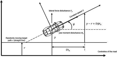
Figure 1 illustrates the steering control task. The vehicle travels at constant forward speed $U$ and has lateral displacement $y$ and heading angle $\psi$. Angles are assumed to be small. The driver steers to follow a straight target path that has randomly changing lateral displacement $r$, which means that the driver does not have any preview of the future target displacement. A similar steering task was employed in [12]. The absence of preview ensures that the driver’s control action is entirely feedback in nature (no feedforward) and thus the task emphasises the role of steering torque feedback in providing state information to the driver. Although there is no preview of the target path displacement, account is taken of the possibility that the driver aims to minimise the lateral distance between the target path and the longitudinal axis of the vehicle at some distance in front of (or behind) the centre of mass of the vehicle. The distance is parameterised by time shift $t_s$ multiplied by the vehicle speed $U$. The driver is also required to compensate for random disturbances acting on the vehicle: torque disturbance $T_d$ acting on the steering column, and lateral force $F_y$ and yaw moment $M_z$ acting on the centre of mass of the vehicle (although $F_y$ and $M_z$ were set to zero for the experiments reported in this paper). The steering task is designed to put the vehicle in the ‘on-centre’ regime, associated with travelling in a nominally straight line and with lateral acceleration no greater than about 2ms⁻². The on-centre regime is experienced by most drivers most of the time and is important in the subjective assessment of steering torque feedback.

Figure 1. On-centre steering control task. The driver steers the vehicle to follow a straight target path that has randomly changing lateral displacement $r$. The driver must also reject random disturbances $T_d$, $F_y$ and $M_z$ acting on the steering-vehicle system. Angles are assumed to be small.

A block diagram of the driver-steering-vehicle model is shown in Figure 2. The plant is linear and comprises the vehicle and steering system, including the driver's muscles. Plant disturbances are white noises $w_F$, $w_M$, $w_T$ and $w_r$(with corresponding standard deviations $W_F,W_M,W_T,W_r$) that are filtered in the plant to give the four disturbances introduced in the preceding paragraph. Plant outputs $\mathit{z}$are the human sensory measurements to which sensory measurement white noise $\mathit{v}$ is added to give noisy measurements ${\mathit{z}}_{\nu }$. The plant is actuated by a muscle activation signal $u$, comprising cognitive control $\alpha$, stretch reflex ${\alpha }_{\mathrm{rd}}$ and neuromuscular process white noise $w$ (with standard deviation $W$). The stretch reflex is a relatively fast local feedback control of muscle length ${\theta }_a$ (referred to angle about the steering column axis). The stretch reflex transfer function is a simple gain $k_r$ that generates signal ${\alpha }_r$, followed by a delay ${\tau }_r$, acting on the difference between the predicted muscle length $\gamma$ and the noise-free sensed muscle length ${\theta }_a$.

Figure 2. Block diagram of the linear driver-steering-vehicle model. The plant comprises the vehicle and steering system, including the driver's steering muscles. Plant disturbances are white noises $w_F$, $w_M$, $w_T$ and $w_r$ that are filtered in the plant. Plant outputs $\mathit{z}$ are perturbed with measurement noise $v$. The plant is actuated by a muscle activation signal u, comprising cognitive LQR control $\alpha$, reflex action ${\alpha }_{\mathrm{rd}}$ and process noise $w$. The Kalman filter receives an efference copy from the LQR. The Kalman filter generates estimates ${\mathit{x}}_{\mathit{e}}$ of the plant states for use by the LQR.

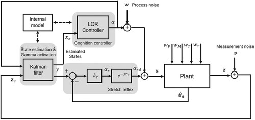
The driver’s control strategy follows the linear quadratic Gaussian (LQG) framework, combining a linear quadratic regulator (LQR) with a Kalman filter to give optimal control action $\alpha$ and state estimates ${\mathit{x}}_{\mathit{e}}$. The Kalman filter receives an efference copy from the LQR. The Kalman filter also generates the predicted muscle length $\gamma$. The LQR acts to minimise a quadratic cost function: (1) $\begin{array}{r}J=\sum _{k=0}^{k=\mathrm{\infty }}{q}_e[y(k)-r(k)+\psi (k)U{t}_s{]}^2+\alpha (k{)}^2\end{array}$(1) where $q_e$ is a weighting that penalises lateral displacement of the vehicle from the target at a distance $U{t}_s$ ahead of the centre of mass of the vehicle and $k$ is a discrete time step index. The cognitive control signal $\alpha$ has unity weighting. The Kalman filter is parameterised by the process noise variances and measurement noise variances. The LQR and Kalman filter use an exact ‘internal’ model of the plant[12].

Figure 3 shows the plant in more detail. The three main blocks are: muscle activation dynamics ($H_a$) represented as two first-order lags in series to generate muscle torque $T_a$; muscle and steering dynamics ($H_{\mathrm{ms}}$) described in the next paragraph; and vehicle dynamics ($H_v$) represented by the well-known two-degree-of-freedom single-track model with linear tyres. It could be argued that the vehicle model should be more complicated to better represent the dynamics of a real vehicle, but for the purpose of the present research it is important that the human test subject can learn an accurate internal model of the vehicle dynamics, which has been shown to be possible for a linear two-degree-of-freedom single-track model [12]. Also shown in Figure 3 are the disturbance filters ($H_{\mathrm{fT}}$, $H_{\mathrm{fF}}$, $H_{\mathrm{fM}}$ and $H_{\mathrm{fr}}$). Mechanical coupling between the vehicle dynamics and the steering dynamics is provided by the column angle ${\theta }_c$ and self-aligning moment $T_w/G$ signals ($G$ is defined in the next paragraph). There are three sensory measurements: visually-sensed vehicle lateral displacement relative to the target path $e=y-r$; visually-sensed vehicle yaw angle $\psi$; and proprioceptively-sensed muscle length ${\theta }_a$ referred to the steering column axis. The three sensory measurements are subject to time delays, ${\tau }_{\mathrm{vi}}$ for the visual measurements and ${\tau }_{\mathrm{\theta a}}$ for the muscle length, resulting in perceived signals $e_d$, ${\psi }_d$ and ${\theta }_{\mathrm{ad}}$. The standard deviations of the uncorrelated noises subsequently added to the three sensory measurements are $V_e,V_{\psi },V_{\mathrm{\theta a}}$. Steering torque is assumed to be perceived primarily via the cognitive muscle activation signal $\alpha$, consistent with previous experimental research [14]; no other potentially torque-sensing organs such as skin receptors or Golgi tendons are included in the model, in order to minimise the risk of overfitting and to avoid the difficulties noted in [9]. There is no vestibular feedback of vehicle motion in the model, to focus attention on the steering torque feedback and to minimise the number of parameters and thus the risk of overfitting. The absence of vestibular feedback in the model meant that the experiments could be performed in a fixed-base driving simulator; this is discussed further in Section 3 and in [17,18]. In [12,16] a complementary approach was taken: the model included vestibular feedback but no steering torque feedback, and a moving base simulator was used. Identifying and validating a model incorporating both vestibular feedback and steering torque feedback is future work.

Figure 3. Block diagram of the plant, comprising muscle activation dynamics $H_a$, muscle and steering dynamics $H_{\mathrm{ms}}$, vehicle dynamics $H_v$, human sensory measurement delays and plant disturbance filters $H_{\mathrm{fT}}$, $H_{\mathrm{fF}}$, $H_{\mathrm{fM}}$ and $H_{\mathrm{fr}}$.

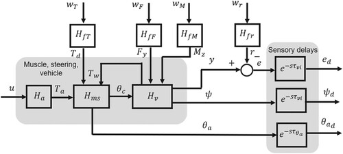
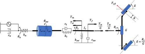
Figure 4 shows the muscle and steering dynamics $H_{\mathrm{ms}}$. Lateral force at the front axle $F_{\mathrm{yf}}$ is multiplied by the trail distance d to obtain the self-aligning steering torque $T_w$. Dividing by the steering gear ratio ($G={\theta }_c/\delta$ where ${\theta }_c$ is the column (pinion) angle and $\delta$ is the front wheel steer angle) gives the pinion torque $T_w/G$. Inertia $I_c$ represents the steering column and the roadwheels (referred to the column axis). Passive stiffness $k_{\mathrm{sw}}$ and damping $c_{\mathrm{sw}}$ oppose column rotation; the passive stiffness represents the self-centring torque arising from king-pin inclination. Power steering assistance torque $T_m$ and friction torque $T_f$ can be applied to the column (both set to zero for the experiments described in the present paper, for simplification), while torque disturbances are applied as $T_d$. The spring $k_t$ and damper $c_t$ represent a torsion bar between the steering column and the handwheel. The inertias of the handwheel $I_{\mathrm{sw}}$ and the driver's arms $I_{\mathrm{arm}}$ are assumed to be rigidly coupled at the contact between the hand and the handwheel, with the handwheel steering angle denoted as ${\theta }_{\mathrm{sw}}$. The muscle dynamics are described by a simplified Hill muscle model [21], comprising activation torque $T_a$, tendon stiffness $k_a$ and muscle damping $c_a$. The muscle length sensed by the muscle spindles is ${\theta }_a$.

Figure 4. Muscle and steering system model with steering column torque disturbance. All springs and dampers act in torsion, aligned with the steering column axis.

In total there are about forty parameters in the driver-steering-vehicle model. The parameter values of the vehicle correspond to a mid-size passenger car. The values of the remaining parameters are either: (i) defined by the operating conditions; or (ii) estimated from the published literature (for details see [7,8]); or (iii) identified from driving simulator experiments described in the present paper. The eleven parameters to be identified from the driving simulator experiments are:

• Neuromuscular parameters: muscle damping $c_a$, arm inertia $I_{\mathrm{arm}}$, reflex gain $k_r$.

• Cognitive parameters: process noise standard deviation $W$, measurement noise standard deviations $V_e$, $V_{\psi }$, $V_{{\theta }_a}$, path-following error weight $q_e$, time shift $t_s$.

• Sensory delays: visual delay ${\tau }_{\mathrm{vi}}$, muscle angle sensory delay ${\tau }_{{\theta }_a}$.

3. Driving simulator experiments

3.1. Driving simulator

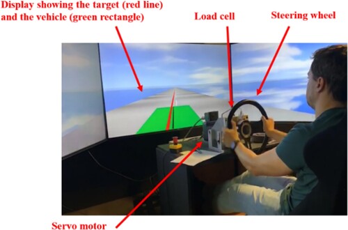
The fixed-base driving simulator is shown in Figure 5. It consists of: three 65-inch displays providing the driver with 138 degrees field of view; a host computer providing overall control of the simulator; a target computer running the real-time steering-vehicle system model; a graphics computer running the virtual reality world; a handwheel driven by a servo motor; an optical encoder measuring the handwheel angle; and a six-axis load cell measuring the forces and torques applied by the driver to the handwheel. The human test driver is presented with the view that would be seen by someone steering the vehicle remotely while following the vehicle a constant 7 m behind the centre of mass of the vehicle. The driver is assumed to travel in a straight line while the target path (red line) and vehicle (green rectangle) move laterally. The reason for this arrangement is to ensure that there are no conflicts between the driver’s visual and vestibular sensory measurements, which could lead to nausea and unrealistic use of the sensory measurements by the driver [16].

Figure 5. Driving simulator with test subject.

3.2. Steering control task

The steering control tasks are described in the beginning of section 2. Three trials were designed as shown in Table 1. Trial 1 consisted of random steering column torque disturbance only, a stationary target path and zero trail distance. This trial was designed to provide rich data for identifying the neuromuscular parameters of the driver model. In trial 2 the target path had random lateral displacement but there were no other external disturbances, and the trail distance was zero. Trial 3 was the same as trial 2 except that the trail distance was non-zero, thereby introducing a component of steering torque from the lateral force at the front axle. The vehicle speed U in all trials was 16.7 m/s (60 km/hour). This speed was chosen in combination with the disturbance spectral densities described in the next paragraph to provide sufficient signal amplitudes without tiring the test subjects.

Table 1. Experimental conditions for each trail.

	Standard deviation of disturbances
Trial	$W_r(\text{m})$	$W_F(\text{N})$	$W_M(\text{Nm})$	$W_T(\text{Nm})$	Trail distance $d(\text{mm})$
1	$0$	$0$	$0$	$4$	$0$
2	$8$	$0$	$0$	$0$	$0$
3	$8$	$0$	$0$	$0$	$59$

The randomly moving target line and the column torque disturbance were generated using filtered Gaussian white noise. White noise signals $w_F$ and $w_r$ were generated in discrete time. The standard deviations $W_F,W_r$ of these signals were tuned during preliminary testing to give a suitable trade-off between achieving a high signal-to-noise ratio and a comfortable experience for the test subjects. The cut-off frequency $f_{\mathrm{cT}}$ of the low-pass filter $H_{\mathrm{fT}}$ for the column torque disturbance was set to 10 Hz, to ensure that the human subjects were not excited significantly beyond the frequencies of interest. The filter $H_{\mathrm{fr}}$ for generating the target path was implemented as a band-pass filter, following the practice in [12]. The filter had 40 dB/decade slope at high and low frequencies, with upper and lower cut-off frequencies of 1 and 0.05 rad/s.

3.3. Experiment procedure and trials

Thirteen test subjects aged from 21 to 30 were employed in the experiment. Because reaction times and sensory threshold have been found to increase with age [22,23], test subjects were chosen within a narrow range of age to allow combining of datasets from different drivers, and therefore benefit model identification by increasing the signal-to-noise ratio. All test subjects were professional vehicle dynamics engineers or experienced drivers.

Before performing the experiments, a ten-minute training session consisting of practice runs of the trials was conducted to reduce the learning effect and to help the test subjects become familiar with the driving simulator, the steering task, the different disturbances, and the steering-vehicle system dynamic characteristics. The three trials were presented to every driver. Each driver was presented with the same time histories of random disturbance, to allow subsequent averaging of response time histories across drivers. The drivers were not told anything about the specific conditions of each trial. Measured data was collected for five minutes for each trial. The data recorded in the first minute of each trial was disregarded in the subsequent analysis to reduce the influence of possible transient behaviour at the start of each trial. In trials 2 and 3, the drivers were asked to provide subjective assessment of the steering torque feedback for each trial.

Ethical approval of the experiment was obtained from the Research Ethics Committee, Department of Engineering, University of Cambridge on 6 December 2016. All subjects provided informed consent by means of a Participant Information Sheet and a signed Consent Form.

3.4. Data analysis

Statistical analysis of the values of RMS path-following error and RMS handwheel angle of each test subject in each trial was conducted to determine if there were significant differences in the data between trials 2 and 3. Both trials involved a randomly moving target path, but only trial 3 had a component of steering torque due to lateral force at the front axle. For details of the analysis see [17]. The analysis showed that the addition of steering torque feedback in trial 3 led to the test subjects following the target path more accurately (RMS path error reduced from 0.401 m to 0.370 m) and with smaller steering wheel angle inputs (RMS angle reduced from 0.457 rad to 0.410 rad). The subjective assessments by each test subject were also analysed. The results confirmed that the drivers preferred the presence of steering torque feedback in trial 3.

4. Driver model identification

A procedure similar to that employed in [12] was used to identify values of the eleven parameters of the driver model specified in Section 2 by searching for the best fit to the handwheel angle time histories measured in the driving simulator experiments.

The identification procedure consists of two stages: (i) a Box-Jenkins model identification to find general polynomial transfer functions, giving an upper bound on the prediction accuracy achievable by a linear parametric model; and (ii) parametric identification to find the unknown parameter values of the driver model. The identification procedure is applied separately for each driver, and to ‘averaged data’ generated by averaging the measured handwheel angle time series of all the individual drivers. If it is assumed that the drivers use similar steering control strategies, a set of more reliable parameter values can be found using averaged data because the signal to noise ratio is improved. As mentioned in Section 3, the first minute of each trial is disregarded. The next three minutes of data are used for identification and the final minute of data is used for validation, that is, to check for over-fitting.

4.1. Box-Jenkins identification

The Box-Jenkins model is a set of polynomial transfer functions between each of the inputs (steering column torque disturbance $T_d$ and target lateral position $r$) and the output (handwheel angle ${\theta }_{\mathrm{sw}}$) [24,25]. There is also an output noise model. The structure of the Box-Jenkins model is: (2) $\begin{array}{r}{\theta }_{\mathrm{sw}}(k)=\frac{B_{T_d}(q)}{F_{T_d}(q)}{T}_d(k-n_2)+\frac{B_r(q)}{F_r(q)}r(k-n_3)+\frac{C_{\mathrm{sw}}(q)}{D_{\mathrm{sw}}(q)}{w}_{\mathrm{sw}}(k)\end{array}$(2) where: variables $B_{T_d}$, $B_r$, $F_{T_d}$, $F_r$, $C_{\mathrm{sw}}$ and $D_{\mathrm{sw}}$ are fifth-order polynomials expressed in the time-shift operator $q^{-1}$; k is discrete time step index; $n_2$ and $n_3$ are time step delays. A genetic algorithm was used to find the values of these delays prior to identifying the transfer functions. A separate model was identified for each of the three trials.

4.2. Parametric identification

The parametric driver model is identified indirectly by minimising the prediction error of the closed-loop driver-vehicle model [12]. The mean-square difference of the simulated and measured handwheel angles $\text{E}[{({\theta }_{\mathrm{sw}(\mathrm{sim})}-{\theta }_{\mathrm{sw}(\exp )})}^2]$ is minimised to find the optimum set of values for the eleven unknown parameters. There are two primary sources contributing to the prediction error. The first is modelling error, which is assumed to be negligible. The second is the driver’s random neural noise (process and measurement), which cannot be eliminated. However, bias may be introduced to the identification if the noise in the driver's measured handwheel angle is not white. To address this problem, a weighted prediction error $\epsilon$, as defined in (3), is minimised in the identification, as suggested by Ljung [24]. (3) $\begin{array}{r}\epsilon (s)=\frac{1}{H_n(s)}{\left(\frac{2\pi f_c}{s+2\pi f_c}\right)}^2({\theta }_{\mathrm{sw}(\mathrm{sim})}(s)-{\theta }_{\mathrm{sw}(\exp )}(s))\end{array}$(3) The weighted prediction error $\epsilon$ is obtained by filtering by the inverse of the noise model $H_n(s)$ found in the Box-Jenkins identification (2). However, this will result in an increased prediction error amplitude at frequencies in excess of the human driver’s normal operating range. Therefore a low-pass filter is also included to reduce the high-frequency components of the weighted prediction error. The cut-off frequency $f_c$ of the low-pass filter is set to 5 Hz for trial 1 and 3 Hz for trials 2 and 3. The higher cut-off frequency for trial 1 reflects the near-direct application of torque disturbance to the driver's arms and consequent higher-frequency responses in that trial.

The minimisation problem may have local minima. First, a genetic algorithm [12,26] is used with 100 random combinations of parameter values as starting points to find the global minimum. A Newton method (Matlab ‘fmincon’ with SQP) is then used to refine the minimum.

Initially, single sets of parameter values are identified for each driver and for the averaged driver using the data from all three trials simultaneously, using a four-step procedure as shown in Table 2. Multiple steps are needed to minimise the risk of over-fitting that arises from identifying a relatively large number of parameters. In step 1, all the parameters are identified across all three trials. The identified value of the process noise standard deviation $W$ is then adjusted to make the simulated driver noise standard deviation equal to the standard deviation of the prediction error, following the procedure in [12]. In step 2, the process noise standard deviation $W$ is held constant while the remaining parameters are identified to fit the results of all three trials once more. In step 3, the three neuromuscular parameters are identified using all three trials, while the other parameters are fixed at the values identified in step 2. In step 4, the process noise standard deviation $W$ and the cognitive controller time shift $t_s$ are kept constant at the values found in step 2, the neuromuscular parameters are kept constant at the values found in step 3, and the remaining six parameters are identified across all three trials. For the averaged driver, the process noise standard deviation $W$ is also scaled to match the standard deviation of the measured noise found in the data after step 1 and is then fixed in the subsequent steps. The average of the adjusted values of $W$ for each of the thirteen drivers could also be used for the averaged driver after step 1. The difference between the two approaches to identify the process noise standard deviation $W$ for the averaged driver is discussed in Section 4.4.

Table 2. Conditions for each step of the parametric identification procedure to find a single set of parameter values for each driver (or the averaged driver) across all three trials. $\times$ indicates parameters to be identified at each step.

		Neuromuscular parameters			Cognitive parameters						Sensory delays
Step	Trials	$c_a$	$I_{\mathrm{arm}}$	$k_r$	$W$	$V_e$	$V_{\psi }$	$V_{{\theta }_a}$	$t_s$	$q_e$	${\tau }_{\mathrm{vi}}$	${\tau }_{{\theta }_a}$
1	1, 2, 3	$\times$	$\times$	$\times$	$\times$	$\times$	$\times$	$\times$	$\times$	$\times$	$\times$	$\times$
2	1, 2, 3	$\times$	$\times$	$\times$		$\times$	$\times$	$\times$	$\times$	$\times$	$\times$	$\times$
3	1, 2, 3	$\times$	$\times$	$\times$
4	1, 2, 3					$\times$	$\times$	$\times$		$\times$	$\times$	$\times$

After a single set of parameter values fitting all three trials is found for each driver and the averaged driver, separate sets of parameter values are identified for each combination of driver and trial. The identification procedure starts with the single set of parameters previously identified for each driver. Then for each trial: (i) the process noise $W$ is scaled; (ii) the arm inertia $I_{\mathrm{arm}}$ and the cognitive controller time shift $t_s$ are fixed at the values previously identified for each driver; (iii) the remaining parameters are identified. Separate parameter sets for each driver and trial combination are likely to give better agreement between measurement and simulation but are perhaps less useful as a predictive tool, unless it is also determined how the parameter values depend on the properties of the trial. The risk of over-fitting is also increased, due to the smaller amount of data used for identification of each parameter set.

4.3. Agreement between model and measurements

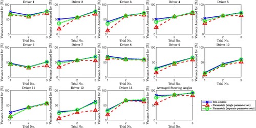
The goodness of the fit of the identified model to the experimental data is quantified using the ‘variance accounted for’ (VAF), which is the percentage of the variance in the measured handwheel angle ${\theta }_{\mathrm{sw}(\exp )}$ explained by the modelled handwheel angle ${\theta }_{\mathrm{sw}(\mathrm{sim})}$, and is given by: (4) $\begin{array}{r}\mathrm{VAF}=\left(1-\frac{{\sum }_k{\{{\theta }_{\mathrm{sw}(\mathrm{sim})}(k)-{\theta }_{\mathrm{sw}(\exp )}(k)\}}^2}{{\sum }_k{\{{\theta }_{\mathrm{sw}(\exp )}(k)\}}^2}\right)\times 100\text{\%}\text{. }\end{array}$(4) where $k$ is the time-step index. Figure 6 shows the VAF values of the identified models for each combination of driver and trial. As expected, the VAFs are largest for the Box-Jenkins model. The VAFs for the separate parameter sets are quite close or even equal to the VAFs for the Box-Jenkins model, indicating that the parametric driver model structure can explain the drivers’ linear steering control behaviour quite well. The VAFs for the single parameter sets are close to the VAFs for the separate parameter sets, indicating that one model is able to provide a good approximation to the measured steering response of a driver across the three trials. There are some differences within and between drivers in terms the VAFs achieved for the trials. For example, driver 1 generally achieves high VAFs in all three trials, whereas driver 11's VAFs for trial 1 are very low, but their VAFs for trails 2 and 3 are close to those achieved by other drivers. The VAFs of drivers 6, 10, 11, 12 are generally lower than for the other drivers. It is difficult to determine specific reasons for these differences. Lower VAFs may be due to: high process or measurement noise; nonlinear or inconsistent driver behaviour; or insufficient model complexity to represent the driver's steering strategy. For the averaged driver, the mean VAF across the three trials is 75% for the single set of parameter values, and 84% for the separate parameter sets. The VAFs for the averaged driver are thought to be higher than for individual drivers because time-series averaging reduces the contribution of noise to the prediction error. These VAF values are higher than those obtained by Nash and Cole [12] for their model of steering control with vestibular feedback, but they only had data from five test subjects.

Figure 6. Agreement between simulated and measured handwheel angle, quantified as ‘variance accounted for’ (VAF). Blue crosses are for the Box-Jenkins model. Red triangles are VAFs achieved with a single set of parameter values identified for each driver across all three trials. Green circles are VAFs achieved with separate sets of parameter values identified for each driver/trial combination.

4.4. Identified parameter values

The single parameter sets identified for each driver across all three trials are shown in Figure 7 and are broadly similar between the different drivers, suggesting that the drivers had similar properties and were using similar control strategies. The parameter values found using the averaged driver all fall within the range of the parameter values found for the individual drivers, suggesting that the averaged data might be a valid representation of a typical driver’s steering control behaviour.

Figure 7. Identified single parameter sets fitting all three trials for the individual drivers (crosses) and the averaged data (solid horizontal lines). The average of the values of $W$ for the thirteen drivers, with the corresponding identified values of $V_e$, $V_{\psi }$ and $V_{{\theta }_a}$ for the averaged data are shown by the red dashed horizontal lines.

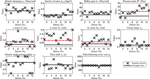
The arm inertia $I_{\mathrm{arm}}$ and the sensory delays ${\tau }_{\mathrm{vi}}$ and ${\tau }_{{\theta }_a}$ relate to each driver’s internal physical properties, while the muscle damping $c_a$ and the stretch reflex gain $k_r$ are mainly determined by the muscle states the drivers used when they performed the experiments. It is likely that drivers with larger values of $c_a$ and $k_r$ tensed their muscles more than the other drivers during the experiments.

The path-following error cost $q_e$ indicates the trade-off between the steering effort and the path following accuracy, while the cognitive controller time shift $t_s$ describes which part of the vehicle the driver aims to align with the target path; these two parameters are choices made by the human drivers during the experiments instead of being determined by physical properties. The identified values of $q_e$ for most of the drivers hit the upper bound constraint in the optimisation of 1000. This is because $q_e$ was significantly larger for trial 1 than for trials 2 and 3. The constraint was necessary to avoid biasing the other parameter values when identifying a single parameter set across all three trials.

The noise parameters $W$, $V_e$, $V_{\psi }$ and $V_{{\theta }_a}$ appear in two places in the model: as standard deviations of the added process and measurement noise; and as parameters of the state estimator. Drivers 6, 10, 11 and 12, who exhibited lower VAF values than the other drivers in Figure 6, are found in Figure 7 to have relatively high values of process or measurement noise. Driver 6 has a high value of $V_e$; driver 10 has high values of $V_{\psi }$ and $W$; and drivers 11 and 12 have high values of process noise $W$. As expected, the value of process noise standard deviation $W$ identified from the averaged data (black solid line) is smaller than the average of the values of $W$ identified for each of the thirteen drivers (red dashed line), because driver noise is reduced by averaging the handwheel angle response of the thirteen drivers.

The separate parameter sets identified for each driver and each trial are not shown due to insufficient space but can be seen in [17]. The identified values of muscle damping c_a and stretch reflex gain k_r in trial 1 are larger compared with those in trials 2 and 3. This is because tensing (co-contracting) the arm muscles is an effective control strategy in the presence of high-frequency steering column disturbances, but is not so effective when the disturbance is a lower frequency target path. In trial 1 the controller cost function weight on path-following error q_e is an order of magnitude larger than in trials 2 and 3, indicating a significant difference in the effect of column torque disturbance and target path disturbance.

4.5. Measured and modelled driver noise

It is of interest to determine if there is a relationship between the standard deviations of the process noise $W$ and the muscle activation torque $T_a$. Because the muscle activation torque is not directly measured in the experiments the signal is estimated as $T_{a(\exp )}$ using the measured data and the identified parametric driver model, see [17] for details.

Figure 8(a) shows the values of process noise W against the values of RMS estimated muscle activation torque $T_{a(\exp )}$ in the experiment. There is a clear linear relationship between these two variables, indicating that the process noise is signal dependent. The signal-to-noise ratio (SNR), defined here as the ratio of RMS estimated muscle activation torque $T_{a(\exp )}$ to process noise standard deviation W, is plotted for each driver in Figure 8(b). The values of SNR are broadly similar between different drivers, and the average SNR over all thirteen drivers is 0.47, which is comparable to the value obtained by Nash and Cole [12].

Figure 8. Investigation into signal-dependent driver noise. In (a), the identified process noise standard deviation W is compared with the RMS estimated muscle activation torque $T_{a(\exp )}$ of the experiment. In (b), the SNRs for the individual drivers (crosses) are compared and the average SNR (solid horizontal line) over all the drivers is calculated. In (c), identified measurement noise standard deviations are compared with the corresponding RMS signal amplitudes for path-following error, heading angle, and muscle angle. Straight lines passing through the origin are plotted to assess the existence of a constant SNR.

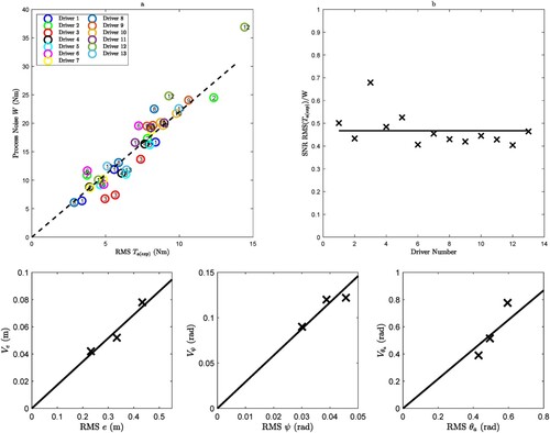
To investigate the signal to noise ratio of the sensory measurements, two additional trials were performed by drivers 9 to 13, for which the properties of the steering-vehicle dynamics were identical to those in trial 3 but the standard deviation of the target path lateral displacement was varied above and below the value used in trial 3. The identification procedure described in Section 4.2 was then run for the averaged data of the drivers. Figure 8(c) shows the identified measurement noise standard deviations $V_e$, $V_{\psi }$ and $V_{{\theta }_a}$ for the three trials (trial 3 and the two additional trials) against RMS values of the corresponding signals. The linear trends indicate that sensory measurement noise is also signal-dependent, consistent with findings in [16]. It should be noted there is also expected to be a sensory measurement threshold below which signals cannot be detected.

5. Driver model with constant signal to noise ratio

Before proceeding to validate the identified model using the final minute of the measured data, one more round of parameter identification is performed. In light of the constant SNR behaviour identified in Section 4, the process and measurement noise are parameterised as SNRs: (5) $\begin{array}{r}\mathrm{SN}{R}_W=\frac{\text{RMS}(T_a)}{W},\mathrm{SN}{R}_e=\frac{\text{RMS}(e)}{V_e},\mathrm{SN}{R}_{\psi }=\frac{\text{RMS}(\psi )}{V_{\psi }}\text{and}\mathrm{SN}{R}_{{\theta }_a}=\frac{\text{RMS}({\theta }_a)}{V_{{\theta }_a}}.\end{array}$(5) Because trial 1 is less typical of normal driving activity, single sets of parameter values for each driver and the average driver are identified from the combined data of trials 2 and 3 only. Details of the identification steps are given in [17]. The results are shown in Figure 9. Overall, the identified parameter values, especially the process and measurement noise SNRs, are similar between different drivers, and the values found using the averaged data all fall within the range of the parameter values found for the individual drivers.

Figure 9. Identified single parameter sets fitting the linear trials 2 and 3 for the individual drivers (crosses) and the averaged data (solid horizontal lines). The average of the scaled values of $\mathrm{SN}{R}_W$ over the thirteen drivers, with the corresponding identified values of $\mathrm{SN}{R}_e$,$\mathrm{SN}{R}_{\psi }$ and $\mathrm{SN}{R}_{{\theta }_a}$ for the averaged data are shown by the red dashed horizontal lines.

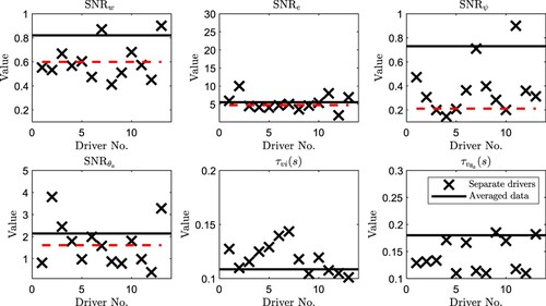
The identified parameter values for the averaged driver are given in Table 3. The identified values of neuromuscular parameters are compared with those obtained by Hoult [27], who proposed a neuromuscular model for simulating driver steering torque and found ranges of values of the muscle damping, the arm inertia, and the stretch reflex for muscles with different states through experiments. It is seen that the identified stretch reflex gain $k_r$ is within the range found by Hoult, while the identified muscle damping $c_a$ and arm inertia $I_{\mathrm{arm}}$ are relatively larger than the corresponding values found by Hoult. However, the muscle model used in Hoult’s studies is slightly different from Hill’s muscle model [21]. In addition, the values found by Hoult are identified through passive conditions and therefore, may not be applicable for an active steering control task. By taking these factors into account, the difference in the identified neuromuscular parameter values is plausible. Nash and Cole [16] found a set of process and measurement noise SNRs in the study of human sensory feedback in car driving. The identified values of process noise $\mathrm{SN}{R}_W$ and visual vehicle yaw angle measurement noise $\mathrm{SN}{R}_{\psi }$ in the present study are comparable with the those found by Nash and Cole, while the identified value of visual path-following error measurement noise $\mathrm{SN}{R}_e$ is much greater than the value found by Nash and Cole. However, the selected sensory measurement channels in the model developed by Nash and Cole are not directly comparable with the ones used in the present study, which may influence the human driver’s weighting on each sensory measurement in the state estimator. The identified sensory delays are all within the ranges reported in [28].

Table 3. Mean and standard deviation of the parameter values identified for the drivers across trials 2 and 3. Identified parameter values are compared with estimates from the published literature.

Parameter	$c_a$	$I_{\mathrm{arm}}$	$k_r$	$\mathrm{SN}{R}_W$	$\mathrm{SN}{R}_e$
Units	$\text{Nms}/\text{rad}$	$\text{kg}{\text{m}}^2$	$\text{Nm}/\text{rad}$
Mean	$3.37$	$0.0973$	$24.9$	$0.600$	$4.75$
Standard deviation	$0.910$	$0.0375$	$7.00$	$0.154$	$1.99$
Literature	$0\text{ to }1.25$	$0.0286\text{ to }0.0446$	$0\text{ to }50.0$	$0.57$	$0.901$
Source	[27]	[27]	[27]	[16]	[16]
Parameter	$\mathrm{SN}{R}_{\psi }$	$\mathrm{SN}{R}_{{\theta }_a}$	${\tau }_{\mathrm{vi}}$	${\tau }_{{\theta }_a}$	$t_s$
Units			$\text{s}$	$\text{s}$	$\text{s}$
Mean	$0.210$	$1.61$	$0.109$	$0.180$	$0.023$
Standard deviation	$0.228$	$0.995$	$0.0133$	$0.0303$	$0.308$
Literature	$0.415$	$-$	$0.10\text{ to }0.56$	$0.034$	$-$
Source	[16]		[28]	[28]

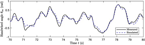
The average VAF values across the two trials for each driver and for the averaged driver (driver 14) are presented in Figure 10 (solid lines). Also shown are the corresponding VAF values calculated from the validation data (last minute of each trial). In general, the VAF values in the validation data are similar to those in the identification data, indicating that the driver model is not overfitted. Drivers 6, 10, 11, 12 again show the lowest VAF values, although there is no obvious correlation with the identified parameter values in Figure 9. In comparison to the process and measurement noise parameters in Figure 7, the SNR parameters in Figure 9 do not necessarily scale with noise variance. The VAF value of the parametric model calculated from the validation data for the averaged driver (driver 14 in Figure 10) over the two trials was 86.6%. Typical time histories of handwheel angle for the averaged driver in trial 3, measured and simulated, are shown in Figure 11.

Figure 10. Validation of the parametric driver model with SNRs for each driver including the averaged driver (Driver 14). The VAFs obtained from the identification data are represented by the triangles on black solid lines for the Box-Jenkins model and the red crosses on red solid lines for the parametric model. The VAFs obtained from the validation data and the parametric model are represented by the black crosses on the dashed lines.

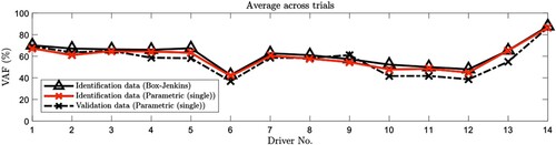
Figure 11. Typical time histories of handwheel angle for the averaged driver in trial 3, measured and simulated.

6. Conclusion

The published literature in the field of driver models with steering torque feedback was reviewed. It was found that several studies had attempted to account for the effect of steering torque feedback, but there was inconsistency in which neural and biomechanical mechanisms were included in the models. Based on the findings of the literature survey a new linear parametric driver-steering-vehicle model was proposed incorporating: neuromuscular dynamics including stretch reflex; proprioceptive (muscle stretch) and visual sensory dynamics, including measurement noise; a state estimator including efference copy; steering torque perception via the efference copy; and an internal model.

A series of path-following experiments with thirteen test subjects was performed on a fixed-base driving simulator. Each test subject performed three different trials in the ‘on-centre’ regime of operation. The addition of steering torque feedback from the lateral tyre force was found to reduce RMS path following error from 0.401 m to 0.370 m and RMS handwheel angle from 0.457 rad to 0.410 rad. The driving simulator data was used to identify a Box-Jenkins linear model, which accounted for 90% of the variance of the measured handwheel angle time series averaged over the thirteen test subjects. The values of eleven parameters of the parametric model were identified from the driving simulator data. The fit of the identified model to the experimental results approached the upper bound limit given by the Box-Jenkins model. The identified process noise standard deviation was found to be linearly dependent on RMS muscle activation torque, and this signal-dependent behaviour was also present in the identified measurement noise.

The model was re-identified for two of the three trials using signal to noise ratios as parameters in place of noise standard deviations. The averaged VAF value over the two trials was 86.6% of the variance of the measured handwheel angle averaged over the thirteen test subjects. Prediction accuracy close to that of the Box-Jenkins model, and identified parameter values that were physically plausible, give confidence that the model is suitable for further work on understanding the driver’s objective and subjective response to steering torque feedback. Further work could include: extending the model to account for nonlinearities in the steering mechanism such as column friction torque; investigating the relationship of subjective assessment to prediction error of the internal model; and extending the model with target path preview and vestibular motion sensing.

Acknowledgement

The financial and technical contributions of Toyota Motor Europe (RG88816) are gratefully acknowledged.

For the purpose of open access, the author has applied a Creative Commons Attribution (CC BY) licence to any Author Accepted Manuscript version arising from this submission.

Disclosure statement

No potential conflict of interest was reported by the author(s).

References

- Harrer M, Pfeffer P, Braess HH. Steering-feel, interaction between driver and car. In: Harrer M, Pfeffer P, editor. Steering handbook. Cham: Springer; 2017. doi:10.1007/978-3-319-05449-0_7
- Gil Gomez GL, Nybacka M, Bakker E, et al. Correlations of subjective assessments and objective metrics for vehicle handling and steering: a walk through history. Int J Veh Des. 2016;72(1):17–67. doi:10.1504/IJVD.2016.079191
- Ketzmerick E, Zösch P, Abel H, et al. A validated Set of objective steering feel parameters focusing on non-redundancy and robustness. In: Bargende M, Reuss HC, Wagner A, editor. Internationales stuttgarter symposium. proceedings. Wiesbaden: Springer Vieweg; 2022. doi:10.1007/978-3-658-37011-4_34
- Sharp RS. Some contemporary problems in road vehicle dynamics. Proc Inst Mech Eng Pt C J Mechan Eng. Jan. 2000;214(1):137–148.
- Cole DJ. Occupant–vehicle dynamics and the role of the internal model. Veh Syst Dyn. 2018;56(5):661–688. doi:10.1080/00423114.2017.1398342
- Pick AJ, Cole DJ. A mathematical model of driver steering control including neuromuscular dynamics. J Dyn Syst Meas Control Trans ASME. 2008;130(3):031004. doi:10.1115/1.2837452
- Cole DJ. A path-following driver-vehicle model with neuromuscular dynamics, including measured and simulated responses to a step in steering angle overlay. Veh Syst Dyn. 2012;50(4):573–596. doi:10.1080/00423114.2011.606370
- Katzourakis D, Droogendijk C, Abbink D, et al. Driver model with visual and neuromuscular feedback for objective assessment of automotive steering systems. In: M Best, editor. Proceedings of the 10th international symposium on advanced vehicle control. AVEC10. The 10th International Symposium on Advanced Vehicle Control. Loughborough; Aug 2010. p. 381–386.
- Mugge W, Abbink DA, Schouten AC, et al. Force control in the absence of visual and tactile feedback. Exp Brain Res. 2013;224:635–645. doi:10.1007/s00221-012-3341-z
- Mars F, Saleh L, Chevrel P, et al. Modeling the visual and motor control of steering with an eye to shared-control automation. Proc Hum Factors Ergon Soc Annu Meet. 2011;55(1):1422–1426. doi:10.1177/1071181311551296
- Zhao Y, Chevrel P, Claveau F, et al. Towards a driver model to clarify cooperation between drivers and haptic guidance systems. 2020 IEEE international conference on systems, Man, and cybernetics (SMC); Toronto, ON, Canada, 2020, pp. 1731–1737, doi:10.1109/SMC42975.2020.9283101
- Nash CJ, Cole DJ. Identification and validation of a driver steering control model incorporating human sensory dynamics. Veh Syst Dyn. 2020;58(4):495–517. doi:10.1080/00423114.2019.1589536
- Dialynas G, Christoforidis C, Happee R, et al. Rider control identification in cycling taking into account steering torque feedback and sensory delays. Veh Syst Dyn. 2023;61(1):200–224. doi:10.1080/00423114.2022.2048865
- Jones LA. Perception of force and weight: theory and research. Psychol Bull. 1986;100(1):29–42. doi:10.1037/0033-2909.100.1.29
- Blakemore SJ, Wolpert D, Frith C. Why can't you tickle yourself? NeuroReport. 2000;11(11):R11–R16. doi:10.1097/00001756-200008030-00002
- Nash CJ, Cole DJ. Measurement and modeling of the effect of sensory conflicts on driver steering control. J Dyn Syst Meas Control Trans ASME. Jun. 2019;141(6).
- Niu, T. Measurement and modelling of human car driving with steering torque feedback. PhD thesis, Department of Engineering, University of Cambridge, 2021. doi:10.17863/CAM.83304
- T. Niu and D. J. Cole, A model of driver steering control incorporating steering torque feedback and state estimation, Technical Report ENG-TR 005, Department of Engineering, University of Cambridge, 2020.
- Niu T, Cole D. Experimental identification of a driver steering control model incorporating steering feel. In: Orlova A, Cole D, editor. Advances in dynamics of vehicles on roads and tracks II. IAVSD 2021. Lecture notes in mechanical engineering. Cham: Springer; 2022. doi:10.1007/978-3-031-07305-2_79
- Lazcano AMR, Niu T, Akutain XC, et al. MPC-Based haptic shared steering system: a driver modeling approach for symbiotic driving. IEEE/ASME Trans Mechatron. 2021;26(3):1201–1211. doi:10.1109/TMECH.2021.3063902
- Winters JM, Stark L. Muscle models: what is gained and what is lost by varying model complexity. Biol Cybern. 1987;55(6):403–420. doi:10.1007/BF00318375
- Deary IJ, Der G. Reaction time, age, and cognitive ability: longitudinal findings from age 16 to 63 years in representative population samples. Aging Neuropsychol Cogn. 2005;12(2):187–215. doi:10.1080/13825580590969235
- Kingma H. Thresholds for perception of direction of linear acceleration as a possible evaluation of the otolith function. BMC Ear Nose Throat Disord. 2005;5(1). doi:10.1186/1472-6815-5-5
- Ljung L. System identification: theory for the user. second edition. Upper Saddle River (NJ): Prentice Hall; 1999.
- Kleiner B, Box GEP, Jenkins GJ. Time series analysis: forecasting and control. Technometrics. 1977;19(3):343), doi:10.1080/00401706.1977.10489562
- Zaal PMT, Pool DM, Chu QP, et al. Modeling human multimodal perception and control using genetic maximum likelihood estimation. J Guid Control Dyn. 2009;32(4):1089–1099. doi:10.2514/1.42843
- Hoult W. A neuromuscular model for simulating driver steering torque, PhD thesis, University of Cambridge, 2009.
- Nash CJ, Cole DJ, Bigler RS. A review of human sensory dynamics for application to models of driver steering and speed control. Biol Cybern. 2016;110(2-3):91–116. doi:10.1007/s00422-016-0682-x