New Zealand’s lauded fiscal legislation: has it reduced fiscal uncertainty?

Abstract

The principles-based legislation governing New Zealand’s fiscal policy, introduced in 1994, is praised for delivering sustainable public debt outcomes. Based on the provisions of the legislation, we argue that the legislation’s success in delivering an alternative outcome – reduced fiscal policy uncertainty – also needs to be assessed. We estimate the legislation has reduced net tax (government spending) uncertainty by between 32 and 46 per cent (31 and 40 per cent). We also show that fiscal uncertainty’s effect on output is regime dependent, and net tax uncertainty is more detrimental to output under the present regime than government spending uncertainty.

KEYWORDS:

• Fiscal policy
• policy uncertainty
• policy institutions
• vector autoregressions

1 Introduction

The legislation governing fiscal policy and management in New Zealand – introduced as the Public Finance Act (1989) and the Fiscal Responsibility Act (1994) – has been described as `world-leading’, the `best framework for … fiscal policies of anywhere in the world’ and `ambitious and successful’.¹Parts of the legislation have been emulated in Australia and the U.K (Buckle, 2018, p. 2). The praise and emulation appear justified from a fiscal sustainability perspective. Recent contributions by Buckle (2018), Gill (2019) and Ball (2019) conclude the legislation reduced public debt and ensured sustained fiscal surpluses. Is facilitating fiscal sustainability, however, sufficient to establish legislative success? Examining the provisions of the legislation would suggest no, and alternative metrics of success need to be studied. Specifically, there are provisions in the legislation – principles and reporting requirements – promoting transparency, policy predictability and compliance with policy commitments.² The goal of the legislation, as Evans, Grimes, Wilkinson, and Teece (1996, p. 1869) note, is to ‘increase its [fiscal policy’s] transparency and reduce uncertainty about future fiscal management’.

The legislation governing fiscal policy and management in New Zealand was enacted in two parts in 1989 and 1994. However, the original provisions of the Fiscal Responsibility Act (1994) were incorporated into the Public Finance Act as Part 2 in 2004. The current study examines if the now Public Finance Act (the original Public Finance Act combined with the Fiscal Responsibility Act), reduced fiscal uncertainty. Our estimates of fiscal uncertainty come from the standard structural vector autoregression (SVAR) model used for estimating fiscal multipliers, modified following Popiel (2020) to include stochastic volatility to capture uncertainty about government spending and net taxes.

Conceptually how might the now Public Finance Act reduce uncertainty? The reporting requirements reduce the information asymmetry between the public and the government. The reporting requirements, as well as the requirement to state policy intentions over, and provide projections for, multi-year horizons should lead to more informed voters, who are better able to hold the government to account for their actions. The result is policy should be conducted in a more time consistent manner limiting the uncertainty associated with policy reversals. In addition, better information lowers the probability of policy reversals on campaign promises from incoming governments, as there should be less surprises upon taking office. Further, the transparency requirement reduces the possibility of ‘political competition’ (Badinger & Reuter, 2017): conducting fiscal policy to reduce the fiscal headroom for future governments. As the United States experience with debt ceilings has shown, constrained fiscal headroom can be a source of considerable uncertainty; Baker, Bloom, and Davis (2016), for example, find U.S. policy uncertainty spiked during the 2011 debt ceiling dispute. Finally, the now Public Finance Act provides the ‘rules of the game’ for how fiscal policy will be conducted, mitigating any uncertainty arising from ideological differences amongst politicians. Woo (2009) posits ‘a high degree of polarization of preferences may make it hard for policymakers who may represent heterogeneous socioeconomic groups to agree on ideal government policies’ and he presents theoretical and empirical evidence that polarisation leads to fiscal volatility. Clear rules (and constraints), however, help reconcile ideological/ preference differences within government over fiscal policy (both between members of the same party and between members of different parties in coalition); this will lower uncertainty. Indeed, De Haan, Jong-A-Pin, and Mierau (2013, p. 424) suggests if ‘political parties forming a coalition government have different ideologies, budgetary institutions offer a framework for policymaking that can reduce the potentially negative impact of political fragmentation’.

In addition to studying if the Public Finance Act lowered uncertainty, our modelling framework also allows us to study a second research question: what is fiscal policy uncertainty’s impact on the output? An important question, yet the answer appears ambiguous in the literature. Numerous studies have looked at the U.S. economy but have not reached a consensus. Mumtaz and Surico (2018) find that net tax/revenue uncertainty decreases output (whereas government spending uncertainty does not). Fernández-Villaverde, Guerrón-Quintana, Kuester, and Rubio-Ramırez (2015) find that capital tax uncertainty reduces output (but for other fiscal policy instruments – government spending and other tax types – the ‘effects were smaller in ‘preliminary’ work; p. 3372). Popiel (2020) finds in his baseline specification (which is the same as our baseline specification) that output falls in response to revenue (net tax) uncertainty but not government spending uncertainty. However, this effect disappears once monetary policy is controlled for via adding the short-term interest rate. In the Italian context, Anzuini, Rossi, and Tommasino (2020) focus on uncertainty about the overall (cyclically-adjusted) primary deficit and find a shock to primary deficit uncertainty is detrimental to private GDP. While Beckmann and Czudaj (2021) and Anzuini and Rossi (2021), using the standard deviation of individual budget balance forecasts made by professionals as their proxy of fiscal uncertainty, find budget balance uncertainty lowers industrial production in the U.S. and Germany respectively. ³

Our paper sits within the policy uncertainty literature. In the New Zealand context, Lees (2020) finds general policy uncertainty reduces economic activity. The typical paper in the policy uncertainty literature focuses on the temporary movements in policy uncertainty. Lees (2020) finds recessions, the COVID-19 pandemic, and elections are correlated with spikes in New Zealand policy uncertainty.⁴ We, however, focus on the longer-duration movements in policy uncertainty – -in particular, what role, if any, does formal institutional quality (i.e. legislation) have in determining these longer-duration movements. This paper, therefore, sits in the literature which relates institutions to fiscal volatility/ uncertainty. Fatás and Mihov (2003) finds countries with non-presidential systems and countries with more political constraints experience less volatility in discretionary fiscal policy. Woo (2009) finds a lack of institutional constraints on the decision-making power of government executives can induce more discretionary fiscal policy, which results in greater fiscal spending volatility. Fatás and Mihov (2006) finds that U.S. states with stricter budgetary restrictions have lower fiscal policy volatility which leads to lower output volatility. Fatas and Mihov (2013) find that both the degree of constraint on the executive and the nature of the political and electoral system explain a high percentage (58 per cent) of the cross-country variation in the volatility in discretionary government spending. While Badinger and Reuter (2017), using a sample of 74 countries, finds ‘fiscal rules are negatively related to output volatility, although their stabilizing effect materializes indirectly by reducing fiscal policy volatility’. Finally, based on a panel of 23 European countries, Albuquerque (2011) finds that countries that adopt expenditure and debt rules have lower discretionary fiscal policy volatility. Our paper differs from the above papers in that it is a single country study, rather than a cross-country study. This removes two endogeneity scenarios. Endogeneity from the scenario where countries with more volatile/uncertain fiscal policy are more likely to adopt institutions to try and tame the volatility/ uncertainty from fiscal policy. Alternatively, endogeneity from the scenario where some countries have certain observed or unobserved characteristics that foster good (fiscal) policy practice, and these characteristics mean these countries are more likely to both adopt good fiscal institutions and run more stable fiscal policy. Our paper also differs from Albuquerque (2011) and Badinger and Reuter (2017) in that we are studying a budgetary institution that is not based on fiscal rules (in the sense of mandated numerical targets) but requires the government to comply with legislated principles of responsible fiscal management (Janssen, 2001, Abstract).

The chief contribution of this paper is an econometric-supported evaluation of whether the legislation contained in the now Public Finance Act reduced fiscal policy uncertainty once enacted. We find the legislation did reduce fiscal policy uncertainty. We estimate the legislation’s introduction is associated with a reduction in net tax (government) uncertainty of between 32 and 46 per cent (31 and 40 per cent). The second contribution is to show that the impact of fiscal policy uncertainty on GDP depends on institutional arrangements – including whether fiscal or monetary policy plays the main role in stabilising the economy. We find under present institutional arrangements net tax uncertainty is more detrimental to output. The third contribution is our data set. We estimate our model on a quarterly macroeconomic and fiscal data set we constructed from various contemporary and historical sources. The data set will be of use to researchers studying New Zealand’s post-1950s economic history – a time of significant change as the New Zealand economy moved rapidly from interventionist government policies to market-focused policies.

The paper is structured as follows. Section 2 describes the data we use and our modelling framework. Section 3 reports our results; section 4 concludes.

2 Data and modelling framework

2.1. Our data set

Our baseline model has three variables: real GDP per capita, real government spending and real net taxation per capita. All variables are expressed in 2009/10 dollars, and all are seasonally adjusted. Government spending is the aggregate of government consumption and investment, whilst net taxation is tax revenue minus government transfers. We drew on different sources to construct a historically consistent fiscal time series for 1961Q2 to 2017Q4. So as not to detract from our main research questions, we have put the details of the construction of the time series, and their dynamics, into the Online Supplementary Materials.

2.2. Our empirical framework

Our empirical framework for estimating government spending and net tax (revenue) uncertainty is the model developed by Popiel (2020). Popiel (2020) modifies the Structural Vector Autoregression (SVAR) model of Blanchard and Perotti (2002) to allow for stochastic volatility – as we shall see, the stochastic volatility forms the basis for estimating fiscal policy uncertainty. The Blanchard and Perotti (2002) model estimates the effects of surprise government spending and net tax changes on GDP using a Structural VAR model, starting with: (1) $y_t=C+\sum _{i=1}^{i=p}{\mathrm{\Gamma }}_i{y}_{t-i}+u_t$(1) where y_t  is a vector containing (natural log of the following variables): real net taxation per capita (nominal taxation minus nominal transfers deflated into real terms using the nominal GDP deflator), real government spending per capita (government consumption plus government investment) and real GDP per capita. C is a matrix containing a constant and, in some specifications, a trend term. In estimating the model, we set the number of lags, p, to four, consistent with other studies (Claus, Gill, Lee, & McLellan, 2006; Popiel, 2020). The above equation is estimated by linear regression to obtain the reduced form errors, u_t. The contemporaneous relationship between the reduced form errors, u_t and the structural shocks, ε_t, takes the following form: (2) $u_t=\beta H^{1/2}{ϵ}_t,{ϵ}_t\sim N(0,I)$(2) where the H matrix normalises the structural shocks to have a unit variance. (3) $H=\left[\begin{array}{ccc}{\sigma }_{\tau }^2& 0& 0\\ 0& {\sigma }_g^2& 0\\ 0& 0& {\sigma }_y^2\end{array}\right]$(3) The structural shocks we wish to identify are composites of reduced form errors and other structural shocks. (4) $\begin{array}{rl}{ϵ}_t^{\tau }& =a_1{ϵ}_t^y+a_2{u}_t^g+a_3{u}_t^{\tau }\end{array}$(4) (5) $\begin{array}{rl}{ϵ}_t^g& =b_1{ϵ}_t^y+b_2{u}_t^{\tau }+b_3{u}_t^g\end{array}$(5) (6) $\begin{array}{rl}{ϵ}_t^y& =c_1{ϵ}_t^{\tau }+c_2{ϵ}_t^g+c_3{u}_t^y\end{array}$(6)

In order to identify the structural shocks, we need to place some restrictions on equations 4, 5, and 6. Following Blanchard and Perotti (2002) and others we set b₁ equal to zero; that is, we assume government spending does not respond automatically to surprise changes in GDP in the same quarter, as changes to government spending take time to legislate (and any automatic stabiliser effects are captured by the net tax variable, which includes transfers). Following Hamer-Adams and Wong (2018), who use a similar framework in a New Zealand context, we set a₁ (the tax-to output elasticity) to 1.2. This is slightly higher than the value of one used by Claus et al. (2006) and Parkyn and Vehbi (2014). We adopt the higher value as it is based on a more recent study. We follow Claus et al. (2006) and Popiel (2020) and set a₂= 0. We are ordering net taxes ahead of government spending and assuming net taxes do not respond to government spending changes in the same quarter.

To incorporate fiscal uncertainty into the model, Popiel (2020) augments equations 1 and 2 with additional terms that allow for stochastic volatility. The first modification is of equation 1, fiscal uncertainty via h_t, and its two lags, can now affect the other variables in the model:⁴ (7) $y_t=C+\sum _{i=1}^{i=p}{\mathrm{\Gamma }}_i{y}_{t-i}+{\psi }_1\log (h_t)+{\psi }_2\log (h_{t-1})+{\psi }_3\log (h_{t-2})+u_t$(7) The H matrix is also modified so there are now time-varying variances in the structural shocks: (8) $H=\left[\begin{array}{ccc}{h}_{\tau }& 0& 0\\ 0& h_g& 0\\ 0& 0& h_y\end{array}\right]$(8) where the equation that defines the evolution of the time-varying variances of structural shocks, h_t  is: (9) $\log (h_t)=\mu +\mathrm{\rho log}(h_{t-1})+v_t,v_t\sim N(0,Q)$(9) In equation 9, ρ is a diagonal matrix of autoregressive coefficients and Q ‘is a diagonal matrix of variances of the second moment innovations’ (Popiel, 2020, p. 4). Most importantly, h_t= h_τ, h_g, h_y are the time-varying variances of the structural shocks. Following Popiel (2020, p. 4), we use the square root of the time-varying variances of structural shocks, which are the dispersion of the one step ahead forecast errors, as our estimates of uncertainty. In short, we are equating periods where fiscal variables are hard to predict with periods of high uncertainty.

The model is estimated via Bayesian methods (see Popiel, 2020 for more details). We use the initial 40 observations as our training sample to calibrate the model’s priors. Our training sample is, therefore, 1961Q2 to 1971Q1, and our estimation sample is 1971Q2 to 2017Q4. Tax and transfer data availability restrict our sample end point to 2017Q4. The four lags used in the model, plus the loss of one observation owing to the stochastic trend assumption (discussed more below), mean we produce fiscal uncertainty estimates from 1972Q3. All estimates from the model presented in the rest of the paper are based on the last 15,000 of the 20,000 draws from the Gibbs sampler. Consistent with Popiel (2020), we report the 68 per cent credible sets for impulse responses throughout this paper. The justification is set out by Blake, Mumtaz, et al. (2012, p. 40): `[n]ote that 68% error bands are typically shown as the 90% or 95% bands can be misleading if the distribution of the impulse response function is skewed due to non-linearity’.

There are two possible trend specifications for the model: one where the trend is assumed to be stochastic and one where the trend is assumed to be deterministic. We report the results below from a Kwiatkowski, Phillips, Schmidt and Shin (KPSS) test (Kwiatkowski, Phillips, Schmidt, & Shin, 1992) on the log of the three variables expressed in real, per capita terms. We reject the null hypothesis of stationarity, at a five-percent level, for all three variables in both the intercept-only, and the trend and intercept specifications. We, therefore, prefer the stochastic trend (growth rate) version of the model.

To validate the identified structural shocks from our preferred stochastic trend model, we estimate the fiscal multipliers and compare them to other studies (see the Online Supplementary Materials). Based our comparison, we conclude the structural shocks are properly identified. Our identified structural shocks are plotted in Figures 5 and 6 of the Online Supplementary Materials.

3. Results

3.1. Estimates of fiscal uncertainty

Figure 1 plots our estimates of the net tax and government spending uncertainty from our preferred (stochastic trend) specification for the quarters 1972Q3 to 2017Q4. The figure also contains two dashed lines. The lines represent when the Public Finance (1989) and the Fiscal Responsibility (1994) Acts were passed by parliament. The pink-shaded areas in the figure are recession dates from Hall and McDermott (2016).⁵

Figure 1. Estimated government spending and net tax uncertainty – main specification.

Note: Uncertainty is the square root of the time-varying variances of structural shocks (see equation 9). The blue shaded area represents the 68 per cent credible set. The solid line is the posterior median. The pink shaded areas are recessions as identified by Hall and McDermott (2016).

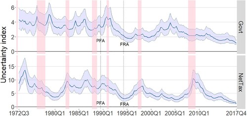
Looking at the top panel of Figure 1, we see government spending uncertainty is high (relative to the latter period) from 1972 to 1980. There are two noticeable spikes within this period: 1976 and 1978/79. Gould (1982, p. 141) notes in 1976, the newly elected National government imposed ‘sharp restraint’ to dampen down activity and reverse the expansionary influence on demand of the previous Budget. The 1978 Budget, an election year budget, saw a policy reversal with the austerity of the previous two years abandoned (Gould, 1982, p. 147). There is also a large spike in government spending uncertainty in the 1990 and 1991 years. The spike is consistent with the Treasury’s 1990 Briefing for the Incoming Minister, issued in October 1990, which warned ‘the major [economic] uncertainty centres on the fiscal outlook’ (30) as the deficits were not deemed sustainable. The government in the June 1990 Budget had relaxed fiscal policy as the election approached. After the election the new government’s response to its strained finances was to cut spending across a range of areas, with `few entitlements were left untouched, with changes affecting education, housing and employment programmes’ (Tattersfield, 2020, p. 209).

Post 1991 estimates of government spending uncertainty fall and remain relatively stable through the 1990s before increasing after the election of a new Labour government in 1999; uncertainty then peaks in 2005 before declining again. Upon Labour’s election in 1999, there was the so-called ‘winter of discontent’ – a fall in business confidence caused by concerns the government would reverse previously implemented policies. Standard and Poor’s voiced a widespread concern that ‘the economy could weaken thanks to more regulation and spending, higher taxes and a return to interventionist policies’.⁶ Ultimately, the Labour government established its fiscal credibility by scaling back its spending plans. Finally, after the Global Financial Crisis, there is a small spike in government spending uncertainty in 2011 – perhaps this reflects the government’s investments in rebuilding Christchurch after its earthquake (which would have been initially unforecastable given the variables in the model).

Looking at the lower panel of Figure 1, we see high net tax uncertainty estimates from 1972Q3 right through to the introduction of the Public Finance Act. There are three noticeable spikes in the period: 1972/73, 1982 and 1986, all of which correspond to significant tax and transfer policy changes. In the 1972 Budget, National sought to boost demand (and their election chances) through various tax cuts and increases in social welfare (see Goldsmith, 2008, p. 238 for details). The 1973 Budget saw the government introduce a 90 per cent tax rate on residential property sale profits for (non-family) houses sold within six months of purchase (Goldsmith, 2008, p. 264).

The second spike in our net tax uncertainty estimates occurs in 1982. The McCaw taskforce report, a report on the tax system, was released that year. The government followed the Taskforce’s recommendation in cutting personal taxes (Goldsmith, 2008, pp. 281–282) to make a flatter tax scale. Goldsmith (2008), however, notes the final design was complex, with rebates and surcharges used to achieve desired outcomes for different income groups. The second significant change to the tax system was the closure of tax avoidance loopholes, particularly around professionals being able to write off horticultural development expenses against their (professional) business tax liability (Goldsmith, 2008, p. 283). Goldsmith (2008, pp. 282–283) notes in closing the loophole, the government broke one of the maxims of taxation: ‘people should have certainty when confronting their tax obligations’ – the government had previously been trying to promote horticultural investment through the tax system.

Net tax uncertainty spikes again in 1986. In 1986 there were numerous tax reforms. The most significant was a collection of indirect taxes being replaced by a single consumption tax: Goods and Services Tax. After the 1986 spike, the level of net tax uncertainty generally falls until the start of 1995 with one significant blip – over 1990 and the first half of 1991. The blip corresponds with the ‘fiscal crisis’ (Dalziel & Lattimore, 2001, p. 67): the incoming government found policy in the previous Budget had not been fully costed, and revenue had been inflated via an accounting loophole. The new Minister of Finance responded by cutting welfare benefits (Dalziel & Lattimore, 2001, p. 68). The cuts were announced in December 1990 and came into effect on April 1 1991.

Between 1994 and 2017, our net tax uncertainty estimates fluctuate around a low level relative to earlier in our sample. There are notable spikes – 1996–1998, and 2008–2011 – worth comment. Between 1996–1998, the National government introduced numerous tax and transfer measures designed to incentivise beneficiaries into work. Regarding the 2008–2011 spike, there were major tax and transfer policy changes in these years. In the 2008 Budget, the government cut personal taxes. In the 2010 Budget, the corporate and top marginal personal income tax rates were cut, while the consumption (GST) tax rate was increased. Further, superannuation and all main benefits were increased.

3.1.1. Robustness of fiscal uncertainty estimates

Table 2 provides correlations between uncertainty estimates from the baseline model and the uncertainty estimates from alternative model specifications.⁷ In terms of the alternative specifications, the first is a specification where the net public debt-to-GDP ratio is added to the model and ordered last [see the correlation in row one of Table 2]. Parkyn and Vehbi (2014) incorporate a public debt constraint into their model via an identity. They note that fiscal VAR studies that ‘fail to include any feedback from the level of debt’ ‘rely on potentially mis-specified models’ (346). Dungey and Fry (2009) also include the public debt-to-GDP ratio in their study of New Zealand fiscal policy. In our sensitivity test, we follow Dungey and Fry (2009) and include the public debt-to-GDP ratio as a variable rather than via an identity.

Table 2. The Pearson correlation between uncertainty estimates from alternative specifications and the uncertainty estimate from the baseline specification for the quarters 1972Q3 to 2017Q4 (unless otherwise stated).

	Govt spending uncertainty	Net Tax uncertainty
Debt included (1982Q4 to 2017Q4)	0.75	0.96
Deterministic trend model	0.95	0.98
Model with higher output/tax elasticity	0.999	0.98
Model with 90 d rate added (1985Q2 to 2017Q4)	0.91	0.98
Time Varying Parameters model (1975Q1 to 2017Q4)	0.98	0.90

The correlation in row two of Table 2 is between the uncertainty estimates from the baseline model and the uncertainty estimates from the specification where a deterministic trend rather than stochastic trend is assumed. The correlation in row three is calculated using alternative uncertainty estimates from a specification where a higher elasticity of tax to output is assumed. Specifically, we assume 3.13 (rather than 1.2). This is the elasticity Popiel (2020) uses for his modelling in the United States, which, in turn, comes from Mertens and Ravn (2014). We feel there is value in testing a higher elasticity because Mertens and Ravn (2014), using a narrative identification approach, find the output-to-tax elasticity constructed using institutional information on the tax system is biased towards zero. Our output-to-tax elasticity (1.2), taken from Hamer-Adams and Wong (2018), is constructed using institutional information on the tax system. The correlation in row four of Table 2 is calculated using alternative uncertainty estimates from a specification where the nominal 90-day bill rate is included to control for monetary policy. The bill rate is ordered last, as per Popiel (2020). Unfortunately, we could only find quarterly 90-day bill rate data back to 1974Q1. We, therefore, only generate uncertainty estimates from 1985Q2 as we lose the first 41 observations to train the model.

Finally, we re-estimate the model with time-varying parameters (TVP) to allow for changing relationships between variables. To do this, our methodology directly follows Popiel (2020). The correlation between the uncertainty series from the TVP model and the baseline uncertainty series is reported in row five of the table. Table 2 shows, with one exception, the correlation between each alternative specification’s uncertainty estimate and the baseline specification’s uncertainty estimate is 0.9 or above.

3.2. Were the Public Finance Act and fiscal responsibility act successful in reducing uncertainty?

3.2.1. Estimates of the reduction in fiscal uncertainty

To test if net tax or government spending uncertainty fell post the introduction of the two pieces of legislation, we estimate the following regressions: (10) $\begin{array}{rl}\mathrm{Govt}.\mathrm{Uncertaint}{y}_t& ={\beta }_1+{\beta }_2\mathrm{Durin}{g}_t+{\beta }_3\mathrm{Pos}{t}_t+{\beta }_4{X}_t+{ϵ}_t\end{array}$(10) (11) $\begin{array}{rl}\mathrm{Net}.\mathrm{tax}.\mathrm{Uncertaint}{y}_t& ={\beta }_1+{\beta }_2\mathrm{Durin}{g}_t+{\beta }_3\mathrm{Pos}{t}_t+{\beta }_4{X}_t+{ϵ}_t\end{array}$(11) where Net.tax.Uncertainty_t and Govt.Uncertainty_t are the estimates of net tax and government spending uncertainty, respectively, from our baseline SVAR model. During_t  is a dummy variable that takes a value of one between 1989Q3 (the Public Finance Act came into force on 1 July 1989) and 1994Q2 (the Fiscal Responsibility Act came into force on 1 July 1994) and takes a value of zero otherwise. During_t  controls for the fact that one piece of legislation was in place in that period but not the other. Further, it also controls for the fact, as Janssen (2001, p. 29) notes: ‘the [Fiscal Responsibility] Act also codified a number of developments that had evolved in previous years’. Post_t  is a dummy variable that takes a value of one post 1994Q2 and zero otherwise – this is our variable of interest. If the two pieces of legislation have successfully reduced uncertainty, we expect the coefficient estimate on this variable to be negative and statistically significant.

Equations 10 and 11 also contain the variable X_t. This variable takes a different form in different specifications of equations 10 and 11. We omit X_t in the first specification – we call this our ‘baseline model’ (`Baseline’). In specifications (2) – (4) we control for the effects of changes in global uncertainty on uncertainty in New Zealand. A change in volatility/uncertainty overseas will spill over into New Zealand uncertainty through numerous channels, notably export demand and prices, and financial markets. In specifications (2) – (4), we use various overseas uncertainty indices to control for the impact of global uncertainty on New Zealand uncertainty. In specification (2) we use the equivalent U.S. fiscal uncertainty index from Popiel (2020) as the overseas uncertainty index (`US fiscal uncert’). So if the dependent variable in the equation is New Zealand net tax (government spending) uncertainty, we use the net tax (government spending) uncertainty variable for the United States from Popiel (2020). In specification (3) we use the output uncertainty index of Popiel (2020) (`US output uncert’) and in specification (4) we use U.S. policy uncertainty index from Baker et al. (2016) (`US BBD uncert’). The estimates of Popiel (2020) are only available until 2015Q4; hence specifications including his variables are estimated on eight fewer observations than the other specifications we estimate.

In addition to overseas uncertainty indices, we use some other variables as controls. In specification (5), we control for the lag of quarterly inflation growth (`Inflation’). The Reserve Bank of New Zealand Act 1989 (RBNZ Act) – with its purpose that the Reserve Bank will conduct monetary policy to promote stable price growth – came into effect in February 1990. It may be that a more stable inflationary environment, rather the revised fiscal legislation lowered fiscal uncertainty. Another hypothesis is that the reporting and transparency provisions of the now Public Finance Act (the original Public Finance Act 1989, with the Fiscal Responsibility Act 1994 added) did not cause a reduction in fiscal uncertainty. Rather the Act reduces fiscal uncertainty by ensuring fiscal sustainability: lower government debt lowers uncertainty about fiscal policy. In specification (6), we control for (the lag of) the government-debt-to-GDP ratio (`Debt’). If the Post variable is not statistically significant in specification (6) but is statistically significant in specification (1), it would suggest that any reduction in fiscal uncertainty is coming via the Act ensuring better outcomes for fiscal sustainability or reducing fiscal space, rather than the transparency, predictability and reporting provisions of the Act. In specification (7), we use the lag of the output gap as the variable X_t in equations 10 and 11.⁸ We see value in controlling for the output gap given, one, uncertainty increases during recessions and, two, New Zealand recessions have their genesis in overseas developments (Reddell & Sleeman, 2008). Therefore we control for the output gap to ensure that a high prevalence of recessions prior to 1989 is not driving higher uncertainty in that period (if that is what we observe).⁹ Specification (8) has dummies for any quarters where we interpolated fiscal data (1979Q2 to 1982Q1) using our Kalman smoother/Chow-Lin method (see the Online Supplementary Materials for further discussion) to make sure any peculiarities in these quarters are not driving our results. Specification (9) includes dummies for the quarter of, and the three quarters after, four major pieces of tax and transfer reform: the 1972 tax and transfer reform, the 1973 tax reform, the 1982 tax reform, and the 1986 introduction of the new consumption tax: GST. We identified in section 3.1 that spikes in net tax uncertainty were associated with tax reform events. We, therefore, run this specification to see if any heightened net tax uncertainty prior to 1989 solely reflects these tax reform events. Finally, the fiscal reforms discussed in this paper, were part of a broader set of New Zealand economic reforms in the 1984Q3 to 1995Q4 period, which saw domestic markets, trade, and financial markets liberalised (Evans et al., 1996). Our final specification (10) has dummies for the whole economic reform period: 1984Q3 to 1995Q4. We motivate this specification by arguing that the broader reform in New Zealand in the 1984Q3 to 1995Q4 period might have heightened uncertainty, and this uncertainty might have dissipated once the institutional reform was complete, regardless of whether the fiscal policy legislation was changed.

Table 3 reports the results from estimating equations 10 and 11 with no additional covariates (i.e. specification 1). We estimate (by looking at the coefficient estimate on the Post variable) that in the period post the introduction of both pieces of legislation, net tax uncertainty fell 39 per cent (−2.913/7.379) relative to the quarters in our sample prior to the legislation’s introduction. The percentage reduction is calculated by dividing the coefficient estimate on the Post variable by the Constant/intercept estimate (as the constant represents, for our sample, the estimate of the mean of net tax uncertainty before the Public Finance Act was enacted in 1989). We estimate government spending uncertainty fell 38 percent (−1.423/3.659) post the introduction of both pieces of legislation. The coefficient estimates on the Post variable reported in Table 3 are both significant at a one per cent level. We use HAC standard errors to assess statistical significance.¹⁰

Table 3. The estimated effect of the fiscal policy legislation on fiscal uncertainty: baseline model results.

	Net tax	Government spending
	(1)	(2)
During	−1.075	−0.302
	(0.889)	(0.337)
Post	−2.913***	−1.423***
	(0.641)	(0.152)
Constant	7.379***	3.659***
	(0.506)	(0.102)
Observations	182	182
R^2	0.31	0.59
F statistic (df = 2, 179)	40.4	128.4

Note: HAC standard errors reported.

Figure 2 presents our estimates of the percentage reduction in fiscal uncertainty from the alternative specifications described in the previous text. The underlying regression results are available in the Online Supplementary Materials (see Tables 1–4; the estimate on the Post variable is statistically significant at a one percent level in all the alternative specifications). Figure 2 also presents estimates of the percentage reduction in uncertainty from estimating equations 10 and 11 (with no additional covariates) but with fiscal uncertainty from the time-varying parameters SVAR model as the dependent variable (‘TVP’). Finally, Figure 2 also presents our estimates of percentage reduction in uncertainty from various subsamples. For the subsample models, we reestimate the SVAR on the subsample and use the uncertainty estimates from the subsample SVAR as the dependent variables in estimating equations 10 and 11 (with no additional covariates). Again, the estimate on the Post variable is statistically significant at a one percent level in all subsamples (see Tables 5 and 6 in the Online Supplementary Materials for the complete regression tables for the subsamples).

Figure 2. Estimates of the percent reduction in mean uncertainty: alternative specifications and subsamples.

Note: The regression results underpinning this figure are available in Tables 1–6 of the Online Supplementary Materials. ‘Baseline’ is specification (1): the baseline model with no additional covariates; ‘US fiscal uncert’ is the baseline model with either US government or net tax uncertainty added as a covariate (see text for discussion); ‘US output uncert’ is the baseline model with US output uncertainty added as a covariate; ‘US BBD uncert’ is the baseline model with the US economic policy uncertainty of Baker et al. (2016) added as a covariate; ‘Inflation’, ‘Debt’ and ‘Output gap’ are specifications consisting of the baseline model with inflation, the government net debt-to-GDP ratio, and the output gap added as covariates respectively; ‘TVP’ is the time-varying parameters version of the baseline model; ‘Interpolated = 1’, ‘Major reform = 1’ and ‘All reform = 1’ is the baseline model with dummies for interpolated quarters, major tax reform quarters and the economic reform quarters respectively (see the text for more information); ‘1983-2017’, ‘1983-2010’ and ‘1972-2010’ are the results from the baseline model estimated on those subsamples.

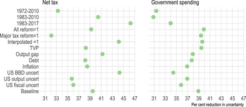
Table 1. P-values for a test of the null hypothesis of stationarity using the KPSS approach.

	log(Net tax)	log(Government spending)	log(GDP)
Trend, intercept	0.01	0.01	0.01
Intercept	0.01	0.01	0.01

Note: All three variables are real and expressed in per capital terms.

Figure 2 (left panel) shows that either adding dummy variables for our interpolated quarters or excluding the quarters between 1972Q3 and 1983Q2 from our sample result in higher estimates of the reduction in net tax uncertainty owing to the legislation than in our baseline model over the full sample. On the other hand, excluding the years 2010–2017 lowers our estimates of the uncertainty reduction. Adding the U.S. net tax and output uncertainty indices of Popiel (2020) results in lower estimates of the reduction in net tax uncertainty than in our baseline model, as does adding dummy variables for quarters with major tax reform. Collectively, the estimates of the reduction in net tax uncertainty owing to the legislation from our alternative specifications suggest that the balance of risks around our estimate from our baseline model (a 39 per cent reduction) are fairly even. Our results suggest a plausible range for the estimates of reduction in net tax uncertainty owing to the now Public Finance Act of between 32 and 46 per cent.

In contrast, the right panel of Figure 2 suggests our estimate of a 38 per cent reduction in government spending uncertainty owing to the legislation from our baseline model might be at the top end of plausible estimates. Removing the quarters between 2011Q1 to 2017Q4, in particular, reduces the estimates of the fall in government spending uncertainty post the legislation’s introduction by around eight percentage points. In discussing the data construction in the Online Supplementary Materials, we note 1972Q1 had an unusual value for government spending. If this value is removed from our data set, the estimated reduction in government spending uncertainty is 34 per cent (see the row `1983-2017’ in the right-hand panel of Figure 2). The additional covariates our estimates of the reduction in government spending uncertainty are most sensitive to are: the U.S. government spending and output uncertainty variables of Popiel (2020) and the U.S. policy uncertainty index of Baker et al. (2016). Our results suggest a plausible range for the estimates of reduction in government spending uncertainty owing to the now Public Finance Act of between 31 and 40 per cent.

There are results from one specification we want to discuss in more detail: specification (6), where we control for the government-debt-to-GDP ratio. As noted above if the results were materially different between baseline specification and specification (6), it would suggest that any reduction in fiscal uncertainty is coming via the Act ensuring better outcomes for fiscal sustainability and/or restricting fiscal space, rather than the transparency, predictability and reporting provisions of the now Public Finance Act. Regarding the connection between fiscal space and fiscal uncertainty, there is an analogy to inflation. It is well known that when inflation is high, inflation outcomes are more variable and thus inflation targeting indirectly reduces the variability in inflation even though it is focused on the level of inflation. If fiscal variables are more variable when they are subject to less restrictions, we could have expected the Public Finance Act to indirectly reduce the variability in fiscal variables by restricting the growth in debt (and thus restricting the choices available to politicians around government spending, taxes and transfers). For both government spending and net tax uncertainty, the estimates in the reduction in uncertainty owing to the Public Finance Act are similar between the specifications with and without government debt (see Figure 2 and compare the `Baseline’ and `Debt’ estimates), suggesting the fiscal sustainability/fiscal space channel is not a strong channel through which fiscal uncertainty is reduced.

3.3. The impact of fiscal policy uncertainty on output

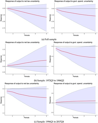
In this section, we answer our second research question: what is the impact of fiscal uncertainty on output? Our results from the baseline SVAR model estimated on the full sample suggest that fiscal uncertainty is not detrimental to output. Figure 3(a) plots the relevant impulse responses; the impulse responses are the output responses to a one log-point uncertainty shock, i.e. a doubling of uncertainty. We see that, over our full sample, neither net tax nor government spending uncertainty affects output growth.

Figure 3. Response of output to a surprise doubling in fiscal uncertainty: baseline SVAR model.

Note: The shaded area represents the 68 percent credible set. The red line is posterior median. The y-axis is in percent growth rates.

As discussed earlier, over the course of our sample period there was a significant shift in the role of government played in the New Zealand economy. Prior to early 1984, both Wells (1987) and Buckle (2018) note that the government utilised fiscal policy as a means of actively managing demand. White (2013, ii) argues that in the period: `monetary policy was constrained by impediments to interest rate flexibility; fiscal policy became, if anything, more activist, and increasingly a prop for the economy’. One component of this activist fiscal policy was an episode of state-led industrialisation beginning in the late-1970s and peaking in 1983/84, known as the ‘Think Big’ projects. The projects were mainly state guaranteed (Wells, 1987, p. 291) and as such would not be counted as government investment (and therefore would not count as government spending in our modelling framework). As part of Think Big, however, there were still significant state-funded projects that would count as government investment. Boshier (1984, p. 59) notes the contribution of publicly-financed energy investment kept government investment at a reasonably high level during the period. Further, as Easton (2020, p. 464) notes there was significant government investment, such as roads and harbours, to support the `Think Big’ projects.

In addition to its use of activist fiscal policy, another way the government was a significant player in the pre-reform period was its role as producer of market goods either through government trading departments or state-owned enterprises (see Evans et al., 1996, p. 1860). Government production was supported by significant government investment. The government played the primary role in building electricity generating schemes and building and maintaining the electricity transmission network prior to the mid-1980s. Further the government, via the Housing Corporation, was tackling the housing shortage by building state houses in the mid-1970s (see Bassett, 2013, p. 331). These are only two of many examples.

The active role the government played in the economy meant any uncertainty about government decisions was a substantial source of uncertainty for firms. Government spending uncertainty meant demand uncertainty for firms from whom the government directly or indirectly purchased. Further, as a provider of many key services for firms – transport, electricity and the telecommunications, to name a few – any uncertainty about government investment in these services affected the investment decisions of firms whose investment plans were contingent on these services. Finally, with monetary policy constrained, any uncertainty about fiscal policy could not be offset by looser monetary policy.

Once the reforms were completed, however (and in many cases before), there were several significant changes to the role of government. Many government entities were privatised (see Evans et al., 1996) reducing government investment, state-led industrialisation ceased, and fiscal policy took a more medium-run focus (see Barker, Buckle, St, & Clair, 2008). Monetary policy was entrusted with stabilisation and was therefore free to offset any effects of government spending uncertainty. Collectively, this suggests that output’s response to government spending uncertainty might be time dependent. Specifically, given the significant government role in the economy in the pre-reform period, and the inability of monetary policy to offset government spending uncertainty, we would expect that government spending uncertainty would be more detrimental to output in the pre-reform period than in the post reform period. To test this, we split the data into a pre-reform sample – 1972Q3-1984Q2 – and a post-reform sample – 1996Q1-2017Q4.¹¹ We choose 1996Q1 to be the start of post-reform sample, as the bulk of the reforms where complete by 1995 (see Evans et al., 1996, Figure 2).

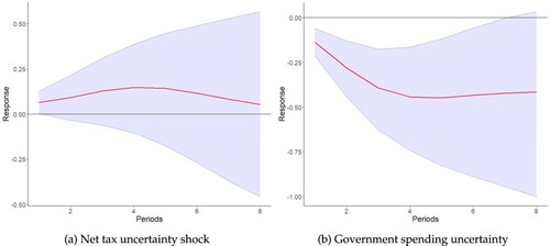
The second and third rows of Figure 3(b) plot the impulse responses for the pre – and post-reform periods. We see that a doubling of government spending uncertainty lowers output in the pre-reform period (by 0.5 per cent after six quarters) but has no effect in the post-reform period. This result is consistent with the hypotheses we set out above. In the pre-reform period government was a more important player in the economy and thus uncertainty about government demand would have been more detrimental to firm investment and therefore GDP. Secondly, with monetary policy restricted (for reasons discussed above) in the pre-reform period, monetary policy was not able to offset any falls in GDP owing to reduced firm investment as the result of government spending uncertainty.¹² In the post-reform period, the finding that government spending uncertainty has no impact on output is consistent with: (1) government’s lesser role in the economy and (2) monetary policy being able to act to offset the negative effects of reduced investment spending owing to government spending uncertainty. As evidence for this second channel, panel (b) of Figure 4 shows that in the version of the model that includes the short-term (nominal 90-day) interest rate, monetary policy did appear to offset government spending uncertainty over the period 1985Q2 to 2017Q4 (the bulk of which is the post-reform period).¹³

Figure 4. Response of the nominal 90 d bank bill rate to a surprise doubling in fiscal uncertainty in SVAR model with the short-term interest rate added: 1985Q2 to 2017Q4. (a) Net tax uncertainty shock. (b) Government spending uncertainty shock.

Note: The shaded area represents the 68 percent credible set. The red line is posterior median. The y-axis is in percentage points.

On the other hand, a doubling of net tax uncertainty has no statistically significant effect on output in the pre-reform period but has a (small) negative effect on output on impact in the post-reform sample. Specifically, we find that doubling net tax uncertainty lowers output by 0.1 per cent on impact in the post-reform sample. This finding that net tax uncertainty has a negative effect on output is consistent with the studies of Fernández-Villaverde et al. (2015), Mumtaz and Surico (2018) and the baseline model of Popiel (2020).¹⁴ To explain why the impact of net tax uncertainty on output changes between the pre – and post-reform periods, we note that before 1984 potentially two competing mechanisms were at play regarding tax uncertainty. The first mechanism is firms, when tax policy is uncertainty high, hold off investment and hiring until tax policy becomes clearer (Pindyck, 1990); this will lower output. A similar argument can be made about households and durable consumption. This ‘wait and see’ argument suggests net tax uncertainty should lower output. The second mechanism, which meant net tax uncertainty might increase output, reflects the distinctive role the tax system played before the reform (Goldsmith, 2008, p. 283). The tax system promoted (export) development through concessions and incentives – Bassett (2013, p. 343) provides numerous examples, including concessions and incentives for forestry, fishing and horticulture. Hassett and Metcalf (1999) argue that investment tax credits follow a random walk process because (1) investment tax credits tend to stay at the same value for few years, and (2) they are also mean reverting. Hassett and Metcalf (1999) show in such circumstances tax credit uncertainty boosts investment: ‘[b]ecause the firm fears that the credit might be eliminated, it is more likely to invest today while the credit is still effective ‘(Hassett & Hubbard, 1996), p. 40). Certainly, in New Zealand prior to 1984 it was likely tax concessions and incentives could be reversed. Indeed, in section 3.1 we gave the example where tax concessions for horticultural development were discontinued unexpectedly. More generally, the government was often forced into rapid changes in fiscal policy in the 1970s if foreign exchange reserves were short. Prior to 1984, the net result of the two opposing mechanisms articulated above operating was they cancelled each other out and net tax uncertainty had no statistically significant impact on output. Post-1995, the first mechanism – firms (and households) waiting and seeing under uncertainty and thereby lowering investment, new hires and (durable) consumption – is likely to be still operating, as although tax policy plays less of a stabilisation role, it still affects key relative prices in the economy. However, as the tax system is no longer used (as much) to promote industries via concessions and incentives, the second mechanism discussed above operates less.

We end this section by discussing one limitation and one puzzle regarding the analysis in this section. The limitation is that, by reporting the impulse responses from the SVAR model without time varying parameters, we are assuming the relationships between the variables in model are constant through time. If this assumption is not true, this has implications for reliability of impulse responses via two sources: (1) fiscal uncertainty (and the fiscal uncertainty shocks) might be mismeasured and (2) the estimated responses to the uncertainty shock might be incorrect. The puzzle is why monetary policy responds to government spending uncertainty but net tax uncertainty does not (see Figure 4); we leave resolving this puzzle to further research.

4. Conclusion

This paper analyses if the now Public Finance Act (1989) (which incorporates the Fiscal Responsibility Act, 1994) lowered uncertainty about fiscal policy. We use data assembled from various sources covering the period from 1961Q2 to 2017Q4. And by adding a stochastic volatility term to the standard model for estimating fiscal multipliers (following the methodology of Popiel, 2020), we estimate government spending and net tax uncertainty for the 1972Q3 to 2017Q4 quarters. Our results suggest that after the introduction of the Fiscal Responsibility Act in 1994, net tax uncertainty was between 32–46 per cent lower, on average, than its level in the quarters in our sample that precede the Public Finance Act (1989). After the introduction of the Fiscal Responsibility Act in 1994, government spending uncertainty was between 31–40 per cent lower, on average, than its level before the Public Finance Act was enacted in 1989. Based on this evidence, we conclude the Public Finance Act (1989) and Fiscal Responsibility Act (1994) successfully reduced fiscal policy uncertainty.

This paper also presents estimates of the impact of fiscal uncertainty on output. Under the current tax structure, where tax is used less to promote investment through concessions and incentives, we find net tax uncertainty adversely affects output. Specifically, we find that doubling net tax uncertainty lowers output by 0.1 per cent on impact, which is not a large effect. In the period 1972Q3 to 1984Q2 when government spending was more activist, we found that a doubling in government spending uncertainty lowered output by 0.5 per cent. However, in more recent times, we find that government spending uncertainty has no statistically significant effect on output. In terms of why this has occurred, monetary policy, under current institutional arrangements, acts to offset the negative effects of government spending uncertainty. Further, the government is less of source of demand than it was prior to the New Zealand economy’s reform.

We undertake numerous robustness checks and show that the key result – the legislation was associated with lower fiscal uncertainty – still holds. Our set of checks are centred around establishing the sensitivity of our fiscal uncertainty estimates to alternative specifications of our SVAR. To test the sensitivity of our fiscal uncertainty estimates from our SVAR model, we add monetary policy and public debt as additional variables to the model. We also relax key assumptions about imposed elasticities and the appropriate trend; we also run a specification where the parameters of the model are allowed to change through time. We find little change in our estimated fiscal uncertainty series. The correlation with the relevant fiscal uncertainty series from the alternative specifications and the baseline model is 0.9 or above (with one exception). We also check the robustness of our regression estimates of the reduction in fiscal uncertainty after the introduction of the now Public Finance Act. To do this, we estimate the regression on different subsamples and control for various potential explanatory variables. Our estimates of the effect of the legislation’s introduction on uncertainty remain broadly similar and statistically significant.

Two pieces of further research immediately comes to mind. Our measure of uncertainty is based on the dispersion in one-step-ahead forecast errors. It would be worth using alternative measures of fiscal policy uncertainty – particularly, the newspaper-based measures of Baker et al. (2016) – to see if the results change. This is not possible at present as more of New Zealand’s historical newspapers prior to the 1990s need to be digitised to construct newspaper-based measures. Newspaper-based measures would pick up uncertainty about fiscal proposals that never see the light of day, such as the recent debate in New Zealand about the capital gains tax. Our measure will miss the uncertainty from such proposals. Secondly, at present, the model assumes that there is no spillover of tax uncertainty to government spending uncertainty (and vice versa). This is an assumption that might not always hold true and could be relaxed in further work.

Acknowledgements

We would like to thank the referees, Bob Buckle, Kam Szeto, John Janssen, John McDermott Les Oxley and participants at the 2022 New Zealand Association of Economists’ conference for comments on an earlier draft. Thanks to Carol Mitchell of Statistics New Zealand for answering questions on SNA definitions and to Michal Popiel for sharing his code. All errors are our own. This research was undertaken while the first author was on a University of Waikato PhD scholarship.

Disclosure statement

No potential conflict of interest was reported by the author(s).

Notes

1 The quotes are from Buckle (2018), The Economist (1995) and Ball (2019) respectively.

2 For example, the legislation requires the government to follow the principles of: (1) managing ‘prudently the fiscal risks facing the government’, and (2) when formulating revenue strategy, having regard to ‘predictability and stability of tax rates’.

3 Cross country evidence that fiscal policy volatility is detrimental to output/economic growth is also presented by Afonso and Furceri (2010), Ramey and Ramey (1995), Fatás and Mihov (2003) and Fatás and Mihov (2013).

4 Ali, Badshah, Demirer, and Hegde (2022) create a similar index for New Zealand and find uncertainty spikes in similar places.

5 Allowing for two lags of fiscal uncertainty to affect the other variables in the model is a departure from Popiel (2020) who only allows fiscal uncertainty to have a contemporaneous impact only. We argue this is appropriate as there is often a lag from the investment decision (which is affected by fiscal uncertainty) and implementation and therefore being counted in GDP.

6 The Online Supplementary Materials contains the estimated parameters of the stochastic volatility equations.

7 The quote is from The Spinoff, June 7 2018, Does Jacinda Ardern face a Helen Clark style winter of discontent? available at: https://thespinoff.co.nz/politics/07-06-2018/does-jacinda-ardern-face-a-helen-clark-style-winter-of-discontent [accessed 8 February 2022].

8 The plots of the alternative uncertainty series are available in Figure 6 of the Online Supplementary Materials.

9 This is created by applying the filter of Kamber, Morley, and Wong (2018) to our GDP series.

10 The coefficient on the output gap should be treated with caution. There is potential endogeneity between uncertainty and the output gap.

11 Our Online Supplementary Materials reports a test for unknown structural breaks in both uncertainty time series. For both fiscal uncertainty series we find the break at 1992Q4. This suggests that earlier falls in uncertainty (i.e. pre the two Acts being enacted) did not result in our ‘Post’ variable being statistically significant.

12 These are the quarters the model produces uncertainty estimates for. The estimation period begins five years earlier as the 40 quarters prior to the start of the estimation period are used as model training quarters (plus one quarter is lost owing to the stochastic trend assumption).

13 Numerous studies have concluded that uncertainty shocks are demand shocks and therefore the central bank will cut its policy rate in response; see Kamber, Karagedikli, Ryan, and Vehbi (2016) for New Zealand evidence.

14 As a reminder, the estimation period of the version of the model that includes the short-term interest rate is restricted by availability of the interest rate series (see section 3.1).

15 Unlike Popiel (2020) when we add monetary policy to the model estimated on the 1996–2017 sample, net tax uncertainty still has a statistically significant effect on output; see Figure 7 in the Online Supplementary Materials.

References

- Afonso, A., & Furceri, D. (2010). Government size, composition, volatility and economic growth. European Journal of Political Economy, 26(4), 517-532. doi:10.1016/j.ejpoleco.2010.02.002
- Albuquerque, B. (2011). Fiscal institutions and public spending volatility in Europe. Economic Modelling, 28(6), 2544–2559. doi:10.1016/j.econmod.2011.07.018
- Ali, S., Badshah, I., Demirer, R., & Hegde, P. (2022). Economic policy uncertainty and institutional investment returns: The case of New Zealand. Pacific-Basin Finance Journal, 74, 101797. doi:10.1016/j.pacfin.2022.101797
- Anzuini, A., & Rossi, L. (2021). Fiscal policy in the US: A new measure of uncertainty and its effects on the American economy. Empirical Economics, 61, 2613–2634. doi:10.1007/s00181-020-01984-3
- Anzuini, A., Rossi, L., & Tommasino, P. (2020). Fiscal policy uncertainty and the business cycle: Time series evidence from Italy. Journal of Macroeconomics, 65, 103238. doi:10.1016/j.jmacro.2020.103238
- Badinger, H., & Reuter, W. H. (2017). The case for fiscal rules. Economic Modelling, 60, 334–343. doi:10.1016/j.econmod.2016.09.028
- Baker, S., Bloom, N., & Davis, S. (2016). Measuring economic policy uncertainty. Quarterly Journal of Economics, 131(4), 1593–1636. doi:10.1093/qje/qjw024
- Ball, I. (2019). Public Finance Act has proved its worth in good times and bad. Stuff NZ. Retrieved February 18, 2022, from https://www.stuff.co.nz/national/politics/opinion/114464570/ public-finance-act-has-proved-its-worth-in-good-times-and-bad.
- Barker, F., Buckle, C., St, R., & Clair, R. (2008). Roles of fiscal policy in New Zealand (Working paper No. 2/2008). New Zealand Treasury. https://www.treasury.govt.nz/publications/wp/ roles-fiscal-policy-new-zealand-wp-08-02-html.
- Bassett, M. (2013). The state in New Zealand, 1840-1984: Socialism without doctrines? Auckland: Auckland University Press.
- Beckmann, J., & Czudaj, R. L. (2021). Fiscal policy uncertainty and its effects on the real economy: German evidence. Oxford Economic Papers, 73(4), 1516–1535. doi:10.1093/oep/gpab009
- Blake, A. P., Mumtaz, H., et al. (2012). Applied Bayesian econometrics for central bankers. Centre for Central Banking Studies, Bank of England. https://www.bankofengland.co.uk/ccbs/applied-bayesian-econometrics-for-central-bankers-updated-2017.
- Blanchard, O., & Perotti, R. (2002). An empirical characterization of the dynamic effects of changes in government spending and taxes on output. Quarterly Journal of Economics, 117(4), 1329–1368. doi:10.1162/003355302320935043
- Boshier, J. F. (1984). Energy issues and policies in New Zealand. Annual Review of Energy, 9(1), 51–79. doi:10.1146/annurev.eg.09.110184.000411
- Buckle, R. (2018). A quarter of a century of fiscal responsibility: The origins and evolution of fiscal policy governance and institutional arrangements in New Zealand, 1994 to 2018 (Chair in Public Finance Working paper No. 13/2018). Victoria University of Wellington. https://ir.wgtn.ac.nz/handle/123456789/20848.
- Claus, I., Gill, A., Lee, B., & McLellan, N. (2006). An empirical investigation of fiscal policy in New Zealand (Working paper No. 6/2008). New Zealand Treasury. https://www.treasury.govt.nz/sites/default/files/2007-09/twp06-08.pdf.
- Dalziel, P., & Lattimore, R. (2001). The New Zealand macroeconomy: A briefing on the reforms and their legacy. Melbourne: Oxford University Pres.
- De Haan, J., Jong-A-Pin, R., & Mierau, J. O. (2013). Do budgetary institutions mitigate the common pool problem? New empirical evidence for the EU. Public Choice, 156(3), 423–441. doi:10.1007/s11127-012-9949-5
- Dungey, M., & Fry, R. (2009). The identification of fiscal and monetary policy in a structural VAR. Economic Modelling, 26(6), 1147–1160. doi:10.1016/j.econmod.2009.05.001
- Easton, B. (2020). Not in narrow seas: The economic history of Aotearoa New Zealand. Wellington: Victoria University Press.
- Evans, L., Grimes, A., Wilkinson, B., & Teece, D. (1996). Economic reform in New Zealand 1984-95: The pursuit of efficiency. Journal of Economic Literature, 34(4), 1856–1902. https://EconPapers.repec.org/RePEc:aea:jeclit:v:34:y:1996:i:4:p:1856-1902.
- Fatás, A., & Mihov, I. (2003). The case for restricting fiscal policy discretion. The Quarterly Journal of Economics, 118(4), 1419–1447. doi:10.1162/003355303322552838
- Fatás, A., & Mihov, I. (2006). The macroeconomic effects of fiscal rules in the US states. Journal of Public Economics, 90(1-2), 101–117. doi:10.1016/j.jpubeco.2005.02.005
- Fatás, A., & Mihov, I. (2013). Policy volatility, institutions, and economic growth. Review of Economics and Statistics, 95(2), 362–376. doi:10.1162/REST_a_00265
- Fernández-Villaverde, J., Guerrón-Quintana, P., Kuester, K., & Rubio-Ramırez, J. (2015). Fiscal volatility shocks and economic activity. American Economic Review, 105(11), 3352–3384. doi:10.1257/aer.20121236
- Gill, D. (2019). The Fiscal Responsibility Act 1994: How a nonbinding policy instrument proved highly powerful. In Successful public policy: Lessons from Australia and New Zealand (pp. 423–452). Canberra: ANU Press.
- Goldsmith, P. (2008). We won, you lost, eat that!: A political history of tax in New Zealand since 1840. Auckland: David Ling Publishing.
- Gould, J. D. (1982). The rake’s progress?: The New Zealand economy since 1945. Auckland: Hodder. Stoughton.
- Hall, V., & McDermott, C. J. (2016). Recessions and recoveries in New Zealand’s post-Second World War business cycles. New Zealand Economic Papers, 50(3), 261–280. doi:10.1080/00779954.2015.1129358
- Hamer-Adams, A., & Wong, M. (2018). Quantifying fiscal multipliers in New Zealand: The evidence from SVAR models (Analytical note No. 2018/05). Reserve Bank of New Zealand. https://www.rbnz.govt.nz/hub/publications/analytical-note/2018/an2018-05.
- Hassett, K. A., & Hubbard, R. G. (1996) Tax policy and investment (Working Paper, w5683). NBER.
- Hassett, K. A., & Metcalf, G. E. (1999). Investment with uncertain tax policy: Does random tax policy discourage investment. The Economic Journal, 109(457), 372–393. doi:10.1111/1468-0297.00453
- Janssen, J. (2001). New Zealand’s fiscal policy framework: Experience and evolution (Working paper No. 01/25). New Zealand Treasury. https://www.treasury.govt.nz/publications/wp/new-zealands-fiscal-policy-framework-experience-and-evolution-wp-01-25.
- Kamber, G., Karagedikli, O., Ryan, M., & Vehbi, T. (2016). International spill-overs of uncertainty shocks: Evidence from a FAVAR (Working paper No. 61/2016). Centre for Applied Macroeconomic Analysis, Crawford School of Public Policy. https://papers.ssrn.com/sol3/papers.cfm?abstract_id=2848034
- Kamber, G., Morley, J., & Wong, B. (2018). Intuitive and reliable estimates of the output gap from a Beveridge-Nelson filter. The Review of Economics and Statistics, 100(3), 550–566. doi:10.1162/rest_a_00691
- Kwiatkowski, D., Phillips, P., Schmidt, P., & Shin, Y. (1992). Testing the null hypothesis of stationarity against the alternative of a unit root: How sure are we that economic time series have a unit root? Journal of Econometrics, 54(1), 159–178. doi:10.1016/03044076(92)90104-y
- Lees, K. (2020). Introducing the New Zealand Economic Uncertainty Index (Technical report). Sense Partners. https://static1.squarespace.com/static/575e7fd9b09f95d77dded61a/t/%20%5Cnewline%205f3dbb9fbd8be23608d8daf7/1597881250530/Quantifying+the+impacts+of+economic+uncertainty+introducing+the+New+Zealand+Economic+Uncertainty+Index+FINAL.pdf.
- Mertens, K., & Ravn, M. (2014). A reconciliation of SVAR and narrative estimates of tax multipliers. Journal of Monetary Economics, 68, S1–S19. doi:10.1016/j.jmoneco.2013.04.004
- Mumtaz, H., & Surico, P. (2018). Policy uncertainty and aggregate fluctuations. Journal of Applied Econometrics, 33(3), 319–331. doi:10.1002/jae.2613
- Parkyn, O., & Vehbi, T. (2014). The effects of fiscal policy in New Zealand: Evidence from a VAR model with debt constraints. Economic Record, 90(290), 345–364. doi:10.1111/1475-4932.12116
- Pindyck, R. (1990). Irreversibility, uncertainty, and investment. Journal of Economic Literature, 29(3), 1110.
- Popiel, M. (2020). Fiscal policy uncertainty and US output. Studies in Nonlinear Dynamics & Econometrics, 24(2), 1–27. doi:10.1515/snde-2018-0024
- Ramey, G., & Ramey, V. A. (1995). Cross-country evidence on the link between volatility and growth. American Economic Review, 85(5), 1138–1151. http://www.jstor.org/stable/2950979.
- Reddell, M., & Sleeman, C. (2008). Some perspectives on past recessions. Reserve Bank of New Zealand Bulletin, 71(2), 5–21. https://www.rbnz.govt.nz/%7Bresearch-and-publications/reservebank-bulletin/2008/rbb2008-71-02-01%7D.
- Tattersfield, B. (2020). Bill Birch: Minister of everything. Auckland: Mary Egan Publishing.
- Wells, G. (1987). The changing focus of fiscal policy. In Allan Bollard & Robert Buckle (Eds.), Economic liberalisation in New Zealand (pp. 283–298). Allen & Unwin.
- White, B. (2013). Macroeconomic policy in New Zealand: From the great inflation to the global financial crisis (Working paper No. 13/30). New Zealand Treasury. https://ideas.repec.org/p/nzt/nztwps/13-30.html.
- Woo, J. (2009). Why do more polarized countries run more procyclical fiscal policy? The Review of Economics and Statistics, 91(4), 850–870. doi:10.1162/rest.91.4.850