Carbon concentration of living tree biomass of Pinus sylvestris, Picea abies, Betula pendula and Betula pubescens in Sweden

ABSTRACT

This study examined the carbon (C) concentration of the major tree species (Scots pine, Norway spruce, and Birch) in Sweden based on destructively sampled biomass data. The examination was made using single trees and comprised three components: branches with needles, stemwood with bark, and stump with roots. We developed a weighted C concentration estimator accounting for fresh weights of tree components to infer the C concentration at the population level. Significant differences in C concentration (%) were found among species, with the highest in pine (50.671 ± 0.211), followed by spruce (49.518 ± 0.164) and the lowest in birch (49.347 ± 0.241). Additionally, the C concentration varied among tree components, regardless of tree size, growth rate, and site conditions. At the national level, we applied the estimated species- and component-specific C concentration constants to the measured total biomass of the major tree species from the National Forest Inventory. This extrapolation revealed that the average C concentration of major trees across all forestlands in Sweden was approximately 50.012%. These findings have significant implications for accurate C sequestration reporting in the LULUCF sector.

KEYWORDS:

• Boreal forests
• national forest inventory
• carbon accounting
• LULUCF
• Sweden

Introduction

Accurate estimates of the carbon (C) concentration of live trees are important when quantifying the amount of C sequestered in forests. Signatory countries to the United Nations Framework Convention on Climate Change (UNFCCC) are expected to report (in the sector of Land Use, Land Use Change and Forestry, i.e. LULUCF) changes in the living biomass C pool at the national scale. Most often, the C concentration of trees is assumed to be about 47–50% of the dry-weight biomass (IPCC 2006; Ladanai et al. 2010; Strömgren et al. 2013). However, recent studies have shown that this assumption is not entirely accurate, leading to under- or overestimation of forest C stocks (Thomas and Martin 2012). Such inaccuracies may further obscure optimal decision-making in nationwide or biome-level C accounting schemes (Thomas and Martin 2012; Ma et al. 2018). Nevertheless, the accuracy of C concentration in tree species has been improving for tropical and temperate forests during the last decade (Thomas and Martin 2012). This is a sharp contrast to the boreal forests where few studies have examined the variation in tree species’ C concentration (Gao et al. 2016).

The deviations of C concentration from the nominal value of 50% are most often ascribed to differences in site conditions (Ma et al. 2018), tree species (Thomas and Martin 2012), and tree components (Gao et al. 2016). In a global meta-analysis study, Ma et al. (2018) reported a decrease in plant C concentration with increasing latitude. From a comprehensive review of 31 studies, Thomas and Martin (2012) found that tree C concentration varied widely across tree species ranging from 41.9–51.6% in tropical species, 45.7–60.7% in subtropical/Mediterranean species, and 43.4–55.6% in both temperate and boreal species. The distribution of C concentration is significantly different among tree components – i.e. the leaves, branches, bark, stems, and roots. Conifers, relative to broadleaved trees, have higher C concentrations in roots, leaves, and stems (Ma et al. 2018). In addition, based on 165 sample trees, Gao et al. (2016) found larger C concentration in the bark (56.2%) than in the stemwood (50.5%) of major tree species (such as jack pine, trembling aspen, white birch, black and white spruce, and balsam fir) of the boreal forests in North America. Similar findings have also been reported for temperate tree species (Bert and Danjon 2006; Martin et al. 2015). In an experiment with 27-year-old stands on set-aside farmlands, Alriksson and Eriksson (1998) reported no significant species-related C distribution in vegetation compartments of five tree species (including Pinus sylvestris L., Picea abies L. Karst., and Betula pendula Roth) in northeastern Sweden.

Other factors such as tree size and social position (i.e. dominant and suppressed) have also been suggested to affect the C concentration of living trees. By comparing 16 Neotropical trees, saplings had a higher C concentration than large trees (Martin et al. 2013). In two Caribbean rainforest trees, the C concentration in wood increased linearly with the diameter at breast height (Martin and Thomas 2013). Gao et al. (2016) reported increased C concentration in stemwood and bark with tree size for shade-intolerant species, whereas those of shade-tolerant species exhibited negative or neutral size-carbon associations in the boreal forest of North America.

The discrepancies are difficult to explain and suggest that detailed information on tree species and component-specific C concentration is needed for the accurate reporting of C sequestration in the LULUCF sector. The extent to which C concentration varies among tree species and within tree components, along a climatic gradient from north to south Sweden remains to be assessed. To the best of our knowledge, no study has weighed the C concentration at the national scale by integrating the information on weighted tree-level carbon and total biomass. This study aimed to examine the C concentration in the major tree species in Swedish forests along a latitudinal gradient. The tree species examined were Scots pine (Pinus sylvestris L.), Norway spruce (Picea abies L. Karst.) and birch (Betula pendula and Betula pubescens), which together contribute to more than 90% of the total volume of the growing stock on forestlands. Specifically, we sought to (1) examine the differences in C concentration between species, (2) the differences in C concentration between tree components for a given species, (3) evaluate the variation in C concentration along the stem, and (4) investigate the influence of tree (e.g. species, diameter, age, health), stand and site characteristics (e.g. site index, basal area, height, soil type) on the C concentration in tree components. We analysed empirical data obtained from destructive biomass sampling of sample trees in stands distributed across latitudes 57–64 °N. The data analysed in the present study was part of the material used by Petersson and Ståhl (2006) to develop below-ground biomass functions for the major tree species in Sweden. For inference, we developed a weighted C concentration estimator that takes into consideration the variations among trees. For upscaling to the national level, we applied the weighted C concentration constants for each tree species and component to the latest inventory data of the Swedish National Forest Inventory.

Materials and methods

Study sites and stand selection

The laborious and expensive nature of biomass measurements demands efficient sampling methods. Practical considerations and the demand for efficiency led to a stepwise procedure where stands, plots, trees and dry-weight samples were selected and measured. In the summer of 2002, six stands from the north (Svartberget, 64° N, 19° E), three stands from the middle (Jädraås, 60° N, 16° E), and three stands from the southern part of Sweden (Asa, 57° N, 14° E) were subjectively selected (Petersson and Ståhl 2006). The stands were selected in such a way that they covered the latitudinal growth conditions in Sweden (Figure 1). The stand selection was made with the following restrictions; (1) that spruce, pine and birch should together account for at least 50% of the basal area and (2) that the stand mean height should exceed 1.3 m. Within these stands, up to three sample plots with a radius of 10 m were laid out at random (26 plots in total). Standard stand and site characteristics were measured on the plots. About 27% of the sample was located on peatlands and 25% were classified as damaged. Table 1 shows summaries of the tree and plot characteristics.

Figure 1. Location of the sampling sites.

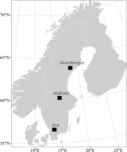
Table 1. Summary statistics for the data set inventoried in 2002, for 31 Norway spruce, 40 Scots pine and 14 birch trees.

Species/Stand	Variables/abbreviations [units]	Mean	Median	Min	Max
Picea abies	dbh [cm]	14.3	12.9	4.2	37.7
	H [m]	11.9	8.9	3.5	27.8
	age [years]	49	43	15	95
	Fresh weight of fractions [kg]	309.5	106.8	8.6	1610.8
Pinus sylvestris	dbh [cm]	21.3	21.3	8.5	39.8
	H [m]	15.5	15.3	6.6	25.5
	age [years]	65	59	20	117
	Fresh weight of fractions [kg]	375.9	312.3	17.4	1332.2
Betula sp.	dbh [cm]	11.9	11.5	5	26.7
	H [m]	11.3	11.1	1.7	20.8
	age [years]	30	29	7	59
	Fresh weight of fractions [kg]	207.8	71.7	0.6	809.4
Stand	Altitude/Alt [m a.sl]	225	211	170	314
	Basal area/Bas [m^2ha^−1]	25	26	12	36
	Basal area-weighted average height/Hbaw [m]	17	17	7	24
	Basal area-weighted average stand age/Agebaw [years]	64	60	30	116
	Site index according to site factors/ SIS [m]	23	22	14	35

Sample tree selection, destructive measurements and carbon concentration determination

On each plot, sample trees were selected by a stratified random procedure. All trees on the plot were callipered at breast height (1.3 m from the ground), numbered and organised in the following diameter classes: 0–10, 10.1–20.0, 20.1–30.0, and 30.1 cm and more. Within each diameter class, one sample tree was selected by simple random sampling if existing. The motivation behind this was facilitated by the allocated budget and the focus was to distribute the sample selection in such a way as to cover many plots, stands and sites rather than sampling many individuals from each diameter class in a single plot. In total, 900 trees were inventoried on all plots and sites. From these, 85 trees (40 pines, 31 spruces and 14 birches) were sub-sampled for felling. The distribution of sample trees per species in 10 cm diameter classes is shown in Figure A1 (see Appendix).

The sample trees were felled following the methodology by Marklund (1987), which meant that a wire was attached to the tree a few metres up on the stem. The other end of the wire was anchored about 40 m away. The attachment of a wire ensured that the whole tree was felled as carefully as possible and in a manner that allowed direct access to the entire tree’s rooting system. All broken branches and twigs longer than 10 cm were gathered together. Living and dead branches were cut off and put into different piles. Each felled tree was divided into components and the total fresh weight was measured for the following tree components; stem including bark, living branches including bark and needles/ leaves, dead branches with bark if bark existed, roots <0.5 cm (in “diameter”), roots 0.5–2 cm, roots >2 cm, and stump. The stems and branches were weighed using specially designed portable weighing equipment. This equipment made it possible to weigh entire stems without cutting them into smaller sections. As the measurement accuracy depends mainly on the maximum capacity of the scale, a set of scales with capacities from five to 500 kg was used to keep measurement errors down. Weights below one kg were measured on an electronic scale with an accuracy of 0.1 g.

For each tree component, sub-samples (about 2–5% depending on the uniformity of the component) were taken and sent to the laboratory for dry weight estimation. If the total fresh weight of the tree was less than 3 kg, no subsampling was done and all of the components were sent to the laboratory. If the diameter at breast height was 10 cm or more, a systematic sample of four stem disks (denoted as 1, 2, 3, and 4 – after standard assortment into timber and pulpwood) was taken. The stem was divided into four sections of equal length and the location of the sample in the first section was randomly selected. The sub-samples of the stem component were scattered along the entire stem but mostly included cross-sections at the stump and breast height. If the diameter of the tree was less than 7 cm, the disks were replaced by two sections, 10–20 cm in length. This was done to avoid high measurement errors due to low sample weights (Marklund 1987).

Up to eight living branches were taken systematically along the crown, and the raw weight was measured. From these, sub-samples constituting about 2% of the fresh weight measured living branches were sent to the laboratory. The dead branches constituted a small and heterogeneous part of the crown, and it was therefore not considered worthwhile to develop any sophisticated sampling procedure for this component. Sub-samples were also taken from roots <0.5 cm, roots 0.5–2 cm, roots >2 cm, and stumps, and sent to the laboratory.

At the laboratory, all samples were oven-dried at 85° Celsius for 48 h, as some tests showed that the samples had then reached constant weight. The dry weights of the samples were measured at the laboratory using the Mettler PE 4000 electronic balance with an accuracy of 0.1 g. The dry weights of the samples were determined immediately after they were taken out from the drying chamber (otherwise they would quickly absorb moisture from the air). The C concentration in the samples was measured using nearly 600 ground sub-samples (283 subsamples of stems, 108 subsamples of branches with needles/ leaves, and 188 subsamples of stumps with roots) and using the “flash combustion method” with the Nitrogen Analyzer NA 1500 (Verardo et al. 1990).

To facilitate the application of the C concentration estimates to the different pools of biomass in Sweden (Marklund, 1987; Petersson and Ståhl 2006), three groups of tree carbon components were created by combining (1) stem and bark, (2) branches and needles, and (3) stumps and roots.

Inference of whole-tree mean carbon concentration

In the present study, the trees were considered as the sampling units. To estimate the C concentration of whole trees, utilising random samples from different tree components, the size of the tree components must be considered with weighting. Weighting is also important, for example, when large trees are compared with small ones because the trunk's relative share of the whole tree increases with tree size (and age). Therefore, the C concentration per sample was weighted against the measured total raw/fresh weight per tree component (Equation 1) following Everitt and Skrondal (2010). (1) ${\hat{\mu }}_{\mathrm{cc}}={\displaystyle \frac{{\sum }_{i=1}^n{x}_i\cdot w_i}{{\sum }_{i=1}^n{w}_i}}$(1) (2) $s_{{\hat{\mu }}_{\mathrm{cc}}}=\sqrt{{\displaystyle \frac{{\sum }_{i=1}{w}_i\cdot {(x_i-{\hat{\mu }}_{\mathrm{cc}})}^2}{{\displaystyle \frac{(n^{\mathrm{\prime }}-1)\cdot {\sum }_{i=1}{w}_i}{n^{\mathrm{\prime }}}}}}}$(2) where ${\hat{\mu }}_{\mathrm{cc}}$ is the weighted mean C concentration (%) at the tree or component level, $s_{{\hat{\mu }}_{\mathrm{cc}}}$ is the weighted standard deviation of ${\hat{\mu }}_{\mathrm{cc}}$, $x_i$ is the measured individual component or tree-level C concentration (%), $w_i$ is the raw weight for the i^th fraction over trees, $n$ is the number of observations and $n^{\mathrm{\prime }}$ is the number of non-zero raw weights of fractions. The standard deviation was converted to standard error by adjusting for sample size.

Inference of C concentration was made for the following strata; whole tree, components (stemwood and bark, living branches and needles/ leaves, and stumps and roots), species (birch, spruce, and pine), and region (Asa, Jädraås, and Svartberget). For spruce, the measurements in Flakaliden (only 3 trees) were combined with those from Svartberget.

To infer the average C concentration of trees on all forestland (including protected areas) in Sweden, we used the recent 5-year observations of total biomass made by the Swedish National Forest Inventory (NFI). Data corresponding to the surveys of 2018–2022 and the major tree species (pine, spruce and birch) were used for the analyses. Detailed information (e.g. sampling, response and estimation designs) about the Swedish NFI can be found in Fridman et al. (2014). The population-level weighted average C (${\hat{\mu }}_p$) was evaluated for each species and combined species as follows: (3) ${\hat{\mu }}_p=\sum {\displaystyle \frac{{\hat{\mu }}_{\mathrm{cc}}\cdot T{B}_i}{\mathrm{TB}}}$(3) where ${\hat{\mu }}_{\mathrm{cc}}$ is derived from Equation 1, $T{B}_i$ is the total biomass (in a million tonnes) for species $i$, and $\mathrm{TB}$ is the total biomass for all species combined.

Statistical analyses

The statistical analyses were conducted in R (R Core Team 2022) and mainly involved analysis of variance (ANOVA) tests using the “rstatix” package and linear mixed-effects regression from the “lme4” package. Before the ANOVA tests, initial assumptions on the distribution (i.e. normality) and sphericity (i.e. variance homogeneity) of the response variable (C concentration) were investigated. Normality was verified statistically by the Shapiro–Wilk test, and by visual inspection using quantile-quantile plots (not presented in the study). Significant tests were made at a 5% alpha level. Where there was a significant difference, the Bonferroni multiple testing correction method was used for pairwise comparison.

To examine whether the observed average C concentration differed among pine, spruce and birch (objective 1); we employed the one-way ANOVA test. The F-test statistic (derived as the ratio of between-group variation to within-group variation, assuming the statistic follows the F-distribution) was used to examine statistically (by comparing with the critical F value at a 5% significance level) if the average C concentration was significantly different among tree species.

To determine whether the average C concentration differed among tree components (objective 2) and along the stem (objective 3) for a given species; we used the test of repeated-measures ANOVA. The repeated-measures ANOVA test was chosen because the same individuals were measured on the same C concentration under different tree components (i.e. branches, stemwood and stumps). We quantified the amount of variability due to the within-component factor through the generalised effect size estimator (${\eta }_g^2$).

To investigate the influence of tree and stand characteristics on the expected C concentration in the tree fractions (objective 4), we used a linear mixed-effects regression model. For a given component and tree, sub-samples were pooled together to obtain the average C concentration and the model fit was done separately for the three tree fractions. The mixed model was considered appropriate due to the hierarchical structure of the data (i.e. observations from trees nested within sample plots). We used a mixed-effects regression model with two-level random groups (Equation 4) to study the random effects for plot and trees in a plot as: (4) $y_{\mathrm{ij}}=x_{\mathrm{ij}}\beta +{\alpha }_i+{\gamma }_{\mathrm{ij}}+{ϵ}_{\mathrm{ij}}$(4) where $y_{\mathrm{ij}}$ is the carbon concentration of tree $j$ of plot $i$, $x_{\mathrm{ij}}\beta$ represents the fixed part of the model with $x_{\mathrm{ij}}$ describing the influence of tree (e.g. species, diameter, age, and health) and stand (e.g. site index, basal area, height, soil type) characteristics on the average C concentration of tree $j$ of plot $i$. $\beta$s are parameters to be estimated from the sample data, ${\alpha }_i$ is the random effect for plot $i$, ${\gamma }_{\mathrm{ij}}$ is the random effects for tree $j$ of plot $i$, and ${ϵ}_{\mathrm{ij}}$ is the residual error. The random effects are normally distributed and independent across plots and residual errors are independent across observations. However, preliminary analysis showed that the residuals have increasing variance. Therefore, a power variance function with two parameters (scale and shape, denoted as ${\omega }^2$ and ${\delta }_1$, respectively) (Equation 5) was used to account adjust the heteroscedastic effect. (5) $V({ϵ}_{\mathrm{ij}})={\omega }^2|\widehat{y_{\mathrm{ij}}}{|}^{2{\delta }_1}$(5) Due to the reason that biometric information on tree stems (e.g. stem diameter at breast height) is easily obtained and readily available in most forest inventories compared to difficult-to-measure parameters such as stumps, roots, and branches, we examined whether the concentration of C in stemwood could provide a good direct approximation for the C concentration of other tree components such as branches and stumps. We compared and quantified the agreement between the measured C concentrations for the same trees where the C concentration was measured in the stemwood, branches, and stumps. The C concentration of stemwood served as the reference in all the comparisons. Thus, we compared separately the C concentrations between stemwood and stumps and between stemwood and branches. Following the approach proposed by Bland and Altman (1999), the agreement in C concentrations between the compared components was studied by quantifying the differences in C concentrations between observations and estimating the 95% confidence limits of agreement (based on ±1.96 standard deviation of the mean difference) as a measure of uncertainty around the mean difference. Further, we used a one-sample t-test to examine statistically if the mean difference (${\mu }_d$) for the compared components was significantly different from zero (at a 5% alpha level). An observed difference not significantly different from zero (p > 0.05) suggested the stemwood C concentration value might be a suitable proxy for whole tree C inference and otherwise.

Results

Table 2 shows the average C concentration for each tree species, fraction, and region. The whole tree average C concentration (%) differed significantly between tree species (F_{(2, 68)} = 11.72, p < 0.0001). The results from the pairwise comparison t-tests showed that the average C concentration (mean ± standard error) of Scots pine was higher (50.671 ± 0.211) than in Norway spruce (49.518 ± 0.164) and birch (49.347 ± 0.241). However, the two latter tree species had similar C concentrations (Figure 2). As an average for all tree species and regions, the C concentration was estimated as 50.184 ± 0.189 (Table 2).

Figure 2. Variation in the average tree-level C concentration of different tree species. Results from the ANOVA test (the F-test statistic and the p-value) are presented along with multiple pairwise paired t-tests between the different tree species (ns = not statistically significant, ** and *** show significant differences with adjusted p-values 0.01 < p < 0.001 and p < 0.001, respectively). The amount of variation within species (${\eta }_g^2$) was 26%. The boxplot shows the mean (red dots), the median (horizontal lines) and the 25th and 75th quartiles.

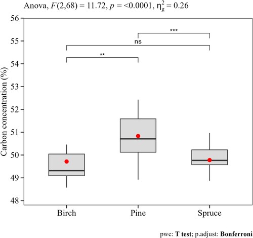
Table 2. Tree-level average (± standard error) C concentration (%) per species and components at different areas.

Species	Component	Asa	Jädraås	Svartberget	All sites
Birch	Branches	50.144 ± 0.699	51.681 ± 0.394	49.845 ± 0.673	50.556 ± 0.328
	Stemwood + bark	48.602 ± 0.251	49.662 ± 0.132	49.398 ± 0.201	49.221 ± 0.109
	Stump + roots	48.888 ± 0.743	49.387 ± 0.134	48.538 ± 0.642	49.938 ± 0.287
	Whole tree	48.891 ± 0.564	49.993 ± 0.221	49.157 ± 0.505	49.347 ± 0.241
Spruce	Branches	50.540 ± 0.415	51.076 ± 0.689	49.914 ± 0.269	50.511 ± 0.253
	Stemwood + bark	49.131 ± 0.078	48.965 ± 0.454	49.066 ± 0.099	49.054 ± 0.111
	Stump + roots	50.159 ± 0.216	50.019 ± 0.319	49.143 ± 0.149	49.774 ± 0.129
	Whole tree	49.652 ± 0.236	49.703 ± 0.487	49.201 ± 0.172	49.518 ± 0.164
Pine	Branches	54.353 ± 0.789	51.505 ± 0.249	51.808 ± 0.423	52.555 ± 0.223
	Stemwood + bark	50.061 ± 0.083	50.739 ± 0.451	50.104 ± 0.192	50.301 ± 0.225
	Stump + roots	51.299 ± 0.056	50.499 ± 0.437	50.580 ± 0.351	50.793 ± 0.184
	Whole tree	50.733 ± 0.309	50.847 ± 0.379	50.430 ± 0.322	50.671 ± 0.211
All species, sites and components combined			50.184 ± 0.189

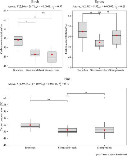
Within species, the mean C concentration differed between tree components (Figure 3). Branches had higher C concentration values than stemwood (with bark) and stumps (with roots) components. For example, the mean C concentration in the branches of pines at all sites was 52.555% (Table 2). Using a C concentration value of 50% would thus result in an underestimation of 4.86% of the C concentration.

Figure 3. Variation in C concentration among tree components. Results from the ANOVA test (the F-test statistic and the p-value) are presented along with multiple pairwise paired t-tests between the different tree components (ns = not statistically significant, ** and *** show significant differences with adjusted p-values 0.01 < p < 0.001 and p < 0.001, respectively). The amount of variability due to the within-fraction factor (${\eta }_g^2$) was 57%, 21% and 19% respectively for birch, spruce and pine. The boxplot shows the mean (red dots), the median (horizontal lines) and the 25th and 75th quartiles.

Across sites, the C concentrations in tree components showed a latitudinal trend. Generally, the C concentrations decreased from Svartberget in the north to Asa in the south of Sweden, though the differences between sites appear to be small. The conifers (pine and spruce) had higher C concentrations than birch in all three sites (Table 2).

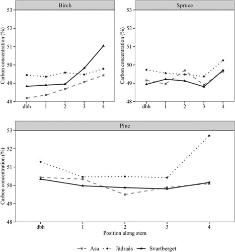
The C concentration along the stemwood with bark was analysed per species and region. In general, the C concentration showed a tendency to increase along the stem, however, measurements at higher stem positions did not differ significantly (p > 0.05) from those measured at breast height (Figure 4).

Figure 4. Average C concentration at breast height (dbh – 1.3 m from the ground), and other four locations (1, 2, 3, 4) systematically scattered along the stem after standard assortment (i.e. timber and pulpwood).

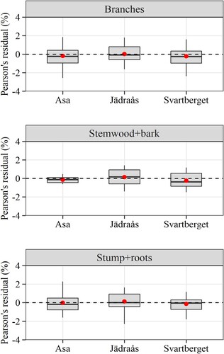
To determine whether the C concentration in the various tree components is dependent on tree size, stand structure, and other site characteristics, analyses using linear-mixed effects models were carried out. Table 3 shows the estimated parameters of the regression model for each component. Only tree species identity had a significant effect on the C concentration in all tree components. The estimated random effects for plots and trees in a plot were minimal in each component. Besides, Pearson’s residuals did not show heteroscedasticity across regions (Figure A2), indicating that the error variance was satisfactorily modelled by the power function.

Table 3. Parameter estimates of the mixed model (Equation 4(4) $y_{\mathrm{ij}}=x_{\mathrm{ij}}\beta +{\alpha }_i+{\gamma }_{\mathrm{ij}}+{ϵ}_{\mathrm{ij}}$(4) ) describing the effects of tree, stand, and site characteristics on the C concentration of branches, stemwood and stumps.

		Fixed component
		Branches	Stemwood + bark	Stump + roots
	Predictors	Coefficient	Coefficient	Coefficient
Source	Intercept	52.098 (2.144)	50.334 (1.249)	47.496 (1.578)
Tree	Species	1.322 (0.677)	1.712 (0.434)	1.477 (0.539)
Tree	dbh	0.001 (0.004)	0.002 (0.003)	−0.0007 (0.0034)
Tree	Age	−0.012 (0.014)	−0.021 (0.009)	0.004 (0.011)
Tree	Id-5	−0.036 (0.082)	−0.013 (0.048)	−0.013 (0.064)
Tree	Tree health	−0.560 (0.625)	−0.562 (0.368)	−0.271 (0.424)
Site	SIS	−0.033 (0.079)	−0.037 (0.047)	0.122 (0.058)
Stand	Bas	0.0004 (0.041)	0.004 (0.026)	0.003 (0.031)
Stand	H-baw	0.025 (0.066)	0.038 (0.041)	−0.062 (0.054)
Site	Soil type	0.372 (0.464)	0.364 (0.341)	0.165 (0.410)
Random component
	$\widehat{\mathrm{var}}({\alpha }_i)$	5.123 × 10^−13	4.480 × 10^−14	3.473 × 10^−11
	$\widehat{\mathrm{var}}({\gamma }_{\mathrm{ij}})$	1.668 × 10^−15	3.889 × 10^−14	1.101
Residual variance $\hat{V}({ϵ}_{\mathrm{ij}})$
	$\hat{\omega }$	1.604 × 10^−14	9.015 × 10^−14	2.483 × 10^−5
	${\hat{\delta }}_1$	8.165	8.560	2.950

Notes: significant variables are highlighted in bold. Variable definitions: Id-5 is a 5-year diameter increment, soil type is an indicator for either moraine (1) or peat soil (0); Tree health is a binary variable where 1 is undamaged, otherwise 0 for damaged trees. Other variables are already defined (see Table 1). The estimated random variances are given in standard deviations.

Values in parentheses are standard errors of the estimates. Significant variables are highlighted in bold.

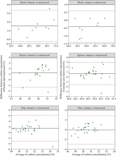
The comparisons between C concentrations of stemwood and other tree components showed heterogeneous outcomes (Figure 5). In all compared components, the 95% confidence intervals of the mean differences (${\mu }_d$) were wider; suggesting large uncertainties in the agreements between C concentrations in the stemwood and branches and stumps. In addition, except for the stump and stemwood C concentrations of pine (${\hat{\mu }}_d$ = −0.057, t-test static = −0.204, df = 27, p-value = 0.839), the results from the one-sample t-test showed that the mean difference (${\mu }_d$) in C concentrations was significantly different from zero for all species in the comparisons of stemwood versus stump (spruce: ${\hat{\mu }}_d$ = 0.683, t-test static = 2.941, df = 27, p-value = 0.007; birch: ${\hat{\mu }}_d$ = −0.401, t-test static = −2.345, df = 8, p-value = 0.047) and the stemwood versus branches (pine: ${\hat{\mu }}_d$ = 1.489, t-test static = 3.154, df = 27, p-value = 0.004; spruce: ${\hat{\mu }}_d$ = 1.244, t-test static = 4.1208, df = 18, p-value = 0.001; birch: ${\hat{\mu }}_d$ = 1.556, t-test static = 5.043, df = 8, p-value = 0.001). Thus, the observed results generally imply that the C concentration value in stemwood may not be a suitable proxy for inference of the C concentrations in the stumps and branches of trees in Swedish forests.

Figure 5. The Bland-Altman plot of agreement between C concentrations of branches, stumps and stemwood for birch, spruce and pine. The y and x axes show the difference and average C concentrations between the compared components (stemwood versus stumps and stemwood versus branches). The black (solid) lines represent the average difference in C concentration between branch and stemwood (left panel) and stump and stemwood (right panel). The dashed (red) lines represent the 95% confidence intervals of agreement.

To infer the average C concentration of trees on all forestlands (including protected areas) in Sweden, we applied the species and component-specific C constants obtained in Table 2 to the latest observations (2018–2022) of total biomass from the Swedish NFI. We found that the average C concentration of trees (pine, spruce and birch) was 50.012% (Table 4).

Table 4. Total biomass (million tonnes) and average weighted carbon (C) concentration (%) per species and components for all trees on Forestlands inventoried by the Swedish NFI in the period 2018–2022.

Species	Stem and bark	Branches and needles	Stump and roots	Weighted C content, ${\hat{\mu }}_p$
Scots pine	562.260	137.902	232.662	50.757
Norway spruce	550.963	268.727	272.575	49.592
Birch	244.412	67.709	107.597	49.620
All species	1357.635	474.338	612.833	50.012

Discussion

To represent a latitudinal gradient in C concentration, three regions (sites) were chosen subjectively. Within sites, stands were selected subjectively. Thus, the data do not represent the C concentration of Swedish trees but a subjective sample of Swedish forests. Within stands, plots were randomly selected and trees were randomly sampled within plots. There are probably dependencies within plots and especially within trees, which may affect statistical test quantities. These dependencies should falsely strengthen differences between sites, but despite this, differences in C concentrations were small between tree species, within tree species, and by latitude (Figures 2 and 3, Table 2). The dependencies were addressed statistically in two main ways. First, we used repeated measures ANOVA to evaluate the within-component C differences. This method accounted for the effect of having correlated observations on the same sampling unit (i.e. branch, stem, and stump C concentrations measured on the same sample tree). The generalised effect size (${\eta }_g^2$) expressing the amount of variability due to the within-fraction group indicated a higher variance for birch (Figure 3). Second, we used linear mixed-effects regression with two-level random groups to account for the dependencies of trees within plots and between plots. The variance estimates were smaller between plots than between trees in a plot (Table 3).

The average C concentration (%) value for all species combined was 50.184 ± 0.189. This value is similar to the nominal value of 50% assumed in most global tree carbon assessment studies (e.g. Ladanai et al. 2010; Thomas and Martin 2012; Strömgren et al. 2013) but higher than the general “default value” of 47% C suggested by the IPCC (IPCC 2006). However, the observed differences in Table 2 suggest that accurate information on species- and component-specific differences may substantially reduce the error associated with biomass-carbon conversions by ∼ 2.5–3.7% (Thomas and Martin 2012). Further, we observed that only species affected the C concentration significantly in each component (Table 3). The conifers, pine (50.671 ± 0.211), and spruce (49.518 ± 0.164) had on average higher C concentrations than birch (49.347 ± 0.241). This finding was also reported by Ma et al. (2018) and the explanation for this is probably the higher relative degree of lignification of tissues in conifers compared to broadleaves (Minami and Saka 2003). Within species, the average C concentration differed between components. The branch components had higher C concentration than those of stemwood with bark and stump with roots (Figure 3). In our study, the C analysis was made for combined stemwood and bark; however, earlier studies indicated a significantly higher C concentration in the bark (56.2%) than in the stemwood (50.5%) for major boreal tree species including pine and spruce (Gao et al. 2016). The difference between bark and stemwood C is mainly the amount of volatile carbon present in the components . The average volatile C for boreal species is about 5.8% in the bark and 3% in the stemwood (Gao et al. 2016).

In earlier reports, analyses of component-specific wood C values indicated that stemwood C provides a good direct approximation for C concentration in other tree components (Thomas and Martin 2012). However, our results provided heterogeneous conclusions (Figure 5). Martin et al. (2013) suggested that volatile C might influence size-associated changes in the total C concentration by offsetting size-related decreases in C-rich lignin. Gao et al. (2016) found significant and positive relationships between stemwood C concentration and diameter at breast height for shade-intolerant boreal species, whereas those of shade-tolerant species showed negative or neutral size-associated change. The explanation for the positive size-associated trend may be related to a shift in allocation to secondary volatile C compounds to support defence functions (Gao et al. 2016). Thus, the insignificance of age and diameter on the observed C concentration in our study may be perhaps attributed to the omission of volatile C during the elementary analysis.

The discrepancies in C concentration between fractions and species are often a result of the measurement technique and elementary analysis of carbon (Thomas and Martin 2012). For example, the widely used “flash combustion method” where the C concentration is estimated at a constant dry weight temperature of 85°C means that the compounds (such as alcohols, phenols, terpenoids, and aldehydes) may be volatilised even before the elemental analysis (Lamlom and Savidge 2003; Thomas and Martin 2012; Gao et al. 2016). Generally, the problem may be alleviated by applying a “carbon conversion factor” that corrects for mass and C loss during sample drying (Martin and Thomas 2011). In the present study, we used the flash combustion method and elementary analysis of the dry-weight samples. These may introduce additional errors in our estimates. Therefore, we suggest future studies to investigate the magnitude of the errors and their impacts on carbon accounting in the Swedish forests.

Conclusion

This paper examined empirically the average C concentration of the major tree species (pine, spruce, and birch) in Swedish forests along a latitudinal gradient. The following conclusions were drawn: (1) the average C concentration value (%) for all tree species combined was 50.184 ± 0.189. (2) It is better to use different constants per species and maybe per species and component as provided in Table 2. (3) No need to consider the latitude, tree size, age, growth, etc. when estimating the C concentration of the major tree species. (4) It is uncertain that a high C concentration in the stem also indicates a high C concentration in other tree components such as branches, stumps, and roots. (5) By applying the species- and component-specific weighted C constants to the latest observations of total biomass from the Swedish National Forest Inventory, we found that the average C concentration of trees (pine, spruce and birch) in all forestlands was approximately 50.012% in Sweden. Our results potentially contribute to the need for accurate reporting of C sequestration in the sector of Land Use, Land Use Change and Forestry.

Credit authorship contribution statement

Alex Appiah Mensah: Conceptualization, Methodology, Data curation, Formal analysis, Writing – original draft, Writing – review & editing. Hans Petersson: Conceptualization, Methodology, Data curation, Writing – original draft, Writing – review & editing, Funding acquisition, Supervision.

Acknowledgements

The Swedish Environment Protection Agency financially supported this study through the project “International Reporting of Greenhouse Gas Emissions from the LULUCF Sector” (grant number 74426005).

Data availability

Data will be made available on request.

Disclosure statement

No potential conflict of interest was reported by the author(s).

Additional information

Funding

This work was supported by Naturvårdsverket [grant number 74426005].

Appendix

Figure A1. The number of trees per species inventoried on all plots and sites (A) and the sub-sampled trees for destructive measurements (B) in 10 cm diameter classes.

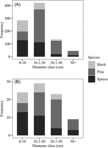
Figure A2. Residual distribution over sites. The residuals are from the mixed-effects linear regression model describing the effects of tree, stand and site characteristics on the average carbon concentration in tree components.

References

- Alriksson A, Eriksson HM. 1998. Variations in mineral nutrient and C distribution in the soil and vegetation compartments of five temperate tree species in NE Sweden. For Ecol Manag. 108:261–273. doi:10.1016/S0378-1127(98)00230-8.
- Bert D, Danjon F. 2006. Carbon concentration variations in the roots stem and crown of mature Pinus pinaster (Ait.). For Ecol Manag. 222:279–295. doi:10.1016/j.foreco.2005.10.030.
- Bland JM, Altman DG. 1999. Measuring agreement in method comparison studies. Stat Methods Med Res. 8(2):135–160. doi:10.1177/096228029900800204.
- Everitt BS, Skrondal A. 2010. The Cambridge dictionary of statistics. Fourth Edition. Cambridge University Press, New York, United States of America.
- Fridman J, Holm S, Nilsson M, Nilsson P, Ringvall AH, Stahl G. 2014. Adapting National Forest Inventories to changing requirements - the case of the Swedish National Forest Inventory at the turn of the twentieth century. Silva Fenn. 48:1095. doi:10.14214/sf.1095.
- Gao B, Taylor AR, Chen HYH, Wang J. 2016. Variation in total and volatile carbon concentration among the major tree species of the boreal forest. For Ecol Manag. 375:191–199. doi:10.1016/j.foreco.2016.05.041.
- IPCC. 2006. Forest lands, Vol. 4. Hayama, Japan: Intergovernmental Panel on Climate Change Guidelines for National Greenhouse Gas Inventories; Institute for Global Environmental Strategies (IGES). p. 83.
- Ladanai S, Ågren GI, Olsson BA. 2010. Relationships between tree and soil properties in Picea abies and Pinus sylvestris forests in Sweden. Ecosystems. 13:302–316. doi:10.1007/s10021-010-9319-4.
- Lamlom SH, Savidge RA. 2003. A reassessment of carbon content in wood: variation within and between 41 North American species. Biomass Bioenergy. 25:381–388. doi:10.1016/S0961-9534(03)00033-3.
- Ma S, He F, Tian D, Zou D, Yan Z, Yang Y, Zhou T, Huang K, Shen H, Fang J. 2018. Variations and determinants of carbon content in plants: a global synthesis. Biogeosciences. 15:693–702. doi:10.5194/bg-15-693-2018.
- Marklund LG. 1987. Biomass functions for Norway spruce (Picea abies [L.] Karst.) in Sweden [biomass determination, dry weight]. Rapport-Sveriges Lantbruksuniversitet, Institutionen För Skogstaxering (Sweden).
- Martin AR, Gezahegn S, Thomas SC. 2015. Variation in carbon and nitrogen concentration among major woody tissue types in temperate trees. Can J For Res. 45:744–757. doi:10.1139/cjfr-2015-0024.
- Martin AR, Thomas SC. 2011. A reassessment of carbon content in tropical trees. PLoS One. 6:e23533. doi:10.1371/journal.pone.0023533.
- Martin AR, Thomas SC. 2013. Size-dependent changes in leaf and wood chemical traits in two Caribbean rainforest trees. Tree Physiol. 33:1338–1353. doi:10.1093/treephys/tpt085.
- Martin AR, Thomas SC, Zhao Y. 2013. Size-dependent changes in wood chemical traits: a comparison of neotropical saplings and large trees. AoB Plants. 5:plt039. doi:10.1093/aobpla/plt039.
- Minami E, Saka S. 2003. Comparison of the decomposition behaviours of hardwood and softwood in supercritical methanol. J Wood Sci. 49:0073–0078. doi:10.1007/s100860300012.
- Petersson H, Ståhl G. 2006. Functions for below-ground biomass of Pinus sylvestris, Picea abies, Betula pendula and Betula pubescens in Sweden. Scand J For Res. 21:84–93. doi:10.1080/14004080500486864.
- R Core Team. 2022. R: a language and environment for statistical computing. Vienna, Austria: R Foundation for Statistical Computing. https://www.R-project.org/
- Strömgren M, Egnell G, Olsson BA. 2013. Carbon stocks in four forest stands in Sweden 25 years after harvesting of slash and stumps. For Ecol Manag. 290:59–66. doi:10.1016/j.foreco.2012.06.052.
- Thomas SC, Martin AR. 2012. Carbon content of tree tissues: a synthesis. Forests. 3:332–352. doi:10.3390/f3020332.
- Verardo DJ, Froelich PN, McIntyre A. 1990. Determination of organic carbon and nitrogen in marine sediments using the Carlo Erba NA-1500 analyzer. Deep Sea Res A. 37:157–165. doi:10.1016/0198-0149(90)90034-S.