Zonostrophic instabilities in magnetohydrodynamic Kolmogorov flow

Abstract

A classic stability problem relevant to many applications in geophysical and astrophysical fluid mechanics is that of Kolmogorov flow, a unidirectional purely sinusoidal velocity field written here as $\mathit{u}=(0,\sin x)$ in the infinite $(x,y)$-plane. Near onset, instabilities take the form of large-scale transverse flows, in other words flows in the x-direction with a small wavenumber k in the y-direction. This is similar to the phenomenon known as zonostrophic instability, found in many examples of randomly forced fluid flows modelling geophysical and planetary systems. The present paper studies the effect of incorporating a magnetic field $B_0$, in particular a y-directed “vertical” field or an x-directed “horizontal” field. The linear stability problem is truncated to determining the eigenvalues of finite matrices numerically, allowing exploration of the instability growth rate p as a function of the wavenumber k in the y-direction and a Bloch wavenumber ℓ in the x-direction, with $-1/2<\ell \le 1/2$. In parallel, asymptotic approximations are developed, valid in the limits $k\to 0$, $\ell \to 0$, using matrix eigenvalue perturbation theory. Results are presented showing the robust suppression of the hydrodynamic Kolmogorov flow instability as the imposed magnetic field $B_0$ is increased from zero. However with increasing $B_0$, further branches of instability become evident. For vertical field there is a strong-field branch of destabilised Alfvén waves present when the magnetic Prandtl number $P_m<1$, as found recently by A.E. Fraser, I.G. Cresswell and P. Garaud (J. Fluid Mech. 949, A43, 2022), and a further branch for $P_m>1$ in the presence of an additional imposed x-directed fluid flow $U_0$. For horizontal magnetic field, a branch of field-driven, tearing mode instabilities emerges as $B_0$ increases. The above instabilities are present for Bloch wavenumber $\ell =0$; however allowing ℓ to be non-zero gives rise to a further branch of instabilities in the case of horizontal field. In some circumstances, even when the system is hydrodynamically stable arbitrarily weak magnetic fields can give growing modes, via the instability taking place on large scales in x and y. Detailed comparisons are given between theory for small k and ℓ, and numerical results.

Keywords:

• Magnetohydrodynamics
• Kolmogorov flow
• zonostrophic instability

1. Introduction

The Kolmogorov flow, a periodic flow forced at a single wavenumber, is a fundamental flow to study owing to its simplicity and its application to a wide range of geophysical and astrophysical systems. Its stability to infinitesimal disturbances is a classic problem first posed by Kolmogorov and studied by Meshalkin and Sinai (1961). These authors made use of continued fraction expansions to establish properties of the growth rate $p(k)$, where k is a wavenumber in the streamwise direction, and determined a critical Reynolds number of ${R_e}_c=\sqrt{2}$. Close to onset of instability, for $R_e$ slightly larger than $\sqrt{2}$, it is large scale modes that are destabilised; more precisely, for $R_e=\sqrt{2}(1+3k^2+\cdots )$ the most unstable mode has wave number $k\ll 1$. This property allows the development of amplitude equations governing the flow on large space and time scales, derived by Nepomniashchii (1976) and Sivashinsky (1985). Numerical simulations by She (1987) showed evolution from the most unstable scale to larger scales via an inverse cascade of vortex pairings, for a large scale allowed only in the y-direction. Here and elsewhere in the present paper and discussion of other authors' work, we adopt the convention of writing the non-dimensional Kolmogorov flow as ${\mathit{u}}_0=(0,\sin x)$ in the $(x,y)$ plane so that y is the streamwise coordinate. For large scales in both x- and y-directions, Sivashinsky (1985) showed evolution to a large-scale flow with chaotic temporal fluctuations, further explored in Lucas and Kerswell (2014, 2015).

The stability problem posed by Kolmogorov is such a basic building block for theory that it has been elaborated in several studies by incorporating further physical phenomena. Frisch et al. (1996) included a β-effect, giving the gradient of a background planetary vorticity distribution; the gradient is oriented along the x direction (again following our conventions rather than those of the original paper), so that it does not interact directly with the basic state Kolmogorov flow ${\mathit{u}}_0$, only on $k\ne 0$ linear modes. These authors derived an amplitude equation near to onset for a large scale in y, which they called the β-Cahn–Hilliard equation. For $\beta =0$ this reduces to the PDE of Sivashinsky (1985) and simulations show that the inverse cascade of structures to large scales in y is arrested by the β-effect. These authors characterise the fundamental instability of the Kolmogorov flow as due to a negative effective viscosity, in other words that the large-scale y-dependent modes have growth rate $p=-{\nu }_E{k}^2+\cdots$ for $k\ll 1$, where the effective viscosity (or eddy viscosity) ${\nu }_E$ changes sign from positive below the threshold $R_{\mathrm{ec}}=\sqrt{2}$, to negative above. This destabilises the flow on large scales with the fastest growing modes determined by the next terms in this series (Dubrulle and Frisch 1991).

In terms of the geophysical motivation for these stability problems, any orientation of the background vorticity gradient, parameterised by β, with respect to the Kolmgorov flow is of interest. Manfroi and Young (2002) allow an arbitrary angle α between flow and gradient in a study of linear stability and nonlinear evolution using amplitude equations generalising those of Sivashinsky (1985) and Frisch et al. (1996). They find that the linear problem shows a delicate dependence of critical Reynolds number on angle α when unstable modes are allowed to adopt arbitrarily large scales in x and y. Another effect of geophysical relevance that may be included is stratification. Balmforth and Young (2002) considered the sinusoidal flow in the $(x,z)$ plane with gravity in the $-z$ direction and the flow directed in x, sinusoidal in z. These authors determined the behaviour of linear instabilities, depending on Reynolds, Richardson and Prandtl numbers, and derived an amplitude equation generalising that of Sivashinsky (1985). Simulations show that the inverse cascade of She (1987) is arrested by the presence of stratification over a wide range of parameters.

Relevant to the present paper, in astrophysical applications it is natural to introduce a magnetic field and study the coupled MHD system; as general motivation we note, for example, that the interaction between magnetic field, shear, and convection remains poorly understood in the solar tachocline (Hughes et al. 2007). Boffetta et al. (2000) considered the case in which a sinusoidal magnetic field (maintained by a source term in the induction equation) sits in a motionless fluid. This magnetic Kolmogorov system shows instabilities and an amplitude equation gives an inverse cascade to large scales. Related work concerns the tearing mode instability (Boldyrev and Loureiro 2018) and parasitic modes for magnetorotational instabilities, the latter involving a basic state of both sinusoidal magnetic and flow fields (e.g. Pessah 2010). The recent paper Fraser et al. (2022) considers a background uniform magnetic field ${\mathit{B}}_0=(0,B_0)$ that is aligned with the Kolmogorov flow; this has no effect on the basic state flow but the elasticity of field lines affects perturbations depending on y, through the Lorentz force. These authors observe magnetic suppression of the hydrodynamic instability first analysed by Meshalkin and Sinai (1961), as one might intuitively expect, but also two new families of unstable modes which only exist in the presence of magnetic field. One family exists when the magnetic Prandtl number $P_m<1$, for arbitrarily strong magnetic fields, provided the Reynolds number is above a threshold depending on $P_m$. Here $P_m$ is defined by $P_m=R_m/R_e$, where $R_e$ is the Reynolds number as above and $R_m$ the magnetic Reynolds number. This family is studied numerically and growth rates obtained through asymptotic approximations for $k\ll 1$; these authors refer to the modes as Alfvén Dubrulle–Frisch modes, as the instability can again be linked to a change of sign of the effective viscosity ${\nu }_E$ (Dubrulle and Frisch 1991). The recent thesis of Lewis (2022) considers instabilities of a basic state of a fluid shear layer or jet $(0,u(x))$, with a transverse magnetic field $(B_0,b(x))$, shaped by the fluid flow. Purely hydrodynamic instability of the layer or jet tends to be suppressed by weak magnetic field, while for strong fields, instabilities become magnetically driven.

Study of Kolmogorov flow instabilities is relevant to the formation of zonal flows in forced fluid systems, so-called “zonostrophic instability” (Galperin et al. 2006). This process of jet formation has now been observed in many simulations, observations and experiments; see the representative studies: Vallis and Maltrud (1993), Read et al. (2007), Farrell and Ioannou (2008), Scott and Dritschel (2012), Srinivasan and Young (2012), Bouchet et al. (2013), Parker and Krommes (2014), Lemasquerier et al. (2023), and the book Galperin and Read (2019). Related to our work, Tobias et al. (2007) incorporated a magnetic field aligned with the x-direction of a planar fluid system with a β-effect present, a vorticity gradient in y (extended to spherical geometry in Tobias et al. 2011). The system was driven by a body force with a given characteristic spatial scale. These authors observed the formation of jets in the x-direction for zero magnetic field, but then the suppression of jets, even at quite weak field strengths $B_0$. For fixed non-dimensional β, forcing and viscosity $\nu ={10}^{-4}$, this process was explored by means of a series of runs with varying magnetic field strength $B_0$ and magnetic diffusivity η, and evidence for a threshold scaling law of $B_0^2\sim \eta$ was observed. Constantinou and Parker (2018) analysed Kelvin–Orr shearing wave dynamics for Rossby/Alfvén waves and the interplay between Reynolds and Maxwell stresses, providing evidence for this $B_0^2\sim \eta$ threshold for jet formation. Durston and Gilbert (2016) focused on the couplings between large-scale zonal flow and zonal field in the presence of waves, calculating an effective viscosity and effective magnetic diffusivity, plus an effective cross transport term in which current gradients can drive the zonal vorticity; this and other transport effects are discussed in Chechkin (1999), Kim (2007), and Leprovost and Kim (2009). Parker and Constantinou (2019) interpret the presence or otherwise of jets in terms of the competition between a positive magnetic effective diffusivity term and a negative, purely hydrodynamic effective viscosity. Note that while these studies of zonostrophic instability have many qualitative features in common with the topic of Kolmogorov flow instability, there are key differences that make any direct comparison difficult, even of scaling laws. The reason is that the studies referred to in this paragraph use a forcing which has a given spatial scale but is random in time, and it is the statistics and strength of the forcing that are kept fixed while other parameters, such as the viscosity, magnetic diffusivity, magnetic field and β, are varied. In non-dimensional terms, the key control parameter is a Grashof number (formed from forcing strength, length scale and viscosity) in these systems (Childress et al. 2001, Durston and Gilbert 2016). The Reynolds number is then a diagnostic parameter, and can vary considerably in different regimes depending on the dominant balances in the Navier–Stokes equation between the forcing term, inertial term, viscous term and Lorentz force. However for stability of Kolmogorov flow, the basic state is fixed while the forcing is adjusted to maintain this: the control parameter is a Reynolds number instead.

In the present paper we return to the classic set-up of steady, planar, Kolmogorov flow ${\mathit{u}}_0=(0,\sin x)$ and consider the effect on its stability from magnetic field in the x- and y-directions. We find it convenient to refer to magnetic field in the y-direction, parallel to the flow as “vertical” field and magnetic field in the x-direction, aligned with possible jet formation, as “horizontal” field (even though gravity/stratification are not involved in our study). In section 2 we set up the equations to be solved for linear perturbations with vertical magnetic field and in section 3 present numerical and analytical results, showing growth rates, thresholds and unstable mode structure. This section has common elements with the recent paper Fraser et al. (2022) (published while the present paper was in preparation); however we find it useful to set out the numerical results to compare with the later horizontal field case, and we present new analytical approximations in section 3.1 for the “weak vertical field branch”. The “strong vertical field branch” in section 3.2 is a primary focus for Fraser et al. (2022), and we give an alternative, matrix-based derivation of the asymptotic growth rate they obtain, but also generalised for non-zero mean flow $U_0$ as discussed in section 3.3. Section 4 sets up the equations for horizontal magnetic field, with numerical results supported by analytical approximations in the limit $k\to 0$ given in section 5, together with the case of non-zero Bloch wavenumber ℓ. Section 6 offers concluding discussion, and further analytical and numerical results will appear in Algatheem (2023). To keep the main body of the paper compact, we have developed analytical theory in appendices, building up in order of complexity rather than in the order in which the results are used. The method employed is perturbation theory for eigenvalues and eigenvectors of a matrix; naturally this is equivalent to methods used by other authors. However we find that it is a systematic way of handling problems of increasing complexity, and gives insight both into how couplings between individual flow and field modes can drive an instability, and into the spatial structure of unstable eigenmodes.

2. Governing equations: vertical field

Our starting point is the system of equations for incompressible, constant density MHD, written in the dimensional form (1) $\begin{array}{rl}& {\mathrm{\partial }}_{t^{†}}{\mathit{u}}^{†}+{\mathit{u}}^{†}\cdot {\mathrm{\nabla }}^{†}{\mathit{u}}^{†}=-{\mathrm{\nabla }}^{†}{\varpi }^{†}+({\mathrm{\nabla }}^{†}\times {\mathit{b}}^{†})\times {\mathit{b}}^{†}+{\nu }^{†}{\mathrm{\nabla }}^{†2}{\mathit{u}}^{†}+{\mathit{f}}^{†},\end{array}$(1) (2) $\begin{array}{rl}& {\mathrm{\partial }}_{t^{†}}{\mathit{b}}^{†}+{\mathit{u}}^{†}\cdot {\mathrm{\nabla }}^{†}{\mathit{b}}^{†}={\mathit{b}}^{†}\cdot {\mathrm{\nabla }}^{†}\mathit{u}+{\eta }^{†}{\mathrm{\nabla }}^{†2}{\mathit{b}}^{†},\end{array}$(2) (3) $\begin{array}{rl}& {\mathrm{\nabla }}^{†}\cdot {\mathit{u}}^{†}=0,{\mathrm{\nabla }}^{†}\cdot {\mathit{b}}^{†}=0.\end{array}$(3) Here ${\nu }^{†}$ is the viscosity, ${\eta }^{†}$ the magnetic diffusivity, ${\varpi }^{†}$ the pressure, and the magnetic field ${\mathit{b}}^{†}$ is measured in velocity units (so that the “true” magnetic field is ${\mathit{b}}^{†}\sqrt{{\mu }^{†}{\rho }^{†}}$ in standard notation). The quantity ${\mathit{f}}^{†}$ is an externally imposed body force, used to maintain the basic state for the system, namely the Kolmogorov flow in the $(x^{†},y^{†})$-plane specified by (4) ${\mathit{u}}_0^{†}={\mathcal{U}}^{†}(0,\sin (x^{†}/{\mathcal{L}}^{†})),\mathrm{with}{\mathit{f}}^{†}={\nu }^{†}{\mathcal{U}}^{†}{\mathcal{L}}^{†-2}(0,\sin (x^{†}/{\mathcal{L}}^{†})).$(4) Note that we drop the z-components of vectors where we can. We will, in the first instance, include a “vertical” magnetic field in the y-direction as ${\mathit{b}}_0^{†}=(0,B_0^{†})$ and in general also add a mean “horizontal” flow of the form $(U_0^{†},0)$ to ${\mathit{u}}_0^{†}$ in (4(4) ${\mathit{u}}_0^{†}={\mathcal{U}}^{†}(0,\sin (x^{†}/{\mathcal{L}}^{†})),\mathrm{with}{\mathit{f}}^{†}={\nu }^{†}{\mathcal{U}}^{†}{\mathcal{L}}^{†-2}(0,\sin (x^{†}/{\mathcal{L}}^{†})).$(4) ). Thus our problem is specified by the dimensional parameters $\{{\mathcal{U}}^{†},{\mathcal{L}}^{†},{\nu }^{†},{\eta }^{†},B_0^{†},U_0^{†}\}$.

We use the length ${\mathcal{L}}^{†}$ and velocity ${\mathcal{U}}^{†}$ as the basis for non-dimensionalisation and define (5) ${\mathit{x}}^{†}={\mathcal{L}}^{†}\mathit{x},t^{†}={\mathcal{T}}^{†}t,{\mathit{u}}^{†}={\mathcal{U}}^{†}\mathit{u},{\mathit{b}}^{†}={\mathcal{U}}^{†}\mathit{b},{\mathit{f}}^{†}=\mathcal{U}{\mathcal{T}}^{-1}\mathit{f},{\varpi }^{†}={\mathcal{U}}^{†2}\varpi ,$(5) where ${\mathcal{T}}^{†}={\mathcal{L}}^{†}/{\mathcal{U}}^{†}$ is the appropriate time-scale. With this we obtain four non-dimensional parameters (6) $R_e={\mathcal{U}}^{†}{\mathcal{L}}^{†}/{\nu }^{†},R_m={\mathcal{U}}^{†}{\mathcal{L}}^{†}/{\eta }^{†},B_0=B_0^{†}/{\mathcal{U}}^{†},U_0=U_0^{†}/{\mathcal{U}}^{†}.$(6) The first two of these are the Reynolds number and magnetic Reynolds number. The third is the inverse magnetic Mach number $B_0$, but for simplicity we will just refer to this as the imposed or mean magnetic field. The final quantity $U_0$ is the analogous dimensionless mean flow. Thus the parameter set is reduced to $\{R_e,R_m,B_0,U_0\}$.

Rather than vary both $R_e$ and $R_m$ it is often useful to fix their ratio and so we define the magnetic Prandtl number by (7) $P_m=R_m/R_e={\nu }^{†}/{\eta }^{†}.$(7) Our key results and calculations (mainly given in the appendices) often involve quite complicated expressions, and to try to keep the analytical development from becoming unwieldy we will adopt a “light” notation. We will set (8) $R\equiv R_e,\nu \equiv R^{-1},\eta \equiv R_m^{-1},P\equiv P_m=\nu /\eta ,$(8) using ν, η for detailed calculations and usually ν and P for key results in the main text. Given this we write the non-dimensional equations as (9) $\begin{array}{rl}& {\mathrm{\partial }}_t\mathit{u}+\mathit{u}\cdot \mathrm{\nabla }\mathit{u}=-\mathrm{\nabla }\varpi +\mathit{j}\times \mathit{b}+\nu {\mathrm{\nabla }}^2\mathit{u}+\mathit{f},\end{array}$(9) (10) $\begin{array}{rl}& {\mathrm{\partial }}_t\mathit{b}+\mathit{u}\cdot \mathrm{\nabla }\mathit{b}=\mathit{b}\cdot \mathrm{\nabla }\mathit{u}+\eta {\mathrm{\nabla }}^2\mathit{b},\end{array}$(10) (11) $\begin{array}{rl}& \mathrm{\nabla }\cdot \mathit{u}=0,\mathrm{\nabla }\cdot \mathit{b}=0,\mathit{j}=\mathrm{\nabla }\times \mathit{b}.\end{array}$(11) The non-dimensional Kolmogorov flow and body force are (12) ${\mathit{u}}_0=(0,\sin x),\mathit{f}=\nu (0,\sin x);$(12) the vertical mean magnetic field is $(0,B_0)$ and the additional mean flow field is $(U_0,0)$.

We will consider flows $\mathit{u}$ and magnetic fields $\mathit{b}$ lying in the $(x,y)$-plane, independent of z. For this we use a stream function ψ and the magnetic vector potential a defined by (13) $\mathit{u}=({\mathrm{\partial }}_y\psi ,-{\mathrm{\partial }}_x\psi )=\mathrm{\nabla }\times (\psi \hat{\mathit{z}}),\mathit{b}=({\mathrm{\partial }}_{y}a,-{\mathrm{\partial }}_{x}a)=\mathrm{\nabla }\times (a\hat{\mathit{z}})$(13) (strictly a is the z-component of the vector potential $a\hat{\mathit{z}}$, or the “flux function”). The governing equations may then be written in terms of the evolution of a scalar vorticity ω, and a: (14) $\begin{array}{rl}& {\mathrm{\partial }}_t\omega +\mathcal{J}(\omega ,\psi )=\mathcal{J}(j,a)+\nu {\mathrm{\nabla }}^2\omega +g,\end{array}$(14) (15) $\begin{array}{rl}& {\mathrm{\partial }}_{t}a+\mathcal{J}(a,\psi )=\eta {\mathrm{\nabla }}^{2}a,\end{array}$(15) (16) $\begin{array}{rl}& \omega =-{\mathrm{\nabla }}^2\psi ,j=-{\mathrm{\nabla }}^{2}a.\end{array}$(16) Here $\mathcal{J}$ is the Jacobian of two functions in the plane, for example $\mathcal{J}(a,\psi )=({\mathrm{\partial }}_{x}a)({\mathrm{\partial }}_y\psi )-({\mathrm{\partial }}_{y}a)({\mathrm{\partial }}_x\psi )$, and g is the z-component of the curl of the body force $\mathit{f}$.

We begin with the study of the stability of Kolmogorov flow in the presence of a uniform vertical magnetic field (that is, y-directed field) of strength $B_0$ (Fraser et al. 2022). Aiming for the most general set-up we also include the uniform horizontal flow of strength $U_0$. 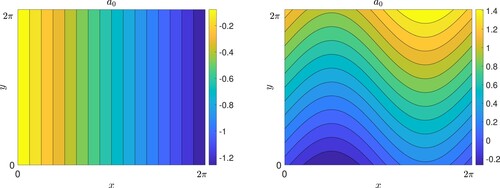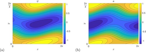We therefore adopt the following steady solution of the equations as our basic state, (17) ${\mathit{u}}_0=(U_0,\sin x),{\mathit{b}}_0=(0,B_0),\mathit{f}=(0,\mathrm{\nu sin}x+U_0\cos x),$(17) or in our scalar-based formulation (18) ${\psi }_0=U_{0}y+\cos x,{\omega }_0=\cos x,a_0=-B_{0}x,j_0=0,g=\mathrm{\nu cos}x-U_0\sin x.$(18) The basic state magnetic field is shown in figure 1(a). The stability problem is parameterised by the four quantities $\{\nu ,B_0,P,U_0\}$. Note that while the mean horizontal flow specified by the parameter $U_0$ could be removed by a Galilean transformation, the Kolmogorov flow would then become a travelling wave as the forcing does not travel with the flow $U_0$. Thus, given we take a steady Kolmogorov flow in the form (17(17) ${\mathit{u}}_0=(U_0,\sin x),{\mathit{b}}_0=(0,B_0),\mathit{f}=(0,\mathrm{\nu sin}x+U_0\cos x),$(17) ), the effect of $U_0$ cannot be eliminated by this means.

Figure 1. The magnetic field basic state for (a) vertical field (in sections 2, 3), (b) horizontal field (in sections 4, 5), with $B_0=0.7$, $\eta =0.5$. In each case field lines are depicted as contours of the corresponding magnetic potential $a_0$, with ${\mathit{b}}_0=({\mathrm{\partial }}_y{a}_0,-{\mathrm{\partial }}_x{a}_0)$ (Colour online).

To study the stability of this basic state we linearise, replacing (19) $\begin{array}{rl}\psi & ={\psi }_0+{\psi }_1+\cdots ,\omega ={\omega }_0+{\omega }_1+\cdots ,\\ a& =a_0+a_1+\cdots ,j=j_0+j_1+\cdots ,\end{array}$(19) and, droppping the subscript 1, we deduce the linear system (20) $\begin{array}{rl}& {\mathrm{\partial }}_t\omega +U_0{\mathrm{\partial }}_x\omega +\sin x({\mathrm{\partial }}_y\omega -{\mathrm{\partial }}_y\psi )=B_0{\mathrm{\partial }}_{y}j+\nu {\mathrm{\nabla }}^2\omega ,\end{array}$(20) (21) $\begin{array}{rl}& {\mathrm{\partial }}_{t}a+U_0{\mathrm{\partial }}_{x}a+\sin x{\mathrm{\partial }}_{y}a=B_0{\mathrm{\partial }}_y\psi +\eta {\mathrm{\nabla }}^{2}a,\end{array}$(21) (22) $\begin{array}{rl}& \omega =-{\mathrm{\nabla }}^2\psi ,j=-{\mathrm{\nabla }}^{2}a.\end{array}$(22) We now expand the fields in Fourier modes in x as (23) $(\psi ,\omega ,a,j)=e^{\mathrm{pt}+\mathrm{i}\mathrm{\ell x}+\mathrm{i}\mathrm{ky}}\sum _n({\Psi }_n,{\Omega }_n,A_n,J_n)e^{\mathrm{i}\mathrm{nx}}+\mathrm{c}.\mathrm{c}.,$(23) where $\mathrm{c}.\mathrm{c}.$ denotes the complex conjugate of the preceding expression. Here p is the complex growth rate of the mode, k is the wavenumber in the y-direction with k>0 without loss of generality, and ℓ is a Bloch or Floquet wavenumber in the x-direction satisfying $-1/2<\ell \le 1/2$.

Substituting these series into the linear equations (20(20) $\begin{array}{rl}& {\mathrm{\partial }}_t\omega +U_0{\mathrm{\partial }}_x\omega +\sin x({\mathrm{\partial }}_y\omega -{\mathrm{\partial }}_y\psi )=B_0{\mathrm{\partial }}_{y}j+\nu {\mathrm{\nabla }}^2\omega ,\end{array}$(20) )–(22(22) $\begin{array}{rl}& \omega =-{\mathrm{\nabla }}^2\psi ,j=-{\mathrm{\nabla }}^{2}a.\end{array}$(22) ) results in an infinite system of equations. For $\ell =0$ these may be written in the form: (24) $\begin{array}{rl}p{\Omega }_n& =-[\nu (n^2+k^2)+\mathrm{i}n{U}_0]{\Omega }_n+\frac{k}{2}(\frac{1}{(n-1{)}^2+k^2}-1){\Omega }_{n-1}\\ & -\frac{k}{2}(\frac{1}{(n+1{)}^2+k^2}-1){\Omega }_{n+1}+\mathrm{i}k{B}_0(n^2+k^2)A_n,\end{array}$(24) (25) $\begin{array}{rl}p{A}_n& =-[\eta (n^2+k^2)+\mathrm{i}n{U}_0]A_n-\frac{k}{2}{A}_{n-1}+\frac{k}{2}{A}_{n+1}+\frac{\mathrm{i}k{B}_0}{n^2+k^2}{\Omega }_n,\end{array}$(25) and for $\ell \ne 0$ we simply replace $n\to n+\ell$ wherever it appears (except as a subscript). This provides an eigenvalue problem. We take p to be the leading eigenvalue (or one of a complex conjugate pair), that is the eigenvalue having the maximum real part, and we write it with a dependence $p(k,\ell ,\nu ,B_0,P,U_0)$ in general. The real part of the growth rate, $\mathrm{Re}\{p\}$, is unchanged on the replacement $(k,\ell )\to (-k,-\ell )$.

For a numerical solution we restrict $-N\le n\le N$ for some integer N (typical values are 8, 16, 32) and solve a discrete matrix problem written in the pentadiagonal form (26) $p\left(\begin{array}{c}⋮\\ {\Omega }_n\\ A_n\\ ⋮\end{array}\right)=\left(\begin{array}{cccccccc}\ddots & \ddots & \ddots & \ddots & \ddots & \ddots & \ddots & \ddots \\ \ddots & \otimes & 0& \otimes & \otimes & \otimes & 0& \ddots \\ \ddots & 0& \otimes & \otimes & \otimes & 0& \otimes & \ddots \\ \ddots & \ddots & \ddots & \ddots & \ddots & \ddots & \ddots & \ddots \end{array}\right)\left(\begin{array}{c}⋮\\ {\Omega }_n\\ A_n\\ ⋮\end{array}\right),$(26) where ⊗ denotes the only non-zero entries. At a specified truncation N the $(4N+2)\times (4N+2)$ matrix is set up in Matlab, and an eigenvalue p with maximum real part is calculated. For a given parameter set $\{\nu ,B_0,P,U_0\}$ the maximum real growth rate is defined as (27) $\mathrm{Re}\{p_{max}(\nu ,B_0,P,U_0)\}=\underset{k,\ell }{max}\mathrm{Re}\{p(k,\ell ,\nu ,B_0,P,U_0)\},$(27) with the maximum taken over a grid of k and ℓ values.

In what follows we will start by taking $U_0=0$, $\ell =0$ and only vary the vertical wavenumber k. The maximisation is then taken over a finite range of k-values, typically 100 values in the range $0\le k\le 1$, and any complex eigenvalues appear in complex conjugate pairs. We let $k_{max}(\nu ,B_0,P)$ be the corresponding maximising wave number, and we attach the appropriate (zero or positive) imaginary part to give $p_{max}(\nu ,B_0,P)$ as the (maximum) complex instability growth rate. In summarising the instabilities of the system it is often useful to produce colour plots of $\mathrm{Re}\{p_{max}\}$ as a function in the $(\nu ,B_0)$ parameter plane for a given P; we will display many of these below, supplemented by plots of $\mathrm{Im}\{p_{max}\}$ and $k_{max}$ when these provide further useful information.

3. Numerical and analytical results: vertical field

We use the numerical code as described above to produce eigenvalues so that we can explore the dependence on parameters. Our starting point is to investigate the effect of increasing the vertical magnetic field strength $B_0$ on the classic hydrodynamic instability of Kolmogorov flow. We take the mean flow $U_0=0$ in sections 3.1, 3.2, and explore its effect in section 3.3.

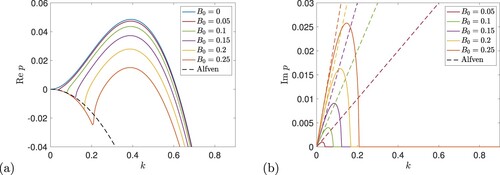
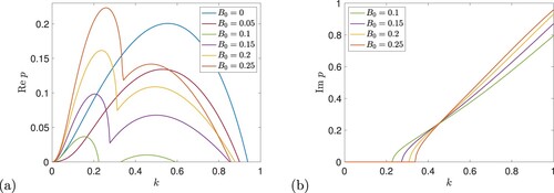
3.1. Weak vertical field branch, $U_0=0$

Figure 2(a) shows the real part of the growth rate $p(k,\nu ,B_0,P)$ for $\nu =\eta =0.4$ and so P = 1, plotted against k for given values of the magnetic field strength $B_0$. Here $B_0$ is increased from zero in steps of 0.05 as we read down the family of curves. The top curve relates to the purely hydrodynamic case. As we increase $B_0$ we note two effects: first the peak is reduced, in other words the magnetic field acts to suppress the instability, as found by Fraser et al. (2022). Secondly, for large scales, namely small k, a new branch of decaying modes appears, with growth rates largely independent of field strength. Figure 2(b) shows the imaginary part of the growth rate p. This is zero for the purely hydrodynamic case and remains zero for this branch as it is suppressed by the field. The new stable branch for low k has a non-zero imaginary part which becomes more prominent as $B_0$ is increased and we read up the curves in panel (b). Some investigation shows that the new branch is in fact a damped Alfvén wave on the vertical magnetic field. For zero background flow ${\mathit{u}}_0$, a vertical field supports Alfvén waves with (28) $p=\pm \mathrm{i}k\sqrt{B_0^2-\frac{1}{4}(\nu -\eta {)}^2{k}^2}-\frac{1}{2}(\nu +\eta )k^2,$(28) and the real and imaginary parts of this expression are shown dashed in figure 2. The real part in panel (a) is the same for all field strengths and is black dashed; in panel (b) there is a dashed straight line for each $B_0>0$, coloured appropriately, and tangent at the origin to the solid curve for that field stength. Since the Alfvén waves are modified by the background Kolmogorov flow, the agreement between solid and dashed curves in panel (a) is not perfect, but this is clearly the origin of these small-k damped modes.

Figure 2. Instability growth rate p for vertical magnetic field as a function of wave number k (with $U_0$, $\ell =0$) for $\nu =\eta =0.4$ (P = 1), and $B_0=0$ (blue), $B_0=0.05$ (red), $B_0=0.10$ (green), $B_0=0.15$ (purple), $B_0=0.20$ (orange) and $B_0=0.25$ (dark orange). Panels (a) and (b) show $\mathrm{Re}\{p\}$ and $\mathrm{Im}\{p\}$, respectively, and dashed curves show the Alfvén wave branch in (28(28) $p=\pm \mathrm{i}k\sqrt{B_0^2-\frac{1}{4}(\nu -\eta {)}^2{k}^2}-\frac{1}{2}(\nu +\eta )k^2,$(28) ) (Colour online).

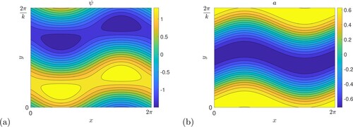
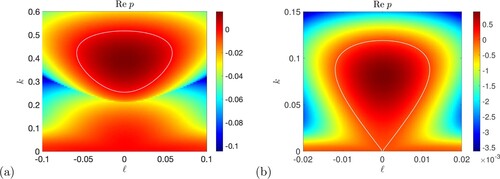
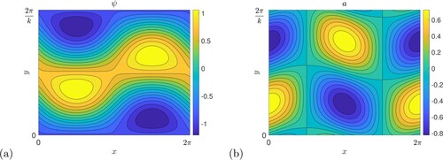
A typical unstable mode is shown in figure 3 for parameter values corresponding to the peak k = 0.4 in the lowest curve in figure 2(a), that is for the strongest field $B_0=0.25$ used. We observe the perturbation streamfunction ψ in panel (a) showing clear zonostrophic jets, and corresponding changes to the magnetic potential in panel (b); Fraser et al. (2022) refer to these as sinuous Kelvin–Helmholtz modes. Since the instabilities we observe here are obtained from the hydrodynamic problem as we increase $B_0$ from small values, we refer to this as the weak vertical field branch, to be contrasted with a strong field branch we encounter shortly.

Figure 3. Structure of a typical unstable mode, with $B_0=0.25$, $\nu =\eta =0.4$, k = 0.4; (a) shows the stream function ψ and (b) the magnetic potential a.

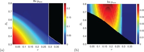
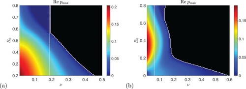
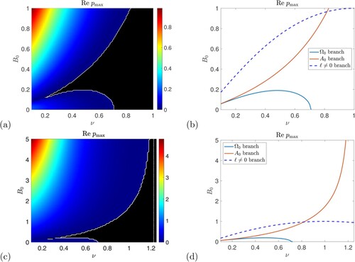
Having seen a particular example of how the magnetic field suppresses the hydrodynamic instability by plotting $p(k,\nu ,B_0,P)$, we now show results where we maximise over k for each set of the parameters. Figure 4(a) shows numerical results for $\mathrm{Re}\{p_{max}(\nu ,B_0,P)\}$ with P = 1 as a colour plot across the $(\nu ,B_0)$-plane. The white curve shows the threshold for instability, $\mathrm{Re}\{p_{max}\}=0$; the colour scale shows black for stability and then blue to yellow and red for instability and increasing growth rates. The horizontal axis $B_0=0$ is the hydrodynamic case, where the white curve crosses at ${\nu }_c=1/\sqrt{2}$. Instability occurs in the region below the white curve, and we can see that it is suppressed as $B_0$ increases, up to the point where $B_0\simeq 0.7$ and the instability is entirely eliminated. We do not show $\mathrm{Im}\{p_{max}\}$, which is zero within the region of instability.

Figure 4. Instability growth rate $\mathrm{Re}\{p_{max}\}$ for vertical field plotted in the $(\nu ,B_0)$ plane for P = 1, $\ell =0$, $U_0=0$, $0.01\le \nu \le 0.8$. Panel (a) shows the numerical computation of growth rates with the threshold $\mathrm{Re}\{p_{max}\}=0$ given by a white curve, and panel (b) the analytical maximum growth rate from (30(30) $p_{max}(\nu ,B_0,P)=-\frac{\sqrt{2}P}{1+P^2}{B}_0^2+\frac{\sqrt{2}}{3}(\frac{1}{\sqrt{2}}-\nu {)}^2,k_{max}^2=\frac{\sqrt{2}}{3}(\frac{1}{\sqrt{2}}-\nu ).$(30) ) and threshold from (31(31) $B_0(\nu ,P)=\sqrt{\frac{1+P^2}{3P}}(\frac{1}{\sqrt{2}}-\nu ).$(31) ). Black shows zero growth rates.

Note that in the limit $k\to 0$ all modes tend to neutral stability, $p(k)\to 0$; thus always $\mathrm{Re}\{p_{max}\}\ge 0$ because of the maximisation over k and we can never obtain a negative maximum growth rate. Thus, strictly speaking setting $\mathrm{Re}\{p_{max}\}=0$ gives not a curve but a two-dimensional region of the parameter space, that is both the white curve and the solid black region in figure 4(a). For simplicity, here and onwards, when we refer to the threshold white curve $\mathrm{Re}\{p_{max}\}=0$ we in fact mean the curve separating regions of stability where $\mathrm{Re}\{p_{max}\}=0$ from regions of instability $\mathrm{Re}\{p_{max}\}>0$. Since numerically we maximise over a discrete set of k values with $0<k\le 1$, a stable parameter set is flagged by a numerical measurement of $\mathrm{Re}\{p_{max}\}$ being small and negative rather than exactly zero. This makes the numerical white contour easy to produce, and then negative values are mapped onto black on the colour scale, to show stability.

We can develop perturbation theory (as in, for example, Frisch et al. 1996, Manfroi and Young 2002) to calculate approximate growth rates valid for $k\to 0$. In Appendix C we give the details. One key result is the formula (C.20(C.20) $p=-\frac{\sqrt{2}P}{1+P^2}{B}_0^2+2(\frac{1}{\sqrt{2}}-\nu )k^2-\frac{3}{\sqrt{2}}{k}^4+\cdots .$(C.20) ), (29) $p(k,\nu ,B_0,P)=-\frac{\sqrt{2}P}{1+P^2}{B}_0^2+2(\frac{1}{\sqrt{2}}-\nu )k^2-\frac{3}{\sqrt{2}}{k}^4+\cdots ,$(29) giving the growth rate, and showing clearly how the effect of the magnetic field is to suppress the hydrodynamic $B_0=0$ instability (as seen in figure 2(a)). For unstable modes it is necessary that $\nu <1/\sqrt{2}$ and in this case maximising the growth rate over values of k gives (30) $p_{max}(\nu ,B_0,P)=-\frac{\sqrt{2}P}{1+P^2}{B}_0^2+\frac{\sqrt{2}}{3}(\frac{1}{\sqrt{2}}-\nu {)}^2,k_{max}^2=\frac{\sqrt{2}}{3}(\frac{1}{\sqrt{2}}-\nu ).$(30) Putting $p_{max}=0$ gives the threshold of instability as the straight line in the $(\nu ,B_0)$-plane: (31) $B_0(\nu ,P)=\sqrt{\frac{1+P^2}{3P}}(\frac{1}{\sqrt{2}}-\nu ).$(31) Figure 4(b) shows the theoretical growth rate and the threshold marked by a white (straight) line, showing good agreement with the full numerics. The perturbation theory is developed about the point ${\nu }_c=1/\sqrt{2}$, $B_0=0$ of the onset of the hydrodynamic instability. Hence the agreement is particularly good near this point; elsewhere the theory gives results that can be seen from the figure to be qualitatively correct only.

The scalings chosen in the theory in Appendix C are aimed at tracking the effect of magnetic field in suppressing Kolmogorov flow instabilities, which pull the $B_0=0$ peak in figure 2(a) downwards as $B_0$ is increased. The scalings used do not relate to the emerging, stable Alfvén wave branch seen for low k, approximated roughly by (28(28) $p=\pm \mathrm{i}k\sqrt{B_0^2-\frac{1}{4}(\nu -\eta {)}^2{k}^2}-\frac{1}{2}(\nu +\eta )k^2,$(28) ) (dashed). It is worth noting that while the $B_0=0$ purely hydrodynamic instability is flagged by a sign change of the effective viscosity ${\nu }_E$ at $\nu ={\nu }_c$ and so is of negative effective viscosity type (Dubrulle and Frisch 1991), this is not the case once $B_0>0$. As may be seen from figure 2(a), for any fixed $B_0>0$, in the limit $k\to 0$ we have $p\sim -{\nu }_E{k}^2$ with ${\nu }_E=\frac{1}{2}(\nu +\eta )>0$ from (28(28) $p=\pm \mathrm{i}k\sqrt{B_0^2-\frac{1}{4}(\nu -\eta {)}^2{k}^2}-\frac{1}{2}(\nu +\eta )k^2,$(28) ). In other words for any $B_0>0$ the instability ceases to be a negative effective viscosity instability, which explains why our analysis for $k\to 0$ cannot precisely track the numerical white curve in figure 4(a), except near the point $\nu ={\nu }_c$, $B_0=0$.

The theoretical value of $B_0$ which suppresses instability on the weak field branch for all ν is given by taking $\nu =0$ in (31(31) $B_0(\nu ,P)=\sqrt{\frac{1+P^2}{3P}}(\frac{1}{\sqrt{2}}-\nu ).$(31) ), (32) $B_0\simeq B_{\ast }=\sqrt{\frac{1+P^2}{6P}},$(32) with $B_{\ast }\simeq 0.58$ for P = 1 in panel (b), which is a little lower than the actual value $B_{\ast }\simeq 0.7$ seen for the numerical results in panel (a). However exploring numerically for a range of Prandtl numbers $0.1\le P\le 10$, we find that this extrapolated threshold generally shows poor agreement with the numerical threshold, which remains around $B_{\ast }\simeq 0.7$ over this range. This was also observed by Fraser et al. (2022), who calculated $B_{\ast }^2\simeq 0.5$ for the instability threshold of the vertical field and Kolmogorov flow configuration in ideal MHD, $\eta =\nu =0$.

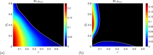
3.2. Strong vertical field branch, $U_0=0$

Although the magnetic field acts to suppress the instability for magnetic Prandtl number P = 1, this is not the whole picture, and investigations for P<1 show the presence of a strong vertical field branch, as found by Fraser et al. (2022). Figure 5 shows (a) the real part and (b) imaginary part of the growth $p_{max}(\nu ,B_0,P)$ for $P=1/2$, that is $\eta =2\nu$. The threshold $\mathrm{Re}\{p_{max}\}=0$ is shown as a white curve in panel (a). Looking from the bottom of figure 5(a) (increasing $B_0$) we see that the curving white line, showing the weak field branch in figure 4(a), turns to become a near-vertical line, demarcating a new branch with non-zero frequency $\mathrm{Im}\{p_{max}\}$ evident in figure 5(b).

Figure 5. Shown are numerical calculations of (a) the instability growth rate $\mathrm{Re}\{p_{max}\}$ and (b) the frequency $\mathrm{Im}\{p_{max}\}$ for vertical field plotted in the $(\nu ,B_0)$ plane, with $P=1/2$, $0.01\le \nu \le 0.4$. Black shows zero values and the solid white curve in panel (a) shows the numerical threshold $\mathrm{Re}\{p_{max}\}=0$ for instability; the dotted white line in (a) shows the theoretical threshold ${\nu }_{\ast }$ from (35(35) $\nu <{\nu }_{\ast }=\sqrt{\frac{P}{2}\frac{1-P}{1+P}}\mathrm{or}R>R_{\ast }=\sqrt{\frac{2}{P}\frac{1+P}{1-P}}.$(35) ) (Colour online).

This strong vertical field branch is analysed in Appendix B, using a scaling in which $B_0=\mathrm{O}(k^{-1})$ as $k\to 0$ (and allowing a mean flow $U_0\ne 0$). The pertubation theory then involves a leading order undamped Alfvén wave with frequency $p_0=\mathrm{i}k{B}_0=\mathrm{O}(1)$, in other words the wave whose frequency and decay rate are given in (28(28) $p=\pm \mathrm{i}k\sqrt{B_0^2-\frac{1}{4}(\nu -\eta {)}^2{k}^2}-\frac{1}{2}(\nu +\eta )k^2,$(28) ) in the absence of any background fluid flow. The coupling of this wave with the Kolmogorov flow field leads to potential instability with a growth rate given in (B.15(B.15) $\mathrm{Re}\{p\}=\frac{\frac{1}{4}\mathrm{\nu \eta }(\eta -\nu )k^2}{{\nu }^2{\eta }^2+k^2{B}_0^2(\nu +\eta {)}^2}-\frac{1}{2}(\nu +\eta )k^2+\cdots .$(B.15) ) for $U_0=0$ as (33) $\mathrm{Re}\{p\}=\frac{\frac{1}{4}\mathrm{\nu \eta }(\eta -\nu )k^2}{{\nu }^2{\eta }^2+k^2{B}_0^2(\nu +\eta {)}^2}-\frac{1}{2}(\nu +\eta )k^2+\cdots .$(33) An equivalent expression is found in Fraser et al. (2022) by approximating a quartic dispersion relation. Evidently we need $\eta >\nu$ for instability, in other words P<1; the instability of the large-scale Alfvén wave appears to take a double-diffusive form. We can also write a power series expansion $p=-{\nu }_E{k}^2+\dots$ and identify¹ (34) $-{\nu }_E=\frac{1}{4}{\nu }^{-1}{\eta }^{-1}(\eta -\nu )-\frac{1}{2}(\nu +\eta ).$(34) This in fact simply corresponds to setting $k{B}_0=0$ in (33(33) $\mathrm{Re}\{p\}=\frac{\frac{1}{4}\mathrm{\nu \eta }(\eta -\nu )k^2}{{\nu }^2{\eta }^2+k^2{B}_0^2(\nu +\eta {)}^2}-\frac{1}{2}(\nu +\eta )k^2+\cdots .$(33) ) above. As explained by Fraser et al. (2022), the fact that ${\nu }_E$ changes sign flags the instability as of negative effective viscosity type and rearranging ${\nu }_E<0$ gives the stability threshold (35) $\nu <{\nu }_{\ast }=\sqrt{\frac{P}{2}\frac{1-P}{1+P}}\mathrm{or}R>R_{\ast }=\sqrt{\frac{2}{P}\frac{1+P}{1-P}}.$(35) For example if $P=1/2$ then ${\nu }_{\ast }=1/\sqrt{12}\simeq 0.28$, shown dotted in figure 5(a), in good agreement with the numerical vertical solid white line. Thus the instability persists for arbitrarily large magnetic fields, provided the viscosity is below this Prandtl-number dependent threshold, in other words provided the Reynolds number $R>R_{\ast }$.

All the above results have been taken for Bloch wave number $\ell =0$. Introducing ℓ brings in an extra degree of freedom and allows the possibility of new instabilities. However in the vertical field case with $U_0=0$, increasing $|\ell |$ from zero appears to have only a stabilising effect (Fraser et al. 2022). For example figure 6 shows growth rates in the $(\ell ,k)$-plane for weak and strong field cases in panels (a) and (b). The white curves give the threshold $\mathrm{Re}\{p\}=0$: inside these curves growth rates are positive. In each case we see that the instability present on the vertical axis $\ell =0$, for a range of k, extends into islands of unstable modes including non-zero values of ℓ. However to either side of the vertical axis, the growth rates are diminished and so allowing $\ell \ne 0$ has little impact. For this reason we will not consider ℓ further for the vertical field case, except to mention that the theory in Appendix B may be extended to incorporate $\ell \ne 0$, as detailed in Algatheem (2023).

Figure 6. Instability growth rate $\mathrm{Re}\{p\}$ for vertical field as a function of $(\ell ,k)$ for (a) $\nu =\eta =0.4$ (P = 1) with $B_0=0.25$, and (b) $\nu =0.2$, $\eta =0.4$ (P = 0.5) with $B_0=0.7$. The white contour lines give $\mathrm{Re}\{p\}=0$; inside growth rates are positive (Colour online).

3.3. Instabilities for $U_0\ne 0$

We now consider the effect of a mean flow $U_0\ne 0$ on the instabilities in the vertical field case, with all four parameters involved, that is $\{\nu ,P,B_0,U_0\}$. To navigate all the possible numerical results we could present, it is helpful to start from the asymptotic theory and then select parameter sets to both confirm the results and also to reveal further information. Note that we have to limit our explorations in view of the dimensionality of the parameter space and that our focus is on the theoretical predictions. We take $U_0\ge 0$ without loss of generality in our discussion and take $\ell =0$ in this section.

The theory for the weak field branch in Appendix C is based around the point of onset $({\nu }_c,B_0=0)$ of the purely hydrodynamic instability, with ${\nu }_c=1/\sqrt{2}$ for $U_0=0$. For $U_0\ne 0$ this hydrodynamic threshold is reduced to (36) ${\nu }_c(U_0)=\sqrt{\frac{1}{2}-U_0^2},\mathrm{for}{U}_0<1/\sqrt{2},B_0=0,$(36) with no instability at all if $U_0\ge 1/\sqrt{2}$. Including a weak magnetic field $B_0>0$ gives the equation for the threshold, accurate in the vicinity of the point of onset $({\nu }_c,B_0=0)$ as (37) $B_0(\nu ,P,U_0)=\sqrt{\frac{1+\frac{1}{2}\delta }{P(1+4{\nu }_c^2)}}2{\nu }_c^2({\nu }_c-\nu ),\delta \equiv \frac{P^2}{{\nu }_c^2(1-P^2)+\frac{1}{2}{P}^2},$(37) analogous to (31(31) $B_0(\nu ,P)=\sqrt{\frac{1+P^2}{3P}}(\frac{1}{\sqrt{2}}-\nu ).$(31) ).

The theory for the strong field branch in Appendix B also includes $U_0$ in the most general case. The equation for the growth rate $\mathrm{Re}\{p\}$ (analogous to (33(33) $\mathrm{Re}\{p\}=\frac{\frac{1}{4}\mathrm{\nu \eta }(\eta -\nu )k^2}{{\nu }^2{\eta }^2+k^2{B}_0^2(\nu +\eta {)}^2}-\frac{1}{2}(\nu +\eta )k^2+\cdots .$(33) ) for $U_0=0$) is messy and unilluminating for $U_0\ne 0$; we give p in (B.16(B.16) $p=\frac{1}{4}\Delta (\eta -\nu )[\mathrm{\nu \eta }+\mathrm{i}k{B}_0(\nu +\eta )-U_0^2]k^2-\frac{1}{2}(\nu +\eta )k^2+\cdots ,$(B.16) ), (B.17(B.17) ${\Delta }^{-1}={\nu }^2{\eta }^2+U_0^2({\nu }^2+{\eta }^2-4k^2{B}_0^2)-k^2{B}_0^2(\nu +\eta {)}^2+2\mathrm{i}k{B}_0(\nu +\eta )(\mathrm{\nu \eta }+U_0^2)+U_0^4.$(B.17) ). However just as we obtained (34(34) $-{\nu }_E=\frac{1}{4}{\nu }^{-1}{\eta }^{-1}(\eta -\nu )-\frac{1}{2}(\nu +\eta ).$(34) ) from (33(33) $\mathrm{Re}\{p\}=\frac{\frac{1}{4}\mathrm{\nu \eta }(\eta -\nu )k^2}{{\nu }^2{\eta }^2+k^2{B}_0^2(\nu +\eta {)}^2}-\frac{1}{2}(\nu +\eta )k^2+\cdots .$(33) ) by setting $k{B}_0=0$ to extract the coefficient $-{\nu }_E$ of $k^2$ in the growth rate p, here we can do the same to obtain (38) $-{\nu }_E=\frac{\frac{1}{4}(\eta -\nu )(\mathrm{\nu \eta }-U_0^2)}{({\nu }^2+U_0^2)({\eta }^2+U_0^2)}-\frac{1}{2}(\nu +\eta ),$(38) from (B.16(B.16) $p=\frac{1}{4}\Delta (\eta -\nu )[\mathrm{\nu \eta }+\mathrm{i}k{B}_0(\nu +\eta )-U_0^2]k^2-\frac{1}{2}(\nu +\eta )k^2+\cdots ,$(B.16) ), (B.17(B.17) ${\Delta }^{-1}={\nu }^2{\eta }^2+U_0^2({\nu }^2+{\eta }^2-4k^2{B}_0^2)-k^2{B}_0^2(\nu +\eta {)}^2+2\mathrm{i}k{B}_0(\nu +\eta )(\mathrm{\nu \eta }+U_0^2)+U_0^4.$(B.17) ). Looking for where ${\nu }_E$ changes sign gives a quadratic equation in ${\nu }_{\ast }^2$ which may be written as (39) $\frac{P}{2}\frac{1-P}{1+P}({\nu }_{\ast }^2-P{U}_0^2)=({\nu }_{\ast }^2+U_0^2)({\nu }_{\ast }^2+P^2{U}_0^2).$(39) Although this can then be solved to give an explicit formula for ${\nu }_{\ast }$, we do not do so here as it is unwieldy; for $U_0=0$, (39(39) $\frac{P}{2}\frac{1-P}{1+P}({\nu }_{\ast }^2-P{U}_0^2)=({\nu }_{\ast }^2+U_0^2)({\nu }_{\ast }^2+P^2{U}_0^2).$(39) ) results in the expression displayed in (35(35) $\nu <{\nu }_{\ast }=\sqrt{\frac{P}{2}\frac{1-P}{1+P}}\mathrm{or}R>R_{\ast }=\sqrt{\frac{2}{P}\frac{1+P}{1-P}}.$(35) ). Equation (39(39) $\frac{P}{2}\frac{1-P}{1+P}({\nu }_{\ast }^2-P{U}_0^2)=({\nu }_{\ast }^2+U_0^2)({\nu }_{\ast }^2+P^2{U}_0^2).$(39) ) is then key to our study of the strong field branch for $U_0\ne 0$. If we vary ν holding P and $U_0$ constant, whenever ν crosses a root ${\nu }_{\ast }$ of the equation then ${\nu }_E$ changes sign and we are at the threshold of a negative effective viscosity instability. We will therefore display the real, positive roots ${\nu }_{\ast }$ of (39(39) $\frac{P}{2}\frac{1-P}{1+P}({\nu }_{\ast }^2-P{U}_0^2)=({\nu }_{\ast }^2+U_0^2)({\nu }_{\ast }^2+P^2{U}_0^2).$(39) ) as functions of the parameters $\{P,U_0\}$.

We consider first 0<P<1. Figure 7(a) shows real positive roots ${\nu }_{\ast }$ of (39(39) $\frac{P}{2}\frac{1-P}{1+P}({\nu }_{\ast }^2-P{U}_0^2)=({\nu }_{\ast }^2+U_0^2)({\nu }_{\ast }^2+P^2{U}_0^2).$(39) ) as functions of P for given values of $U_0$. For $U_0=0$ (blue curve) the roots are ${\nu }_{\ast }=0$ and the curve showing ${\nu }_{\ast }$ given in (35(35) $\nu <{\nu }_{\ast }=\sqrt{\frac{P}{2}\frac{1-P}{1+P}}\mathrm{or}R>R_{\ast }=\sqrt{\frac{2}{P}\frac{1+P}{1-P}}.$(35) ). Between this curve and the horizontal axis is an island inside which ${\nu }_E<0$ and instability is present. As $U_0$ is increased, we obtain a nested, contracting family of islands: for any points $(\nu ,P)$ inside the island for that value of $U_0$ there is a negative ${\nu }_E$ instability. From figure 7(a) it is then evident that as $U_0$ is increased from zero, the range of values of P supporting instability shrinks down to $0<P_{\ast 1}(U_0)<P<P_{\ast 2}(U_0)<1$. At the same time the range of viscosities for instability also decreases and becomes bounded away from zero, taking the form $0<{\nu }_{\ast 1}(P,U_0)<\nu <{\nu }_{\ast 2}(P,U_0)$, bounded by two real roots of (39(39) $\frac{P}{2}\frac{1-P}{1+P}({\nu }_{\ast }^2-P{U}_0^2)=({\nu }_{\ast }^2+U_0^2)({\nu }_{\ast }^2+P^2{U}_0^2).$(39) ).

Figure 7. Real positive roots ${\nu }_{\ast }$ of (39(39) $\frac{P}{2}\frac{1-P}{1+P}({\nu }_{\ast }^2-P{U}_0^2)=({\nu }_{\ast }^2+U_0^2)({\nu }_{\ast }^2+P^2{U}_0^2).$(39) ) plotted against P for (a) $0\le P\le 1$ and $U_0=0$ (blue), $U_0=0.04$ (red), $U_0=0.08$ (green), $U_0=0.12$ (purple) and $U_0=0.16$ (orange), and (b) $1\le P\le 5$ and $U_0=0.1$ (blue), $U_0=0.2$ (red), $U_0=0.3$ (green), $U_0=0.4$ (purple) and $U_0=0.5$ (orange). The vertical dashed line is at (a) P = 0.5 and (b) P = 2 (Colour online).

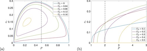
To take a specific example, for say $U_0=0.12$, the purple curve in figure 7(a), there are real roots for ${\nu }_{\ast }$ only in the approximate range $0.05\simeq P_{\ast 1}(U_0)<P<P_{\ast 2}(U_0)\simeq 0.61$, and it is only in this range of P that the strong field branch can show negative effective viscosity instability for this value of $U_0$. Focusing now on say P = 0.5 (vertical dashed line), the instability occurs for $0.11\simeq {\nu }_{\ast 1}(P,U_0)<\nu <{\nu }_{\ast 2}(P,U_0)\simeq 0.23$.

As $U_0$ is increased further the islands of negative ${\nu }_E$ shrink in the $(P,\nu )$ plane in figure 7(a), until at the value $U_0\simeq 0.164$ the range of P shrinks to $P_{\ast 1}=P_{\ast 2}\simeq 0.23$ and the range of ν to ${\nu }_{\ast 1}={\nu }_{\ast 2}\simeq 0.15$. At this point the mean flow $U_0$ has entirely stabilised the P<1 negative effective viscosity instability for strong vertical field.

To test these results for 0<P<1 and $U_0>0$ numerically, we take P = 0.5 and in figure 8(a) we show growth rates in the $(\nu ,B_0)$ plane for $U_0=0.12$. Here as discussed above, theory gives a negative effective viscosity instability for $0.11\simeq {\nu }_{\ast 1}<\nu <{\nu }_{\ast 2}\simeq 0.23$ and these bounds are marked on the panel by dotted vertical lines. There is instability present across this range of ν values, and in fact ${\nu }_{2\ast }$ gives good agreement with the upper limit (in terms of ν) of the strong field branch in figure 8(a). What about the lower limit, ${\nu }_{\ast 1}\simeq 0.11$? This value gives the lower limit for negative effective viscosity instabilities signalled by ${\nu }_E<0$, and for ν below ${\nu }_{\ast 1}$ theory predicts that ${\nu }_E>0$. However there can be further instabilities present corresponding to larger values of k and not $k\to 0$, as seen and discussed earlier for the weak field branch in figure 2. In short, the condition ${\nu }_E<0$ is sufficient for instability, of negative effective viscosity type, but not necessary for instability as other types may be present. Further investigation (which we will not detail here) for $\nu <{\nu }_{\ast 1}\simeq 0.11$ confirms that ${\nu }_E>0$ and $\mathrm{Re}\{p(k)\}$ is negative when $k\to 0$ as indicated by theory, but the curve $\mathrm{Re}\{p(k)\}$ then rises for increasing k, and instabilities are present for $k=\mathrm{O}(1)$.

Figure 8. Numerical computations of the instability growth rate $\mathrm{Re}\{p_{max}\}$ for vertical field plotted in the $(\nu ,B_0)$ plane for P = 0.5, $\ell =0$, $0.01\le \nu \le 0.5$ with (a) $U_0=0.12$ and (b) $U_0=0.2$. Black shows zero values and the solid white curve shows the numerical threshold $\mathrm{Re}\{p_{max}\}=0$ for instability; the dotted white lines in panel (a) show the theoretical thresholds ${\nu }_{\ast }$ from (39(39) $\frac{P}{2}\frac{1-P}{1+P}({\nu }_{\ast }^2-P{U}_0^2)=({\nu }_{\ast }^2+U_0^2)({\nu }_{\ast }^2+P^2{U}_0^2).$(39) ) (Colour online).

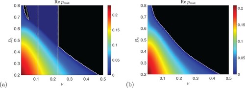
Figure 8(b) shows growth rates for P = 0.5 again but now $U_0=0.2$, when from figure 7(a) there are no values of ν giving negative effective viscosity instability. In the figure there are no vertical lines from theory or numerics. Instabilities remain, hugging the vertical axis, but investigation of $p(k)$ (which we do not detail here) shows that these are not associated with negative effective viscosity: the curve $\mathrm{Re}\{p(k)\}$ shows negative values, downwards quadratic behaviour, for small k, confirming that ${\nu }_E>0$.

We now consider P>1 and return to figure 7, panel (b), which shows solutions ${\nu }_{\ast }$ to (39(39) $\frac{P}{2}\frac{1-P}{1+P}({\nu }_{\ast }^2-P{U}_0^2)=({\nu }_{\ast }^2+U_0^2)({\nu }_{\ast }^2+P^2{U}_0^2).$(39) ) plotted against P for various values of $U_0$ in the range $0<U_0<1/\sqrt{2}$. It is evident that there is a new branch of ${\nu }_E<0$ instabilities present for $P>P_{\ast }(U_0)>1$. For each value of P in this range, instabilities occur if $0<\nu <{\nu }_{\ast }(P,U_0)$. For example, in the concrete case $U_0=0.2$ (red curve) instabilities occur for pairs $(P,\nu )$ below this curve. Thus instability can occur for some viscosity provided $P>P_{\ast }(U_0)\simeq 1.17$. If we now specify P = 2 (dashed line) then instabilities are predicted to occur for $0<\nu <{\nu }_{\ast }(P,U_0)\simeq 0.19$.

To test this, figure 9 shows growth rates in the $(\nu ,B_0)$ plane for P = 2. In figure 9(a) we have $U_0=0.2$ and see a strong field branch whose numerical threshold (white curve) is given accurately by the theoretical value of ${\nu }_{\ast }\simeq 0.19$ (dashed line). Figure 9(b) shows a case of $U_0=0.4$, where the plot in figure 7(b) predicts instability below a threshold ${\nu }_{\ast }\simeq 0.061$ (dashed line). Indeed, there is instability for ν below this threshold, confirming the theory; there is also instability above the threshold, up to ν around 0.15 but dependent on field strength $B_0$. Again futher investigation of the behaviour of $\mathrm{Re}\{p(k)\}$ confirms that for $\nu <{\nu }_{\ast }\simeq 0.061$ instabilities are of negative effective viscosity type, while for $\nu >{\nu }_{\ast }$ they are not. For larger values of $U_0$ the negative ${\nu }_E$ instability switches off for P = 2; for example for U = 0.5 (orange curve) in figure 7(b) there is no unstable range of ν with P = 2. We do not present plots in the $(\nu ,B_0)$ plane for this case, as they simply begin to resemble those in figure 11(b) below.

Figure 9. Numerical computations of the instability growth rate $\mathrm{Re}\{p_{max}\}$ for vertical field plotted in the $(\nu ,B_0)$ plane for P = 2, $\ell =0$, with (a) $U_0=0.2$, $0.01\le \nu \le 0.5$ and (b) $U_0=0.4$, $0.01\le \nu \le 0.6$. Black shows zero values and the solid white curve shows the numerical threshold $\mathrm{Re}\{p_{max}\}=0$ for instability; the dotted white line in each panel shows the theoretical threshold ${\nu }_{\ast }$ from (39(39) $\frac{P}{2}\frac{1-P}{1+P}({\nu }_{\ast }^2-P{U}_0^2)=({\nu }_{\ast }^2+U_0^2)({\nu }_{\ast }^2+P^2{U}_0^2).$(39) ) (Colour online).

An example of the fields from an unstable mode in the strong field branch is shown in figure 10, for $U_0=0.2$, $B_0=0.8$, $\nu =0.1$, P = 2; see figure 7(b). It has a clear Alfvén wave character, with similar structure for the field and flow indicating motion largely transverse to the vertical field.

Figure 10. A typical unstable mode, with $U_0=0.2$, $B_0=0.8$, $\nu =0.1$, P = 2, $k=0.08$ from the strong field branch. Panel (a) shows the stream function ψ and (b) the magnetic potential a (Colour online).

Finally we look at P = 1 and $U_0>0$ when theory gives no negative effective viscosity instabilities, as seen in figure 7, or from (39(39) $\frac{P}{2}\frac{1-P}{1+P}({\nu }_{\ast }^2-P{U}_0^2)=({\nu }_{\ast }^2+U_0^2)({\nu }_{\ast }^2+P^2{U}_0^2).$(39) ). Figure 11 shows results for (a) $U_0=0.2$ and (b) 0.5. The region of instability in figure 11(a) extends vertically compared with the corresponding $U_0=0$ case in figure 4(a). With increasing $U_0$ this breaks up into two islands of instability in figure 11(b) (intermediate pictures are similar to figure 9(b) above). Notable is the pulling in of the purely hydrodynamic $B_0=0$ threshold $\nu ={\nu }_c(U_0)$ on the horizontal axis (also visible in figure 9(b)), according to (36(36) ${\nu }_c(U_0)=\sqrt{\frac{1}{2}-U_0^2},\mathrm{for}{U}_0<1/\sqrt{2},B_0=0,$(36) ), and in fact the lower island vanishes completely if $U_0>1/\sqrt{2}$ (not shown here). Formula (37(37) $B_0(\nu ,P,U_0)=\sqrt{\frac{1+\frac{1}{2}\delta }{P(1+4{\nu }_c^2)}}2{\nu }_c^2({\nu }_c-\nu ),\delta \equiv \frac{P^2}{{\nu }_c^2(1-P^2)+\frac{1}{2}{P}^2},$(37) ) has also been checked to work in the vicinity of the purely hydrodynamic threshold in these cases.

Figure 11. Numerical computations of the instability growth rate $\mathrm{Re}\{p_{max}\}$ for vertical field plotted in the $(\nu ,B_0)$ plane for P = 1, $\ell =0$, with (a) $U_0=0.2$, $0.01\le \nu \le 0.7$ and (b) $U_0=0.5$, $0.01\le \nu \le 0.6$. The numerical threshold $\mathrm{Re}\{p_{max}\}=0$ is given by a white curve and black shows zero growth rates.

4. Governing equations: horizontal field, with $U_0=0$

In this section we study the stability of Kolmogorov flow in the presence of horizontal field $B_0$, and to reduce the complexity of the problem we restrict to the case of zero horizontal mean flow, $U_0=0$. We thus adopt the following basic state, a steady solution of equations (9(9) $\begin{array}{rl}& {\mathrm{\partial }}_t\mathit{u}+\mathit{u}\cdot \mathrm{\nabla }\mathit{u}=-\mathrm{\nabla }\varpi +\mathit{j}\times \mathit{b}+\nu {\mathrm{\nabla }}^2\mathit{u}+\mathit{f},\end{array}$(9) )–(11(11) $\begin{array}{rl}& \mathrm{\nabla }\cdot \mathit{u}=0,\mathrm{\nabla }\cdot \mathit{b}=0,\mathit{j}=\mathrm{\nabla }\times \mathit{b}.\end{array}$(11) ): (40) ${\mathit{u}}_0=(0,\sin x),{\mathit{b}}_0=(B_0,{\eta }^{-1}{B}_0\cos x),\mathit{f}=(0,(\nu +{\eta }^{-1}{B}_0^2)\sin x),$(40) or in the scalar formulation, (41) $\begin{array}{rl}& {\psi }_0=\cos x,{\omega }_0=\cos x,a_0=B_0(y-{\eta }^{-1}\sin x),\\ & j_0=-{\eta }^{-1}{B}_0\sin x,g=(\nu +{\eta }^{-1}{B}_0^2)\cos x.\end{array}$(41) The basic state magnetic field is shown in figure 1(b), with horizontal field lines distorted by the background Kolmogorov flow, becoming increasingly extended in the limit of small η. Note, to pick up a comment in the introduction, that the body force required to maintain the Kolmogorov flow increases with field strength $B_0$ and with magnetic Reynolds number $R_m={\eta }^{-1}$, unlike in many large-scale simulations of zonostrophic instability, where the magnitude of a random forcing is held fixed, while other parameters are varied.

The stability problem is parameterised by $\{\nu ,B_0,P,U_0=0\}$. The corresponding linear system is (42) $\begin{array}{rl}& {\mathrm{\partial }}_t\omega +\sin x({\mathrm{\partial }}_y\omega -{\mathrm{\partial }}_y\psi )=B_0{\mathrm{\partial }}_{x}j+{\eta }^{-1}{B}_0\cos x({\mathrm{\partial }}_{y}j-{\mathrm{\partial }}_{y}a)+\nu {\mathrm{\nabla }}^2\omega ,\end{array}$(42) (43) $\begin{array}{rl}& {\mathrm{\partial }}_{t}a+\sin x{\mathrm{\partial }}_{y}a=B_0{\mathrm{\partial }}_x\psi +{\eta }^{-1}{B}_0\cos x{\mathrm{\partial }}_y\psi +\eta {\mathrm{\nabla }}^{2}a,\end{array}$(43) (44) $\begin{array}{rl}& \omega =-{\mathrm{\nabla }}^2\psi ,j=-{\mathrm{\nabla }}^{2}a,\end{array}$(44) where the fields represent the perturbation to the basic state. The resulting equations for the Fourier modes in x are (45) $\begin{array}{rl}p{\Omega }_n& =-\nu (n^2+k^2){\Omega }_n+\frac{k}{2}(\frac{1}{(n-1{)}^2+k^2}-1){\Omega }_{n-1}\\ & -\frac{k}{2}(\frac{1}{(n+1{)}^2+k^2}-1){\Omega }_{n+1}\\ & +\mathrm{i}n{B}_0(n^2+k^2)A_n+\frac{\mathrm{i}k{B}_0}{2\eta }[(n-1{)}^2+k^2-1]A_{n-1}\\ & +\frac{\mathrm{i}k{B}_0}{2\eta }[(n+1{)}^2+k^2-1]A_{n+1},\end{array}$(45) (46) $\begin{array}{rl}p{A}_n& =-\eta (n^2+k^2)A_n-\frac{k}{2}{A}_{n-1}+\frac{k}{2}{A}_{n+1}\\ & +\frac{\mathrm{i}n{B}_0}{n^2+k^2}{\Omega }_n+\frac{\mathrm{i}k{B}_0}{2\eta }\frac{1}{(n-1{)}^2+k^2}{\Omega }_{n-1}+\frac{\mathrm{i}k{B}_0}{2\eta }\frac{1}{(n+1{)}^2+k^2}{\Omega }_{n+1},\end{array}$(46) for $\ell =0$ and, as elsewhere, for $\ell \ne 0$ we replace n by $n+\ell$. This infinite system of linear equations may then be truncated and set up as a matrix eigenvalue problem, analogously to that in (26(26) $p\left(\begin{array}{c}⋮\\ {\Omega }_n\\ A_n\\ ⋮\end{array}\right)=\left(\begin{array}{cccccccc}\ddots & \ddots & \ddots & \ddots & \ddots & \ddots & \ddots & \ddots \\ \ddots & \otimes & 0& \otimes & \otimes & \otimes & 0& \ddots \\ \ddots & 0& \otimes & \otimes & \otimes & 0& \otimes & \ddots \\ \ddots & \ddots & \ddots & \ddots & \ddots & \ddots & \ddots & \ddots \end{array}\right)\left(\begin{array}{c}⋮\\ {\Omega }_n\\ A_n\\ ⋮\end{array}\right),$(26) ) for vertical field; the matrix now takes a heptadiagonal form.

5. Numerical and analytical results: horizontal field

We have used Matlab to obtain growth rates $p(k,\ell ,\nu ,B_0,P)$ (here $U_0=0$) and we focus first on the case $\ell =0$.

5.1. Instability for Bloch wave number $\ell =0$

With zero Bloch wave number ℓ, the instability has periodicity $2\pi$ in the x-direction and $2\pi /k$ in the y-direction. Figure 12 shows plots of the growth rate $p(k,\nu ,B_0,P)$ against k for $\nu =\eta =0.1$ (P = 1) and $B_0$ increasing as detailed in the caption. Focusing on the real part of p in panel (a) we observe that the magnetic field initially suppresses the instability, going from the blue $B_0=0$ curve to the lower, red $B_0=0.05$ curve. However increasing $B_0$ further, the green $B_0=0.1$ curve reveals a double-peaked growth rate and then these two peaks increase as $B_0$ is increased, as indicated in the figure caption. For these stronger fields, the second peak is the lower of the two, and is associated with non-zero imaginary part $\mathrm{Im}\{p\}$ of the growth rate, as shown in panel (b), while the dominant instability of the first peak has $\mathrm{Im}\{p\}=0$.²

Figure 12. Instability growth rate p for horizontal field as a function of k (and $\ell =0$) for $\nu =\eta =0.1$ (P = 1), with $B_0=0$ (blue), 0.05 (red), 0.1 (green), 0.15 (purple), 0.20 (orange) and 0.25 (dark orange). Panels (a) and (b) show $\mathrm{Re}\{p\}$ and $\mathrm{Im}\{p\}$, respectively (Colour online).

To give a more global picture of these results for horizontal field, we now show $\mathrm{Re}\{p_{max}(\nu ,B_0,P)\}$ as a colour plot in the $(\nu ,B_0)$-plane for P = 1 in figure 13(a), with the white line denoting the instability threshold $\mathrm{Re}\{p_{max}\}=0$. For modest magnetic fields we observe the suppression of the purely hydrodynamic instability as in the case of vertical field in figure 4. However as $B_0$ is increased another branch of instability emerges from the bottom left of figure 13(a) and shows increasing growth rates, particularly for smaller viscosities ν. The presence of this new branch of instabilities is perhaps not surprising (Durston and Gilbert 2016, Lewis 2022), given that the basic state horizontal field in (40(40) ${\mathit{u}}_0=(0,\sin x),{\mathit{b}}_0=(B_0,{\eta }^{-1}{B}_0\cos x),\mathit{f}=(0,(\nu +{\eta }^{-1}{B}_0^2)\sin x),$(40) ) and depicted in figure 1(b) has a wavey structure, and for P = 1 becomes increasingly convoluted as $\eta =\nu$ is decreased.

Figure 13. Instability growth rate $\mathrm{Re}\{p_{max}\}$ for horizontal field plotted in the $(\nu ,B_0)$ plane for P = 1, $\ell =0$, $U_0=0$, $0.1\le \nu \le 1$. Panel (a) shows the numerical computation of growth rates with the threshold $\mathrm{Re}\{p_{max}\}=0$ given by the white curve and the stable region in black. In panel (b) we show the analytical thresholds from (48(48) $B_0^2=\frac{{\nu }^2}{P}\frac{1-2{\nu }^2}{P(P+2)+2{\nu }^2}.$(48) ) for the flow branch (blue), and from (52(52) $B_0^2=\frac{{\nu }^2}{P}\frac{P^2+2{\nu }^2}{3P^2-2{\nu }^2}.$(52) ) for the field branch (red). In panel (b) the dashed blue line is the threshold (58(58) $B_0^2=\frac{{\nu }^2}{P}\frac{P(P+2)-{\nu }^2}{P^2+{\nu }^2}.$(58) ) for $\ell \ne 0$ instabilities discussed later. Panels (c, d) show the same as (a, b) but with axes $0.1\le \nu \le 1.25$ and $0\le B\le 5$, and in (c) the asymptote ${\nu }_{\ast }$ from (53(53) ${\nu }_{\ast }=P\sqrt{3/2},$(53) ) is shown dotted.

To gain analytical results and understanding, in Appendix A we discuss perturbation theory for the horizontal field system, taking the limit $k\to 0$ while retaining $B_0$ and other parameters of order unity. The resulting leading order equations, involving ${\Omega }_0$, ${\Omega }_{\pm 1}$, $A_0$ and $A_{\pm 1}$, split into two independent $3\times 3$ matrix systems giving the two branches of instability evident in figure 13(a). We discuss them in turn.

The first system involves ${\Omega }_0$ and not $A_0$, in other words is dominated by a large-scale flow and not a large-scale field. We call this the ${\Omega }_0$ or flow branch of horizontal field instability. Analysis gives equation (A.31(A.31) $p=(\frac{1}{2\nu }\frac{{\nu }^2-B_0^2{P}^2(2+P)}{{\nu }^2+B_0^{2}P}-\nu )k^2+\cdots .$(A.31) ), which we reproduce here as (47) $p=[\frac{1}{2\nu }\frac{{\nu }^2-B_0^2{P}^2(2+P)}{{\nu }^2+B_0^{2}P}-\nu ]k^2+\cdots \equiv -{\nu }_E{k}^2+\cdots .$(47) This gives the leading growth rate as a function of the parameters times $k^2$; it represents an effective viscosity ${\nu }_E$ seen by large-scale modes and the instability is marked by this quantity becoming negative. While it is not possible to maximise this expression over k to gain a complete analysis of the instability, it does give the instability threshold $\mathrm{Re}\{p_{max}\}=0$ by setting the quantity in brackets, namely $-{\nu }_E$, to zero to obtain (48) $B_0^2=\frac{{\nu }^2}{P}\frac{1-2{\nu }^2}{P(P+2)+2{\nu }^2}.$(48) This formula for $B_0(\nu ,P)$ is plotted as the blue curve in figure 13(b) and shows good agreement with the numerical results for the lower branch in figure 13(a). For $B_0=0$ we recover the hydrodynamic result ${\nu }_c=1/\sqrt{2}$, and this analysis tells us how the basic hydrodynamic instability, domimated by the large-scale flow in ${\Omega }_0$, is suppressed by interaction with the magnetic field. If we maximise $B_0^2$ as a function of ν in (48(48) $B_0^2=\frac{{\nu }^2}{P}\frac{1-2{\nu }^2}{P(P+2)+2{\nu }^2}.$(48) ), we find that this occurs at (49) $2{\nu }^2=-Q+\sqrt{Q^2+Q},Q=2P+P^2,$(49) and putting this into $B_0^2$ gives an unwieldy expression for the threshold value $B_{\ast }$, above which the horizontal field suppresses the Kolmogorov instability. We do not present it here but give further discussion in section 6.

Note also that from (48(48) $B_0^2=\frac{{\nu }^2}{P}\frac{1-2{\nu }^2}{P(P+2)+2{\nu }^2}.$(48) ), (50) $B_0\simeq \frac{\nu }{P\sqrt{2+P}},\nu \to 0,$(50) and so the instability emerges with this slope from the origin $\nu =0$, $B_0=0$ of figure 13(a). A typical example of the unstable fields is shown in figure 14: the stream function in panel (a) is typical of a zonostrophic instability giving jets corresponding to a dominant horizontal, ${\Psi }_0$ component. The magnetic field in panel (b) shows closed loops with significant $A_{\pm 1}$ components.

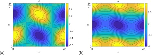
Figure 14. A typical unstable mode, with $B_0=0.05$, $\nu =\eta =0.1$, k = 0.5, from the flow or ${\Omega }_0$ branch; (a) shows the stream function ψ and (b) the magnetic potential a (Colour online).

The second system arising from perturbation theory involves $A_0$ and not ${\Omega }_0$: it is dominated by a large-scale magnetic field and so we refer to this as the $A_0$ or field branch of horizontal field instability. The result of perturbation theory gives (A.37(A.37) $p=(\frac{P}{2\nu }\frac{-{\nu }^2+3B_0^{2}P}{{\nu }^2+B_0^{2}P}-\frac{\nu }{P})k^2+\cdots .$(A.37) ), reproduced here as (51) $p=[\frac{P}{2\nu }\frac{-{\nu }^2+3B_0^{2}P}{{\nu }^2+B_0^{2}P}-\frac{\nu }{P}]k^2+\cdots \equiv -{\eta }_E{k}^2+\cdots .$(51) The onset of instability again can be interpreted as a transport quantity becoming negative; since $\eta =\nu /P$, for the field branch we can identify the instability as driven by a negative effective magnetic diffusivity ${\eta }_E$ (see Chechkin 1999). Note that this instability, being a directly growing instability, is not connected with the strong-field branch of the vertical field (which is an over-stable wave).

The threshold for instability is found by setting $-{\eta }_E$, namely the quantity in brackets in (51(51) $p=[\frac{P}{2\nu }\frac{-{\nu }^2+3B_0^{2}P}{{\nu }^2+B_0^{2}P}-\frac{\nu }{P}]k^2+\cdots \equiv -{\eta }_E{k}^2+\cdots .$(51) ), to zero giving (52) $B_0^2=\frac{{\nu }^2}{P}\frac{P^2+2{\nu }^2}{3P^2-2{\nu }^2}.$(52) The curve for $B_0(\nu ,P)$ is plotted on figure 13(b) in red and again shows good agreement with the numerical results for the field branch in panel (a). Note that for fixed P, $B_0\to \mathrm{\infty }$ as $\nu \to {\nu }_{\ast }$ with (53) ${\nu }_{\ast }=P\sqrt{3/2},$(53) and so a viscosity larger than this is enough to prevent the field branch instability no matter how strong the field. To confirm this, panels (c, d) of figure 13 show the same plots as panels (a, b) but over larger scales: the asymptote in (53(53) ${\nu }_{\ast }=P\sqrt{3/2},$(53) ), which is ${\nu }_{\ast }\simeq 1.225$ for P = 1, is evident and there is good agreement between theory and numerical calculations.

We also have for small fields and viscosities that the threshold (52(52) $B_0^2=\frac{{\nu }^2}{P}\frac{P^2+2{\nu }^2}{3P^2-2{\nu }^2}.$(52) ) is given by (54) $B_0\simeq \frac{\nu }{\sqrt{3P}},\nu \to 0,$(54) and so for P = 1 both thresholds (50(50) $B_0\simeq \frac{\nu }{P\sqrt{2+P}},\nu \to 0,$(50) ) and (54(54) $B_0\simeq \frac{\nu }{\sqrt{3P}},\nu \to 0,$(54) ) emerge from the origin with the same slope, though for general P the slopes are different. A typical example of the unstable fields is given in figure 15. The perturbation flow now does not have a zonostrophic jet structure, but shows closed eddies in panel (a) with significant ${\Psi }_{\pm 1}$ components. Panel (b) however shows a banded structure in the magnetic field showing the dominant role of the horizontal $A_0$ component. This indicates a tendency for the background mean field to segregate into bands of stronger and weaker zonal field, allowing the field mode to be identified also as a tearing mode (cf. Pessah 2010). Some comments on energetics of the two instability branches are given in Appendix A.4.

Figure 15. A typical unstable mode, with $B_0=0.25$, $\nu =\eta =0.1$, k = 0.25 from the field or $A_0$ branch; (a) shows the stream function ψ and (b) the magnetic potential a (Colour online).

We have explored the instabilities numerically for other values of P with $0.1\le P\le 10$ for $0.1\le \nu \le 1.0$ and various ranges of $B_0$, but will not present further figures here. For P decreasing from 1 down to 0.1 we observe only direct instability ($\mathrm{Im}\{p_{max}\}=0$) and the flow and field branches show good agreement with theory. For P increasing from 1 we again observe the (direct) flow and field branches accurately outlined by the theoretical curves. However a small but dominant island of oscillatory instabilities emerges from small values of ν and $B_0$ for P = 2 and spreads out in the vicinity of the lines (50(50) $B_0\simeq \frac{\nu }{P\sqrt{2+P}},\nu \to 0,$(50) ) and (54(54) $B_0\simeq \frac{\nu }{\sqrt{3P}},\nu \to 0,$(54) ). These instabilities have $k_{max}$ around 0.5 and are not captured by our perturbation expansions; we will leave these open to future exploration.

5.2. Instability for Bloch wave number $\ell \ne 0$

Finally, we consider horizontal field for the case of non-zero ℓ. This allows an instability to take up a scale $2\pi /k$ in the y-direction and $2\pi /\ell$, as $\ell \to 0$, in the x-direction. It turns out that instabilities can occur for $\ell \ne 0$ even when the system is stable for $\ell =0$, in the case of horizontal field (unlike the situation for vertical field).

Results are shown in figure 16 in which the maximisation in (27(27) $\mathrm{Re}\{p_{max}(\nu ,B_0,P,U_0)\}=\underset{k,\ell }{max}\mathrm{Re}\{p(k,\ell ,\nu ,B_0,P,U_0)\},$(27) ) is taken over a range of k and ℓ values including $\ell =0$; this should be compared with the earlier figure 13(a), which uses identical parameter ranges to show instabilities with ℓ constrained to be zero. The new figure 16 indicates considerable further structure across the four panels: depicted are (a, b) the real and imaginary parts of the growth rate $p_{max}$ and (c, d) the maximising values $k_{max}$ and ${\ell }_{max}$. We discuss the different regions in turn with reference to the white markers in each colour plot. First note that the prominent white curve in figure 13(a), as usual given by $\mathrm{Re}\{p_{max}\}=0$, has all but disappeared from the corresponding figure 16(a). Instead of clearly demarcating the flow and field instabilities as it does in figure 13(a), the white curve is reduced to a small triangle at the top right corner of figure 16(a), meaning that nearly the whole of the parameter space shown is unstable when $\ell \ne 0$ is allowed.

Figure 16. (a) Instability growth rate $\mathrm{Re}\{p_{max}\}$ and (b) imaginary part $\mathrm{Im}\{p_{max}\}$ shown for horizontal field, plotted in the $(\nu ,B_0)$ plane with P = 1, $U_0=0$, any ℓ and $0.1\le \nu \le 1$. The maximising values of $k_{max}$ and of ${\ell }_{max}$ are shown in panels (c, d), respectively. White markers indicate different regions of the diagrams as discussed in the text (Colour online).

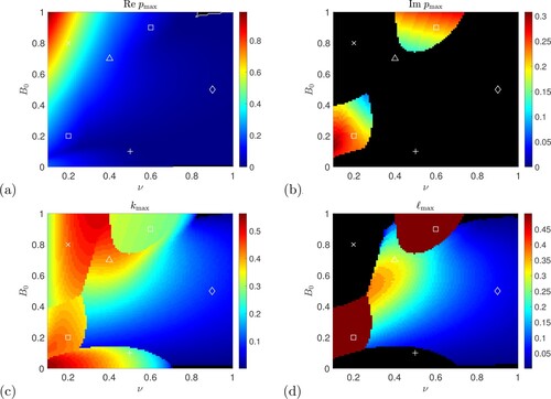
The flow or ${\Omega }_0$ branch clearly seen in the earlier $\ell =0$ figure 13(a), is still present in figure 16, near “+” at $(\nu ,B_0)=(0.5,0.1)$; because of low growth rates it is not really visible in figure 16(a) but is in figure 16(c) showing $k_{max}$. The field or $A_0$ branch in the $\ell =0$ figure 13(a) remains prominent in figure 16(a) (see “×” at $(\nu ,B_0)=(0.2,0.8)$), and near this point the dominant mode has ${\ell }_{max}=0$, from figure 16(d). However if we move rightwards then there is a transition seen in figure 16(d) from ${\ell }_{max}=0$ for the dominant modes, to ${\ell }_{max}\ne 0$, for example in the region around “$\mathrm{△}$”, $(\nu ,B_0)=(0.4,0.7)$. We also gain two new islands of instability attached to the field branch around the points marked by “□”, $(\nu ,B_0)=(0.2,0.2)$, $(0.6,0.9)$, having constant ${\ell }_{max}=0.5$ visible in figure 16(d), and so $4\pi$ periodicity in x; these also have non-zero frequency $\mathrm{Im}\{p_{max}\}$ in figure 16(c) and are further investigated in Algatheem (2023).

Finally we now gain a broad region of instability in figure 16(a) around “⋄”, $(\nu ,B_0)=(0.9,0.5)$ (which appears to be a smooth extension of the region around “$\mathrm{△}$” discussed above). This region was stable in the earlier figure 13(a) and so these modes are reliant on $\ell \ne 0$ for their existence. The modes have small values of $k_{max}$ and ${\ell }_{max}$ and low growth rates, but nonetheless their presence destabilises almost all of the stable region in the earlier figure 13(a), pushing the white curve in figure 16(a) to the top right corner for a tiny remnant region of stability. To gain further information about this new region of instability for $\ell \ne 0$ we therefore turn to theory for $\ell \ll 1$, $k\ll 1$, developed in Appendix D, which gives a growth rate in (D.12(D.12) $p=\pm B_0\ell {[\frac{k^2}{{\ell }^2+k^2}\frac{\mathrm{\nu \eta }+2{\eta }^2-B_0^2}{{\eta }^2(\mathrm{\nu \eta }+B_0^2)}-1]}^{1/2}+\cdots .$(D.12) ) of (55) $p=\pm B_0\ell {[\frac{k^2}{{\ell }^2+k^2}\frac{P[{\nu }^2(P+2)-P^2{B}_0^2]}{{\nu }^2({\nu }^2+P{B}_0^2)}-1]}^{1/2}+\cdots .$(55) This approximation reveals an instability that crucially relies on having a non-zero Bloch wavenumber, $\ell \ne 0$, with ℓ and k both small. If we fix the parameters ν, P and $B_0$ we can consider the growth rate p as a function in the $(\ell ,k)$ plane. Setting the quantity inside the square root to zero to find a threshold, we see that the region of instability is demarcated by the pair of straight lines given by (56) $\frac{k^2}{{\ell }^2}=\frac{{\nu }^2({\nu }^2+P{B}_0^2)}{{\nu }^2(P^2+2P-{\nu }^2)-P{B}_0^2({\nu }^2+P^2)}.$(56) The formula (55(55) $p=\pm B_0\ell {[\frac{k^2}{{\ell }^2+k^2}\frac{P[{\nu }^2(P+2)-P^2{B}_0^2]}{{\nu }^2({\nu }^2+P{B}_0^2)}-1]}^{1/2}+\cdots .$(55) ) for p tells us about the instability growth rate as we increase k and ℓ from zero, but to find how this eventually decreases, we would need to go to next order in perturbation theory, which is impractical and unlikely to be informative. To give a qualitative feel for the growth rate we will add on the diffusive suppression term $-\frac{1}{2}(\nu +\eta )(k^2+{\ell }^2)$ that is certainly one of those present at next order, and look at (57) $\begin{array}{rl}p& =\pm B_0\ell {[\frac{k^2}{{\ell }^2+k^2}\frac{P[{\nu }^2(P+2)-P^2{B}_0^2]}{{\nu }^2({\nu }^2+P{B}_0^2)}-1]}^{1/2}-\frac{1}{2}\nu (1+P^{-1})(k^2+{\ell }^2)\\ & +\mathrm{O}(k^2,{\ell }^2),\end{array}$(57) as a simple but crude approximation to $p(\ell ,k)$.

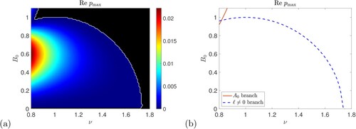
To see how all this fits together, figure 17(a) shows growth rates $\mathrm{Re}\{p(\ell ,k)\}$ obtained numerically and plotted in the $(\ell ,k)$-plane for $B_0=0.2$ and $\nu =\eta =0.75$. These parameters correspond to stability for $\ell =0$ as is evident from figure 13(a), the point $(0.75,0.2)$ lying in the black, stable region, but unstable for $\ell \ne 0$ from figure 16(a). The growth rate colour plot in figure 17(a) shows instability occuring for all $(\ell ,k)$ points lying inside the region taking a “butterfly” form, outlined by the white curves $\mathrm{Re}\{p\}=0$. These curves are tangential to the vertical axis $\ell =0$ at the origin, confirming that the modes with $\ell =0$ are stable for any k. The maximum instability growth rate here occurs for $(\ell ,k)\simeq (0.05,0.05)$.

Figure 17. Instability growth rate p for horizontal field as a function of $(\ell ,k)$ for $\nu =\eta =0.75$ (P = 1) with $B_0=0.2$, (a) numerical growth rates and (b) approximate growth rates calculated from (57(57) $\begin{array}{rl}p& =\pm B_0\ell {[\frac{k^2}{{\ell }^2+k^2}\frac{P[{\nu }^2(P+2)-P^2{B}_0^2]}{{\nu }^2({\nu }^2+P{B}_0^2)}-1]}^{1/2}-\frac{1}{2}\nu (1+P^{-1})(k^2+{\ell }^2)\\ & +\mathrm{O}(k^2,{\ell }^2),\end{array}$(57) ). In both panels the white curve is given by $\mathrm{Re}\{p\}=0$, with instability inside this curve, and the straight black lines emerging from the origin are from the formula (56(56) $\frac{k^2}{{\ell }^2}=\frac{{\nu }^2({\nu }^2+P{B}_0^2)}{{\nu }^2(P^2+2P-{\nu }^2)-P{B}_0^2({\nu }^2+P^2)}.$(56) ).

To compare with theory based on k, $\ell \to 0$, the straight black lines in figure 17(a) are given by (56(56) $\frac{k^2}{{\ell }^2}=\frac{{\nu }^2({\nu }^2+P{B}_0^2)}{{\nu }^2(P^2+2P-{\nu }^2)-P{B}_0^2({\nu }^2+P^2)}.$(56) ) and are tangential to the white curves at the origin, showing good agreement. In panel (b) we show an analogous figure for the “fixed up” growth rate in (57(57) $\begin{array}{rl}p& =\pm B_0\ell {[\frac{k^2}{{\ell }^2+k^2}\frac{P[{\nu }^2(P+2)-P^2{B}_0^2]}{{\nu }^2({\nu }^2+P{B}_0^2)}-1]}^{1/2}-\frac{1}{2}\nu (1+P^{-1})(k^2+{\ell }^2)\\ & +\mathrm{O}(k^2,{\ell }^2),\end{array}$(57) ). The agreement between the results in the two panels (a) and (b) is excellent near the origin, but then further out the agreement is only qualitative, and quite rough, as we might expect. This is because the term $-\frac{1}{2}\nu (1+P^{-1})(k^2+{\ell }^2)$ included in (57(57) $\begin{array}{rl}p& =\pm B_0\ell {[\frac{k^2}{{\ell }^2+k^2}\frac{P[{\nu }^2(P+2)-P^2{B}_0^2]}{{\nu }^2({\nu }^2+P{B}_0^2)}-1]}^{1/2}-\frac{1}{2}\nu (1+P^{-1})(k^2+{\ell }^2)\\ & +\mathrm{O}(k^2,{\ell }^2),\end{array}$(57) ) is only one of many which would appear by rigorous perturbation theory at order $k^2$, ${\ell }^2$, 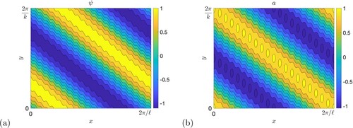and which would have a further stabilising effect in this case, judging by the figure. For an example of an unstable configuration, figure 18 shows the flow and field for the fastest growing mode in figure 17. We observe what we could term oblique zonostrophic instability: the emergence of a large-scale jet-like structure but at an oblique angle to the y-direction, this being allowed by the non-zero Bloch wavenumber ℓ.

Figure 18. A typical unstable mode, with $\ell =0.05$, k = 0.05, $\nu =\eta =0.75$, $B_0=0.2$; (a) shows the stream function ψ and (b) the magnetic potential a.

Returning to the bigger picture, for instability at a general point in the $(\nu ,B_0)$ plane we need the quantity inside the square root in (55(55) $p=\pm B_0\ell {[\frac{k^2}{{\ell }^2+k^2}\frac{P[{\nu }^2(P+2)-P^2{B}_0^2]}{{\nu }^2({\nu }^2+P{B}_0^2)}-1]}^{1/2}+\cdots .$(55) ) to be positive for some values of k and ℓ. Equivalently, it corresponds to requiring that the straight lines in (56(56) $\frac{k^2}{{\ell }^2}=\frac{{\nu }^2({\nu }^2+P{B}_0^2)}{{\nu }^2(P^2+2P-{\nu }^2)-P{B}_0^2({\nu }^2+P^2)}.$(56) ) have a finite slope. It can be checked that this gives a threshold for instability: (58) $B_0^2=\frac{{\nu }^2}{P}\frac{P(P+2)-{\nu }^2}{P^2+{\nu }^2}.$(58) Positive values of field smaller than this give instability and so this formula gives the threshold curve in the $(\nu ,B_0)$ plane for this family of $\ell \ne 0$ instabilities. This threshold is shown as a dashed curve in figure 13(b): we have instability to $\ell \ne 0$ modes below the dashed curve and we still have instability to $\ell =0$ modes above the red curve. We thus see in this panel that allowing any value of ℓ means that almost the whole of the parameter ranges shown give instability, all except for a small curved triangular region at the top right, and this is in agreement with the white curve obtained numerically in figure 16(a). The agreement is not perfect because the growth rates in the top right corner become small and the unstable region shrinks away in the $(\ell ,k)$-plane, as the thresholds are approached, and so the precise location of the white curve becomes hard to resolve without further work. Note that the formula (58(58) $B_0^2=\frac{{\nu }^2}{P}\frac{P(P+2)-{\nu }^2}{P^2+{\nu }^2}.$(58) ) does not capture the $\ell =0.5$ instability islands seen in figure 16; all the theory we have developed involves seeking instability by determining where the growth rate p can be positive in the limits $k\ll 1$ and $\ell \ll 1$. These islands are not detected by this means as they appear not to be connected to instability in this long-wavelength limit. As we found in the case of vertical field, theory for $k\to 0$ and/or $\ell \to 0$ gives sufficient conditions for instability, but does not rule out further instabilities.

Note that for P = 1, from (58(58) $B_0^2=\frac{{\nu }^2}{P}\frac{P(P+2)-{\nu }^2}{P^2+{\nu }^2}.$(58) ) the $\ell \ne 0$ instability is cut off at ${\nu }_{\ast }=\sqrt{3}$, and in general the instability requires (59) $\nu <{\nu }_{\ast }=\sqrt{P(2+P)}.$(59) Numerical experimentation, for cases where only the $\ell \ne 0$ instability is present, shows that for ν less than this threshold, the region of instability in the $(\ell ,k)$-plane becomes vanishingly small as $B_0$ tends to zero or tends to the value given in (58(58) $B_0^2=\frac{{\nu }^2}{P}\frac{P(P+2)-{\nu }^2}{P^2+{\nu }^2}.$(58) ). The maximum magnetic field for the $\ell \ne 0$ instability found here is given by maximising $B_0$ in (58(58) $B_0^2=\frac{{\nu }^2}{P}\frac{P(P+2)-{\nu }^2}{P^2+{\nu }^2}.$(58) ) over ν: the maximum occurs at (60) ${\nu }^2=-P^2+\sqrt{2P^3(1+P)}.$(60) To further confirm this analysis, figure 19 shows similar information to figure 16, but over a larger scale; the dashed curve in panel (b) shows the $\ell \ne 0$ threshold in (58(58) $B_0^2=\frac{{\nu }^2}{P}\frac{P(P+2)-{\nu }^2}{P^2+{\nu }^2}.$(58) ) and there is clear agreement between this and the numerical results in panel (a), in particular the ${\nu }_{\ast }=\sqrt{3}\simeq 1.73$ threshold for P = 1. We make additional points in the final discussion section 6.

Figure 19. (a) Instability growth rate $\mathrm{Re}\{p_{max}\}$ plotted in the $(\nu ,B_0)$ plane with P = 1, $U_0=0$, and $\ell \ne 0$; (b) shows thresholds (52(52) $B_0^2=\frac{{\nu }^2}{P}\frac{P^2+2{\nu }^2}{3P^2-2{\nu }^2}.$(52) ) for $\ell =0$ (red) and (58(58) $B_0^2=\frac{{\nu }^2}{P}\frac{P(P+2)-{\nu }^2}{P^2+{\nu }^2}.$(58) ) for $\ell \ne 0$ (blue dashed) (Colour online).

6. Discussion

In this study we have explored instability of the classic Kolmogorov flow in the presence of magnetic field which is either vertical, aligned with the flow, or horizontal, aligned with possible jet formation. In the first case we have obtained new analytical results for the maximum growth rate (30(30) $p_{max}(\nu ,B_0,P)=-\frac{\sqrt{2}P}{1+P^2}{B}_0^2+\frac{\sqrt{2}}{3}(\frac{1}{\sqrt{2}}-\nu {)}^2,k_{max}^2=\frac{\sqrt{2}}{3}(\frac{1}{\sqrt{2}}-\nu ).$(30) ) and magnetic field threshold (31(31) $B_0(\nu ,P)=\sqrt{\frac{1+P^2}{3P}}(\frac{1}{\sqrt{2}}-\nu ).$(31) ), that show the suppression of the original zonostrophic instability found by Meshalkin and Sinai (1961) by vertical magnetic field. For the strong field branch, present when P<1, we have confirmed the numerical results of Fraser et al. (2022) and provided an alternative derivation of their growth rate formula (33(33) $\mathrm{Re}\{p\}=\frac{\frac{1}{4}\mathrm{\nu \eta }(\eta -\nu )k^2}{{\nu }^2{\eta }^2+k^2{B}_0^2(\nu +\eta {)}^2}-\frac{1}{2}(\nu +\eta )k^2+\cdots .$(33) ) and threshold (35(35) $\nu <{\nu }_{\ast }=\sqrt{\frac{P}{2}\frac{1-P}{1+P}}\mathrm{or}R>R_{\ast }=\sqrt{\frac{2}{P}\frac{1+P}{1-P}}.$(35) ), generalised to non-zero mean flow $U_0$ in (B.16(B.16) $p=\frac{1}{4}\Delta (\eta -\nu )[\mathrm{\nu \eta }+\mathrm{i}k{B}_0(\nu +\eta )-U_0^2]k^2-\frac{1}{2}(\nu +\eta )k^2+\cdots ,$(B.16) ) and (39(39) $\frac{P}{2}\frac{1-P}{1+P}({\nu }_{\ast }^2-P{U}_0^2)=({\nu }_{\ast }^2+U_0^2)({\nu }_{\ast }^2+P^2{U}_0^2).$(39) ). We have presented numerical results showing how such a mean flow $U_0>0$ can suppress the hydrodynamic threshold (i.e. for $B_0=0$) in (36(36) ${\nu }_c(U_0)=\sqrt{\frac{1}{2}-U_0^2},\mathrm{for}{U}_0<1/\sqrt{2},B_0=0,$(36) ) and the weak field branch of instability (for $B_0>0$), modify thresholds ${\nu }_{\ast }$ for the P<1 strong field branch in (39(39) $\frac{P}{2}\frac{1-P}{1+P}({\nu }_{\ast }^2-P{U}_0^2)=({\nu }_{\ast }^2+U_0^2)({\nu }_{\ast }^2+P^2{U}_0^2).$(39) ), and lead to a new branch of instabilities for P>1. We note that Fraser et al. (2022) also find a further branch of instabilities for $P\ge 1$, which they term “varicose Kelvin–Helmholtz” modes, from Reynolds numbers of the order of a hundred. This branch is not visible in our figures since in our scans of the $(\nu ,B_0)$ parameter space we have cut off ν at a value of 0.01 or 0.1 (for vertical or horizontal field, respectively), as detailed in each figure caption.

The case of horizontal field, broadly relevant to several studies of jet formation where the field is aligned with potential jets (Tobias et al. 2007, Durston and Gilbert 2016, Constantinou and Parker 2018), shows more complex structure, unsurprisingly given the wavey nature of the magnetic field in the basic state, seen in figure 1(b). Nonetheless, theory based on large-scale perturbations with $k\ll 1$, $\ell \ll 1$, although only sufficient for instability, in reality gives a good guide to most (although not all) of what we have found numerically. We observe again the suppression of the purely hydrodynamic zonostrophic instability, the flow or ${\Omega }_0$ branch, when the magnetic field strength is increased. A similar effect is seen in the shear layer/jet configuration of Lewis (2022). The threshold of $B_0=B_{\ast }$ for complete suppression is given by substituting ${\nu }^2$ from (49(49) $2{\nu }^2=-Q+\sqrt{Q^2+Q},Q=2P+P^2,$(49) ) into (48(48) $B_0^2=\frac{{\nu }^2}{P}\frac{1-2{\nu }^2}{P(P+2)+2{\nu }^2}.$(48) ). For large P, we have ${\nu }^2\simeq 1/4$ while for small P, ${\nu }^2\simeq \sqrt{P/2}$. The value of $B_{\ast }$ for suppression then amounts to: (61) $B_{\ast }^2\sim P^{-1}=\frac{\eta }{\nu }(P\ll 1),B_{\ast }^2\sim P^{-3}=\frac{{\eta }^3}{{\nu }^3}(P\gg 1).$(61) Interestingly this bears comparison with Tobias et al. (2007) who have $\nu ={10}^{-4}$ fixed and ${10}^{-1}\le \eta \le {10}^{-6}$ in their runs. For the greater values of η used, $P\ll 1$ and so a threshold $B_{\ast }^2\sim \eta$ is indicated above, and found in these full numerical simulations. Also, note that at this threshold we have that the forcing magnitude is fixed in magnitude in (40(40) ${\mathit{u}}_0=(0,\sin x),{\mathit{b}}_0=(B_0,{\eta }^{-1}{B}_0\cos x),\mathit{f}=(0,(\nu +{\eta }^{-1}{B}_0^2)\sin x),$(40) ) and so there is, at least roughly, a correspondence of working with fixed forcing amplitude as in their paper and the fixed Kolmogorov flow in ours. However we should remark that these authors use a stochastic, ring forcing and a non-zero value of β, whereas we have a steady forcing and have taken ℓ to be zero; thus further work would be needed to make a sound comparison.

A feature of the horizontal field problem is that for increasing magnetic field strengths a further branch of instabilities emerges, the field or $A_0$ branch, also seen in Durston and Gilbert (2016) and by Lewis (2022) in the shear layer/jet geometry; these may be identified as tearing modes. An analytical formula (52(52) $B_0^2=\frac{{\nu }^2}{P}\frac{P^2+2{\nu }^2}{3P^2-2{\nu }^2}.$(52) ) for the threshold of instability is given for this branch, which exists provided the Reynolds number satisfies $R>{\nu }_{\ast }^{-1}$ with ${\nu }_{\ast }$ given in (53(53) ${\nu }_{\ast }=P\sqrt{3/2},$(53) ). Allowing a Bloch wavenumber $\ell \ne 0$ in the x-direction, in addition to the wavenumber k in the y-direction, allows a new branch of instabilities, which we have categorised as oblique zonostrophic instabilities. In particular a magnetic field, no matter how weak, can destabilise the Kolmogorov flow provided the Reynolds number $R={\nu }^{-1}>{\nu }_{\ast }^{-1}$ with ${\nu }_{\ast }$ given in (59(59) $\nu <{\nu }_{\ast }=\sqrt{P(2+P)}.$(59) ). For example at P = 1, the purely hydrodynamic instability is present for $R>\sqrt{2}$ but the oblique instability is present for arbitrarily weak but non-zero horizontal magnetic field provided $R>1/\sqrt{3}$. For sufficiently large magnetic field this instability is again suppressed, and making use of (60(60) ${\nu }^2=-P^2+\sqrt{2P^3(1+P)}.$(60) ) (with ${\nu }^2\simeq \sqrt{2P^3}$ for small P and ${\nu }^2\simeq (\sqrt{2}-1)P^2$ for large P) we find a threshold (62) $B_{\ast }^2\sim 1(P\ll 1),B_{\ast }^2\sim P=\frac{\nu }{\eta }(P\gg 1).$(62) Note that the order of limits could be important: in our discussion in this paper we are fixing any value of P and then allowing k and ℓ to tend to zero. Other limits are possible and could be explored by appropriate scalings in our calculations. We stress again that all our theory is based on the limits $k\to 0$, $\ell \to 0$, and further instabilities can occur that have no connection with this limit, as we have seen repeatedly. Our theoretical criteria for instability are always sufficient but not necessary, and while we have given some numerical surveys, the complete parameter space of $\{\nu ,P,B_0,U_0\}$ is large once one allows both k and ℓ to be non-zero. It can be enlarged further by including a β-effect of general orientation (Manfroi and Young 2002) or an arbitrary angle γ of the imposed magnetic field $B_0$ in the $(x,y)$-plane (further studied in Algatheem 2023), generalisations open to future investigation.

Underlying our study is matrix eigenvalue perturbation theory as set out in the appendices, a flexible tool for these types of problems. We find it gives greater clarity than using a multiple scales formulation or applying perturbation theory to roots of a polynomial, even though all these methods are ultimately equivalent for linear theory. Note that while many of the instabilities seen by us and by other authors can be characterised as involving a negative effective viscosity term, $-{\nu }_E{k}^2$ with ${\nu }_E<0$, or a negative effective magnetic diffusivity term, $-{\eta }_E{k}^2$ with ${\eta }_E<0$, at large scales, the growth rate $p(k,\ell )$ in the case of horizontal field shows a complicated dependence on k and ℓ in (55(55) $p=\pm B_0\ell {[\frac{k^2}{{\ell }^2+k^2}\frac{P[{\nu }^2(P+2)-P^2{B}_0^2]}{{\nu }^2({\nu }^2+P{B}_0^2)}-1]}^{1/2}+\cdots .$(55) ). Although this $\ell \ne 0$ instability occurs at arbitrarily large scales, it cannot be categorised as involving a simple negative effective transport effect. This arises because we are applying perturbation theory to a repeated eigenvalue of the limiting $k\to 0$, $\ell \to 0$ problem. Looking to the future, it would be interesting to pursue further research on the Kolmogorov flow as an MHD system, particularly on the nonlinear evolution of instabilities and inverse cascades (Fraser et al. 2022, Algatheem 2023), and on the interaction of magnetic field with a β-effect and Rossby waves.

Acknowledgments

We are most grateful to the referees for their careful reading and critique of the original manuscript, which led to corrections to our original discussion of the weak field branch behaviour for large P, further work on the role of $U_0$, and useful additional references. We would also like to thank Adrian Fraser and Chen Wang for useful discussions and references. For the purpose of open access, the authors have applied a Creative Commons Attribution (CC BY) licence to any Author Accepted Manuscript version arising.

Disclosure statement

No potential conflict of interest was reported by the authors.

Data access statement

Sample Matlab scripts, those used to generate figures 2, 3 and 5, have been lodged in Github under https://github.com/Algatheem/Matlab-code-GAFD-paper-2023. Further scripts are available from the authors, following any reasonable request.

Additional information

Funding

ADG acknowledges support from the EPSRC Research Grant EP/T023139/1 and AH support from the STFC Research Grant ST/V000659/1. AMA is thankful to the Deanship of Scientific Research at the University of Bisha for financial support through the Scholars Research Support Programme of the university.

Notes

1 We use the term “effective viscosity” ${\nu }_E$ but really this quantity involves the viscosity and the magnetic diffusion on an equal basis, as per the sub-expression $\frac{1}{2}(\nu +\eta )k^2$; it is perhaps better described as an effective Alfvén wave damping rate, in other words a modification to (28(28) $p=\pm \mathrm{i}k\sqrt{B_0^2-\frac{1}{4}(\nu -\eta {)}^2{k}^2}-\frac{1}{2}(\nu +\eta )k^2,$(28) ).

2 Further investigation (which we will not detail here) indicates that at, for example $B_0=0.25$ (dark orange curve in figure 12(a)), when k is increased from zero the leading real eigenvalue corresponding to the first peak collides at $k\simeq 0.35$ with another, subdominant real eigenvalue. To the right of this collision, these two real branches merge to give two complex eigenvalues that form the second peak. For this second peak the structure of field and flow is similar to that in figure 15 below for the first peak, but up–down symmetry is lost in each of the pair of complex eigenmodes.

3 We note that this approach is equivalent to quasi-linear theory for weak large-scale (or mean) fields. In our set-up the n = 0, $k\ll 1$ mode can be identified with a large-scale magnetic field and flow, and at first order we are solving for the $n=\pm 1$ fluctuations on the flow generated by the forcing that maintains the Kolmogorov flow. Calculating the second-order feedback on the n = 0 mode in perturbation theory, which can have a destablising effect, is equivalent to evaluating the mean quadratic terms in quasi-linear theory.

Appendix A.

Horizontal field, with $U_0=0$, $\ell =0$

First, let us outline the general principles of our approximate analysis of growth rates in this and other appendices. In each case we have an infinite system of coupled linear equations, for example (45(45) $\begin{array}{rl}p{\Omega }_n& =-\nu (n^2+k^2){\Omega }_n+\frac{k}{2}(\frac{1}{(n-1{)}^2+k^2}-1){\Omega }_{n-1}\\ & -\frac{k}{2}(\frac{1}{(n+1{)}^2+k^2}-1){\Omega }_{n+1}\\ & +\mathrm{i}n{B}_0(n^2+k^2)A_n+\frac{\mathrm{i}k{B}_0}{2\eta }[(n-1{)}^2+k^2-1]A_{n-1}\\ & +\frac{\mathrm{i}k{B}_0}{2\eta }[(n+1{)}^2+k^2-1]A_{n+1},\end{array}$(45) ), (46(46) $\begin{array}{rl}p{A}_n& =-\eta (n^2+k^2)A_n-\frac{k}{2}{A}_{n-1}+\frac{k}{2}{A}_{n+1}\\ & +\frac{\mathrm{i}n{B}_0}{n^2+k^2}{\Omega }_n+\frac{\mathrm{i}k{B}_0}{2\eta }\frac{1}{(n-1{)}^2+k^2}{\Omega }_{n-1}+\frac{\mathrm{i}k{B}_0}{2\eta }\frac{1}{(n+1{)}^2+k^2}{\Omega }_{n+1},\end{array}$(46) ) in the case of horizontal field with $U_0=0$ and $\ell =0$. In the limit $k\to 0$ of large-scale modes, we can reduce the calculation of the growth rate to eigenvalues of a finite matrix. The key point to note is that the n = 0 modes ${\Omega }_0$ and $A_0$ are distinguished from all other modes by being weakly damped, as $p_{\mathrm{visc}}=-\nu k^2$ or $p_{\mathrm{diff}}=-\eta k^2$ by molecular diffusion with $k\ll 1$. On the other hand other modes with $|n|>0$ are relatively strongly damped, with $p_{\mathrm{visc}}=-\nu (n^2+k^2)$ or $p_{\mathrm{diff}}=-\eta (n^2+k^2)$. So we need to keep the n = 0 modes as these are most easily destabilised in the system. How are they destabilised? This is through the coupling from n = 0 to low $n\ne 0$ modes and then back to n = 0, and via these couplings the unstable fields can draw energy from the basic state Kolmogorov flow ${\mathit{u}}_0=(0,\sin x)$ or the varying component of the background magnetic field $(0,{\eta }^{-1}{B}_0\cos x)$ (in the horizontal case only). It then follows that we typically expect to see effects only at second order or beyond in terms of perturbation theory, and this will usually involve ${\Omega }_n$ and $A_n$ for n = −1, 0, 1 only.³ Thus we can truncate the system and then use perturbation theory for the eigenvalues of a finite matrix, with $k\ll 1$ as an expansion parameter.

Thus we set to work on the horizontal system of equations (45(45) $\begin{array}{rl}p{\Omega }_n& =-\nu (n^2+k^2){\Omega }_n+\frac{k}{2}(\frac{1}{(n-1{)}^2+k^2}-1){\Omega }_{n-1}\\ & -\frac{k}{2}(\frac{1}{(n+1{)}^2+k^2}-1){\Omega }_{n+1}\\ & +\mathrm{i}n{B}_0(n^2+k^2)A_n+\frac{\mathrm{i}k{B}_0}{2\eta }[(n-1{)}^2+k^2-1]A_{n-1}\\ & +\frac{\mathrm{i}k{B}_0}{2\eta }[(n+1{)}^2+k^2-1]A_{n+1},\end{array}$(45) ), (46(46) $\begin{array}{rl}p{A}_n& =-\eta (n^2+k^2)A_n-\frac{k}{2}{A}_{n-1}+\frac{k}{2}{A}_{n+1}\\ & +\frac{\mathrm{i}n{B}_0}{n^2+k^2}{\Omega }_n+\frac{\mathrm{i}k{B}_0}{2\eta }\frac{1}{(n-1{)}^2+k^2}{\Omega }_{n-1}+\frac{\mathrm{i}k{B}_0}{2\eta }\frac{1}{(n+1{)}^2+k^2}{\Omega }_{n+1},\end{array}$(46) ) in Fourier space. These are truncated to just the modes ${\Omega }_0$, ${\Omega }_{\pm 1}$, $A_0$ and $A_{\pm 1}$, with (A.1) $\begin{array}{rl}p{\Omega }_0& =-\nu k^2{\Omega }_0-\frac{k}{2}\frac{k^2}{1+k^2}{\Omega }_{-1}+\frac{k}{2}\frac{k^2}{1+k^2}{\Omega }_1+\frac{\mathrm{i}k{B}_0}{2\eta }{k}^2{A}_{-1}+\frac{\mathrm{i}k{B}_0}{2\eta }{k}^2{A}_1,\end{array}$(A.1) (A.2) $\begin{array}{rl}p{A}_0& =-\eta k^2{A}_0-\frac{k}{2}{A}_{-1}+\frac{k}{2}{A}_1+\frac{\mathrm{i}k{B}_0}{2\eta }\frac{1}{1+k^2}{\Omega }_{-1}+\frac{\mathrm{i}k{B}_0}{2\eta }\frac{1}{1+k^2}{\Omega }_1,\end{array}$(A.2) (A.3) $\begin{array}{rl}p{\Omega }_{\pm 1}& =-\nu (1+k^2){\Omega }_{\pm 1}\pm \frac{k}{2}\frac{1-k^2}{k^2}{\Omega }_0\pm \mathrm{i}{B}_0(1+k^2)A_{\pm 1}+\frac{\mathrm{i}k{B}_0}{2\eta }(-1+k^2)A_0,\end{array}$(A.3) (A.4) $\begin{array}{rl}p{A}_{\pm 1}& =-\eta (1+k^2)A_{\pm 1}\mp \frac{k}{2}{A}_0\pm \mathrm{i}{B}_0\frac{1}{1+k^2}{\Omega }_{\pm 1}+\frac{\mathrm{i}k{B}_0}{2\eta }\frac{1}{k^2}{\Omega }_0.\end{array}$(A.4) We now express these equations in terms of ${\Omega }_0$, $A_0$ and the fields (A.5) ${\Omega }_{\pm }=\frac{1}{2}({\Omega }_1\pm {\Omega }_{-1}),A_{\pm }=\frac{1}{2}(A_1\pm A_{-1});$(A.5) we rescale ${\Omega }_0={\Omega }_0^{\prime }{k}^2$ and for convenience we set ${\tilde{B}}_0=B_0/\eta$. The resulting equations then break up into two uncoupled systems. The first involves only ${\Omega }_0^{\prime }$ on the large scale, (A.6) $\begin{array}{rl}p{\Omega }_0^{\prime }& =-\nu k^2{\Omega }_0^{\prime }+k(1+k^2{)}^{-1}{\Omega }_{-}+\mathrm{i}k{\tilde{B}}_0{A}_{+},\end{array}$(A.6) (A.7) $\begin{array}{rl}p{\Omega }_{-}& =-\nu (1+k^2){\Omega }_{-}+\frac{1}{2}k(1-k^2){\Omega }_0^{\prime }+\mathrm{i}{B}_0(1+k^2)A_{+},\end{array}$(A.7) (A.8) $\begin{array}{rl}p{A}_{+}& =-\eta (1+k^2)A_{+}+\mathrm{i}{B}_0(1+k^2{)}^{-1}{\Omega }_{-}+\frac{1}{2}\mathrm{i}k{\tilde{B}}_0{\Omega }_0^{\prime },\end{array}$(A.8) while the second involves only $A_0$ on the large scale, (A.9) $\begin{array}{rl}p{A}_0& =-\eta k^2{A}_0+k{A}_{-}+\mathrm{i}k{\tilde{B}}_0(1+k^2{)}^{-1}{\Omega }_{+},\end{array}$(A.9) (A.10) $\begin{array}{rl}p{A}_{-}& =-\eta (1+k^2)A_{-}-\frac{1}{2}k{A}_0+\mathrm{i}{B}_0(1+k^2{)}^{-1}{\Omega }_{+},\end{array}$(A.10) (A.11) $\begin{array}{rl}p{\Omega }_{+}& =-\nu (1+k^2){\Omega }_{+}+\mathrm{i}{B}_0(1+k^2)A_{-}+\frac{1}{2}\mathrm{i}k{\tilde{B}}_0(-1+k^2)A_0,\end{array}$(A.11) We deal with these two branches in turn, using eigenvalue perturbation theory.

A.1. Outline of approach

Having reduced the problem to the calculation of eigenvalues p for two systems of equations for $k\ll 1$, one for (A.6(A.6) $\begin{array}{rl}p{\Omega }_0^{\prime }& =-\nu k^2{\Omega }_0^{\prime }+k(1+k^2{)}^{-1}{\Omega }_{-}+\mathrm{i}k{\tilde{B}}_0{A}_{+},\end{array}$(A.6) )–(A.8(A.8) $\begin{array}{rl}p{A}_{+}& =-\eta (1+k^2)A_{+}+\mathrm{i}{B}_0(1+k^2{)}^{-1}{\Omega }_{-}+\frac{1}{2}\mathrm{i}k{\tilde{B}}_0{\Omega }_0^{\prime },\end{array}$(A.8) ) and one for (A.9(A.9) $\begin{array}{rl}p{A}_0& =-\eta k^2{A}_0+k{A}_{-}+\mathrm{i}k{\tilde{B}}_0(1+k^2{)}^{-1}{\Omega }_{+},\end{array}$(A.9) )–(A.11(A.11) $\begin{array}{rl}p{\Omega }_{+}& =-\nu (1+k^2){\Omega }_{+}+\mathrm{i}{B}_0(1+k^2)A_{-}+\frac{1}{2}\mathrm{i}k{\tilde{B}}_0(-1+k^2)A_0,\end{array}$(A.11) ), we outline the method that is common to all the approximations in the paper. In each case we write the governing eigenvalue problem in a matrix form (see (A.24(A.24) $M=\left(\begin{array}{ccc}-\nu k^2& k(1+k^2{)}^{-1}& \mathrm{i}k{\tilde{B}}_0\\ \frac{1}{2}k(1-k^2)& -\nu (1+k^2)& \mathrm{i}{B}_0(1+k^2)\\ \frac{1}{2}\mathrm{i}k{\tilde{B}}_0& \mathrm{i}{B}_0(1+k^2{)}^{-1}& -\eta (1+k^2)\end{array}\right),\mathit{v}=\left(\begin{array}{c}{\Omega }_0^{\prime }\\ {\Omega }_{-}\\ A_{+}\end{array}\right).$(A.24) ), (A.32(A.32) $M=\left(\begin{array}{ccc}-\eta k^2& k& \mathrm{i}k{\tilde{B}}_0(1+k^2{)}^{-1}\\ -\frac{1}{2}k& -\eta (1+k^2)& \mathrm{i}{B}_0(1+k^2{)}^{-1}\\ \frac{1}{2}\mathrm{i}k{\tilde{B}}_0(-1+k^2)& \mathrm{i}{B}_0(1+k^2)& -\nu (1+k^2)\end{array}\right),\mathit{v}=\left(\begin{array}{c}{A}_0\\ A_{-}\\ {\Omega }_{+}\end{array}\right).$(A.32) ) below) where the matrix M depends on k, $\mathit{v}$ is the eigenvector and p the eigenvalue: (A.12) $M\mathit{v}=p\mathit{v}.$(A.12) We may rescale some quantities in the matrix M (using a prime to denote these) and we then proceed to expand M in powers of k as (A.13) $M=M_0+k{M}_1+k^2{M}_2+\cdots ,$(A.13) and likewise $\mathit{v}$ and p. For the limit $k\to 0$ we solve (A.14) $(M_0+k{M}_1+\cdots )({\mathit{v}}_0+k{\mathit{v}}_1+\cdots )=(p_0+k{p}_1+\cdots )({\mathit{v}}_0+k{\mathit{v}}_1+\cdots ),$(A.14) order by order in k. Here we set out the first few orders in a convenient form: (A.15) $\begin{array}{rl}{p}_0{\mathit{v}}_0& =M_0{\mathit{v}}_0,\end{array}$(A.15) (A.16) $\begin{array}{rl}{p}_1{\mathit{v}}_0& =(M_0-p_0){\mathit{v}}_1+M_1{\mathit{v}}_0,\end{array}$(A.16) (A.17) $\begin{array}{rl}{p}_2{\mathit{v}}_0& =(M_0-p_0){\mathit{v}}_2+M_2{\mathit{v}}_0+M_1{\mathit{v}}_1-p_1{\mathit{v}}_1,\end{array}$(A.17) (A.18) $\begin{array}{rl}{p}_3{\mathit{v}}_0& =(M_0-p_0){\mathit{v}}_3+M_3{\mathit{v}}_0+M_2{\mathit{v}}_1+M_1{\mathit{v}}_2-p_2{\mathit{v}}_1-p_1{\mathit{v}}_2,\end{array}$(A.18) (A.19) $\begin{array}{rl}{p}_4{\mathit{v}}_0& =(M_0-p_0){\mathit{v}}_4+M_4{\mathit{v}}_0+M_3{\mathit{v}}_1+M_2{\mathit{v}}_2+M_1{\mathit{v}}_3-p_3{\mathit{v}}_1-p_2{\mathit{v}}_2-p_1{\mathit{v}}_3.\end{array}$(A.19) First we choose an eigenvalue $p_0$ and corresponding right (column) eigenvector ${\mathit{v}}_0$ of $M_0$; at the level of $M_0$ the mode is undamped and so the real part of $p_0$ is zero. Assuming this is a simple (non-repeated) eigenvalue there is also a single left (row) eigenvector ${\mathit{w}}_0$ with ${\mathit{w}}_0(M_0-p_0)=0$. With (A.15(A.15) $\begin{array}{rl}{p}_0{\mathit{v}}_0& =M_0{\mathit{v}}_0,\end{array}$(A.15) ) thus dealt with, we note that we gain successive eigenvalue terms $p_j$ from applying ${\mathit{w}}_0$ to the left of the remaining equations, so that (A.20) $\begin{array}{rl}{p}_1{\mathit{w}}_0{\mathit{v}}_0& ={\mathit{w}}_0{M}_1{\mathit{v}}_0,\end{array}$(A.20) (A.21) $\begin{array}{rl}{p}_2{\mathit{w}}_0{\mathit{v}}_0& ={\mathit{w}}_0(M_2{\mathit{v}}_0+M_1{\mathit{v}}_1-p_1{\mathit{v}}_1),\end{array}$(A.21) (A.22) $\begin{array}{rl}{p}_3{\mathit{w}}_0{\mathit{v}}_0& ={\mathit{w}}_0(M_3{\mathit{v}}_0+M_2{\mathit{v}}_1+M_1{\mathit{v}}_2-p_2{\mathit{v}}_1-p_1{\mathit{v}}_2),\end{array}$(A.22) (A.23) $\begin{array}{rl}{p}_4{\mathit{w}}_0{\mathit{v}}_0& ={\mathit{w}}_0(M_4{\mathit{v}}_0+M_3{\mathit{v}}_1+M_2{\mathit{v}}_2+M_1{\mathit{v}}_3-p_3{\mathit{v}}_1-p_2{\mathit{v}}_2-p_1{\mathit{v}}_3).\end{array}$(A.23) Here ${\mathit{w}}_0{\mathit{v}}_0$ is the scalar obtained by multiplying the row vector ${\mathit{w}}_0$ by the column vector ${\mathit{v}}_0$. In this way, once having chosen the eigenvalue $p_0$ to perturb from (A.15(A.15) $\begin{array}{rl}{p}_0{\mathit{v}}_0& =M_0{\mathit{v}}_0,\end{array}$(A.15) ) together with ${\mathit{v}}_0$ and ${\mathit{w}}_0$, we find $p_1$ from (A.20(A.20) $\begin{array}{rl}{p}_1{\mathit{w}}_0{\mathit{v}}_0& ={\mathit{w}}_0{M}_1{\mathit{v}}_0,\end{array}$(A.20) ). We then need ${\mathit{v}}_1$ from (A.16(A.16) $\begin{array}{rl}{p}_1{\mathit{v}}_0& =(M_0-p_0){\mathit{v}}_1+M_1{\mathit{v}}_0,\end{array}$(A.16) ) and while $M_0-p_0$ is not invertible, having fixed the value of $p_1$, there is a solution for ${\mathit{v}}_1$. It is not unique, but this does not matter as we shall see. We can then calculate $p_2$ from (A.21(A.21) $\begin{array}{rl}{p}_2{\mathit{w}}_0{\mathit{v}}_0& ={\mathit{w}}_0(M_2{\mathit{v}}_0+M_1{\mathit{v}}_1-p_1{\mathit{v}}_1),\end{array}$(A.21) ) and so forth. We will go up to the level of $p_4$ in some of our calculations below.

A.2. Flow or ${\Omega }_0$ branch

Having set out our general approach we return to the first system (A.6(A.6) $\begin{array}{rl}p{\Omega }_0^{\prime }& =-\nu k^2{\Omega }_0^{\prime }+k(1+k^2{)}^{-1}{\Omega }_{-}+\mathrm{i}k{\tilde{B}}_0{A}_{+},\end{array}$(A.6) )–(A.8(A.8) $\begin{array}{rl}p{A}_{+}& =-\eta (1+k^2)A_{+}+\mathrm{i}{B}_0(1+k^2{)}^{-1}{\Omega }_{-}+\frac{1}{2}\mathrm{i}k{\tilde{B}}_0{\Omega }_0^{\prime },\end{array}$(A.8) ), which involves a dominant large-scale flow in ${\Omega }_0$ and no large-scale field, with (A.24) $M=\left(\begin{array}{ccc}-\nu k^2& k(1+k^2{)}^{-1}& \mathrm{i}k{\tilde{B}}_0\\ \frac{1}{2}k(1-k^2)& -\nu (1+k^2)& \mathrm{i}{B}_0(1+k^2)\\ \frac{1}{2}\mathrm{i}k{\tilde{B}}_0& \mathrm{i}{B}_0(1+k^2{)}^{-1}& -\eta (1+k^2)\end{array}\right),\mathit{v}=\left(\begin{array}{c}{\Omega }_0^{\prime }\\ {\Omega }_{-}\\ A_{+}\end{array}\right).$(A.24) For this branch we expand M to give: (A.25) $M_0=\left(\begin{array}{ccc}0& 0& 0\\ 0& -\nu & \mathrm{i}{B}_0\\ 0& \mathrm{i}{B}_0& -\eta \end{array}\right),M_1=\left(\begin{array}{ccc}0& 1& \mathrm{i}{\tilde{B}}_0\\ \frac{1}{2}& 0& 0\\ \frac{1}{2}\mathrm{i}{\tilde{B}}_0& 0& 0\end{array}\right),M_2=\left(\begin{array}{ccc}-\nu & 0& 0\\ 0& -\nu & \mathrm{i}{B}_0\\ 0& -\mathrm{i}{B}_0& -\eta \end{array}\right).$(A.25) Note that the inverse of the non-trivial $2\times 2$ block of $M_0$ is (A.26) ${\left(\begin{array}{cc}-\nu & \mathrm{i}{B}_0\\ \mathrm{i}{B}_0& -\eta \end{array}\right)}^{-1}=\Delta \left(\begin{array}{cc}-\eta & -\mathrm{i}{B}_0\\ -\mathrm{i}{B}_0& -\nu \end{array}\right),{\Delta }^{-1}=\mathrm{\nu \eta }+B_0^2,$(A.26) where Δ is the inverse of the appropriate determinant.

We are ready to solve order by order in k. At leading order (A.15(A.15) $\begin{array}{rl}{p}_0{\mathit{v}}_0& =M_0{\mathit{v}}_0,\end{array}$(A.15) ) we choose (A.27) $p_0=0,{\mathit{v}}_0=(1,0,0{)}^T,{\mathit{w}}_0=(1,0,0).$(A.27) At next order, we use (A.20(A.20) $\begin{array}{rl}{p}_1{\mathit{w}}_0{\mathit{v}}_0& ={\mathit{w}}_0{M}_1{\mathit{v}}_0,\end{array}$(A.20) ) and have (A.28) $M_1{\mathit{v}}_0=(0,\frac{1}{2},\frac{1}{2}\mathrm{i}{\tilde{B}}_0{)}^T,p_1=0.$(A.28) Given this we now solve (A.16(A.16) $\begin{array}{rl}{p}_1{\mathit{v}}_0& =(M_0-p_0){\mathit{v}}_1+M_1{\mathit{v}}_0,\end{array}$(A.16) ) for ${\mathit{v}}_1$, to obtain (A.29) ${\mathit{v}}_1=\frac{1}{2}\Delta (0,\eta -{\tilde{B}}_0{B}_0,\mathrm{i}{B}_0+\mathrm{i}\nu {\tilde{B}}_0{)}^T.$(A.29) Here we have used the inverse (A.26(A.26) ${\left(\begin{array}{cc}-\nu & \mathrm{i}{B}_0\\ \mathrm{i}{B}_0& -\eta \end{array}\right)}^{-1}=\Delta \left(\begin{array}{cc}-\eta & -\mathrm{i}{B}_0\\ -\mathrm{i}{B}_0& -\nu \end{array}\right),{\Delta }^{-1}=\mathrm{\nu \eta }+B_0^2,$(A.26) ) of the $2\times 2$ block of $M_0$ to find a solution for ${\mathit{v}}_1$. We could add on an arbitrary multiple of ${\mathit{v}}_0$ to this, but this would only change the (irrelevant) normalisation of the eigenvector $\mathit{v}$ in our calculation – any solution is acceptable.

Finally at $\mathrm{O}(k^2)$ we find from (A.21(A.21) $\begin{array}{rl}{p}_2{\mathit{w}}_0{\mathit{v}}_0& ={\mathit{w}}_0(M_2{\mathit{v}}_0+M_1{\mathit{v}}_1-p_1{\mathit{v}}_1),\end{array}$(A.21) ) the value of $p_2$ and, recalling that ${\tilde{B}}_0=B_0/\eta$, this gives (A.30) $p=p_2{k}^2+\cdots =[\frac{1}{2}\Delta (\eta -2B_0^2/\eta -B_0^2\nu /{\eta }^2)-\nu ]k^2+\cdots ,$(A.30) which is, with the Prandtl number $P=\nu /\eta$, (A.31) $p=(\frac{1}{2\nu }\frac{{\nu }^2-B_0^2{P}^2(2+P)}{{\nu }^2+B_0^{2}P}-\nu )k^2+\cdots .$(A.31) We pick up the discussion in the main part of the paper, at (47(47) $p=[\frac{1}{2\nu }\frac{{\nu }^2-B_0^2{P}^2(2+P)}{{\nu }^2+B_0^{2}P}-\nu ]k^2+\cdots \equiv -{\nu }_E{k}^2+\cdots .$(47) ).

A.3. Field or $A_0$ branch

In the second system (A.9(A.9) $\begin{array}{rl}p{A}_0& =-\eta k^2{A}_0+k{A}_{-}+\mathrm{i}k{\tilde{B}}_0(1+k^2{)}^{-1}{\Omega }_{+},\end{array}$(A.9) )–(A.10(A.10) $\begin{array}{rl}p{A}_{-}& =-\eta (1+k^2)A_{-}-\frac{1}{2}k{A}_0+\mathrm{i}{B}_0(1+k^2{)}^{-1}{\Omega }_{+},\end{array}$(A.10) ), the large-scale field $A_0$ is present but no large-scale flow. We write the system as $M\mathit{v}=p\mathit{v}$ with (A.32) $M=\left(\begin{array}{ccc}-\eta k^2& k& \mathrm{i}k{\tilde{B}}_0(1+k^2{)}^{-1}\\ -\frac{1}{2}k& -\eta (1+k^2)& \mathrm{i}{B}_0(1+k^2{)}^{-1}\\ \frac{1}{2}\mathrm{i}k{\tilde{B}}_0(-1+k^2)& \mathrm{i}{B}_0(1+k^2)& -\nu (1+k^2)\end{array}\right),\mathit{v}=\left(\begin{array}{c}{A}_0\\ A_{-}\\ {\Omega }_{+}\end{array}\right).$(A.32) The matrix series for M now has (A.33) $M_0=\left(\begin{array}{ccc}0& 0& 0\\ 0& -\eta & \mathrm{i}{B}_0\\ 0& \mathrm{i}{B}_0& -\nu \end{array}\right),M_1=\left(\begin{array}{ccc}0& 1& \mathrm{i}{\tilde{B}}_0\\ -\frac{1}{2}& 0& 0\\ -\frac{1}{2}\mathrm{i}{\tilde{B}}_0& 0& 0\end{array}\right),M_2=\left(\begin{array}{ccc}-\eta & 0& 0\\ 0& -\eta & -\mathrm{i}{B}_0\\ 0& \mathrm{i}{B}_0& -\nu \end{array}\right).$(A.33) We have that the inverse of the $2\times 2$ block of $M_0$ is given as in (A.26(A.26) ${\left(\begin{array}{cc}-\nu & \mathrm{i}{B}_0\\ \mathrm{i}{B}_0& -\eta \end{array}\right)}^{-1}=\Delta \left(\begin{array}{cc}-\eta & -\mathrm{i}{B}_0\\ -\mathrm{i}{B}_0& -\nu \end{array}\right),{\Delta }^{-1}=\mathrm{\nu \eta }+B_0^2,$(A.26) ) with ν and η interchanged and the same Δ. The calculation proceeds as before. At leading order in the eigenvalue problem (A.14(A.14) $(M_0+k{M}_1+\cdots )({\mathit{v}}_0+k{\mathit{v}}_1+\cdots )=(p_0+k{p}_1+\cdots )({\mathit{v}}_0+k{\mathit{v}}_1+\cdots ),$(A.14) ) we take the same solution as that given in (A.27(A.27) $p_0=0,{\mathit{v}}_0=(1,0,0{)}^T,{\mathit{w}}_0=(1,0,0).$(A.27) ). At first order, we have (A.34) $M_1{\mathit{v}}_0=(0,-\frac{1}{2},-\frac{1}{2}\mathrm{i}{\tilde{B}}_0{)}^T.$(A.34) This gives $p_1=0$ and we solve (A.16(A.16) $\begin{array}{rl}{p}_1{\mathit{v}}_0& =(M_0-p_0){\mathit{v}}_1+M_1{\mathit{v}}_0,\end{array}$(A.16) ) for ${\mathit{v}}_1$ as (A.35) ${\mathit{v}}_1=\frac{1}{2}\Delta (0,-\nu +{\tilde{B}}_0{B}_0,-2\mathrm{i}{B}_0{)}^T.$(A.35) At the next order (A.21(A.21) $\begin{array}{rl}{p}_2{\mathit{w}}_0{\mathit{v}}_0& ={\mathit{w}}_0(M_2{\mathit{v}}_0+M_1{\mathit{v}}_1-p_1{\mathit{v}}_1),\end{array}$(A.21) ) yields $p_2$ and so (A.36) $p=p_2{k}^2+\cdots =[\frac{1}{2}\Delta (-\nu +3B_0^2/\eta )-\eta ]k^2+\cdots ,$(A.36) or, with $P=\nu /\eta$, (A.37) $p=(\frac{P}{2\nu }\frac{-{\nu }^2+3B_0^{2}P}{{\nu }^2+B_0^{2}P}-\frac{\nu }{P})k^2+\cdots .$(A.37) Further analysis commences from equation (51(51) $p=[\frac{P}{2\nu }\frac{-{\nu }^2+3B_0^{2}P}{{\nu }^2+B_0^{2}P}-\frac{\nu }{P}]k^2+\cdots \equiv -{\eta }_E{k}^2+\cdots .$(51) ).

A.4. Energetics

We look briefly at how unstable flow and field modes can draw energy from the basic state, both from the fluid flow and from the sinusoidal magnetic field. We can define the space averaged perturbation energy as (A.38) $E_p=\frac{1}{2}⟨|\mathrm{\nabla }\psi {|}^2+|\mathrm{\nabla a}{|}^2⟩,$(A.38) where as usual ψ and a are the linear corrections to the basic state and $⟨\cdot ⟩$ is an average over the domain $0\le x\le 2\pi$ and $0\le y\le 2\pi /k$; we take $\ell =0$ and $U_0=0$. Applying periodicity of the fields in both directions and integration by parts we find that (A.39) $\frac{\mathrm{d}{E}_p}{\mathrm{d}t}=⟨({\psi }_x{\psi }_y-a_x{a}_y)\cos x⟩-{\tilde{B}}_0⟨\psi a_y\cos x⟩-\nu ⟨{\omega }^2⟩-\eta ⟨j^2⟩.$(A.39) Making use of our expansions we gain (A.40) $(\frac{\mathrm{d}{E}_p}{\mathrm{d}t}{)}_{\mathrm{s}}=\sum _n\mathrm{nk}\mathrm{Re}\{{\Psi }_n({\Psi }_{n-1}^{\ast }+{\Psi }_{n+1}^{\ast })-A_n(A_{n-1}^{\ast }+A_{n+1}^{\ast })\}-{\tilde{B}}_0\sum _{n}k\mathrm{Im}\{{\Psi }_n(A_{n-1}^{\ast }+A_{n+1}^{\ast })\},$(A.40) where the “s” subscript means we have retained only the source terms, dropping the dissipative terms $\nu ⟨{\omega }^2⟩$ and $\eta ⟨j^2⟩$. We can then substitute the approximate flow branch eigenvector from (A.27(A.27) $p_0=0,{\mathit{v}}_0=(1,0,0{)}^T,{\mathit{w}}_0=(1,0,0).$(A.27) ), (A.29(A.29) ${\mathit{v}}_1=\frac{1}{2}\Delta (0,\eta -{\tilde{B}}_0{B}_0,\mathrm{i}{B}_0+\mathrm{i}\nu {\tilde{B}}_0{)}^T.$(A.29) ) to find, to $\mathrm{O}(k^2)$, (A.41) $\begin{array}{rl}(\frac{\mathrm{d}{E}_p}{\mathrm{d}t}{)}_{\mathrm{s}}& \simeq 2k\mathrm{Re}\{{\Psi }_0^{\ast }{\Psi }_{-}\}+2k{\tilde{B}}_0\mathrm{Im}\{{\Psi }_0^{\ast }{A}_{+}\}\end{array}$(A.41) (A.42) $\begin{array}{rl}& \simeq k^2\Delta (\eta -{\tilde{B}}_0{B}_0)+k^2\Delta {\tilde{B}}_0(B_0+\nu {\tilde{B}}_0).\end{array}$(A.42) For the field branch we have instead from (A.27(A.27) $p_0=0,{\mathit{v}}_0=(1,0,0{)}^T,{\mathit{w}}_0=(1,0,0).$(A.27) ), (A.35(A.35) ${\mathit{v}}_1=\frac{1}{2}\Delta (0,-\nu +{\tilde{B}}_0{B}_0,-2\mathrm{i}{B}_0{)}^T.$(A.35) ), (A.43) $\begin{array}{rl}(\frac{\mathrm{d}{E}_p}{\mathrm{d}t}{)}_{\mathrm{s}}& \simeq -2k\mathrm{Re}\{A_0^{\ast }{A}_{-}\}-2k{\tilde{B}}_0\mathrm{Im}\{A_0^{\ast }{\Psi }_{+}\}\end{array}$(A.43) (A.44) $\begin{array}{rl}& \simeq k^2\Delta (\nu -{\tilde{B}}_0{B}_0)+k^2\Delta 2{\tilde{B}}_0{B}_0.\end{array}$(A.44) If we look at the sources or sinks of energy in (A.42(A.42) $\begin{array}{rl}& \simeq k^2\Delta (\eta -{\tilde{B}}_0{B}_0)+k^2\Delta {\tilde{B}}_0(B_0+\nu {\tilde{B}}_0).\end{array}$(A.42) ) and (A.44(A.44) $\begin{array}{rl}& \simeq k^2\Delta (\nu -{\tilde{B}}_0{B}_0)+k^2\Delta 2{\tilde{B}}_0{B}_0.\end{array}$(A.44) ) we observe that in both cases the background magnetic field acts as an energy source (positive second term in each equation). The background flow field (first term in each equation) is a source provided the magnetic field is weak, as is the case for the flow instability branch, but then acts as a sink for strong magnetic fields, relevant to the field branch which survives as $B_0\to \mathrm{\infty }$ for $\nu <{\nu }_{\ast }$ in (35(35) $\nu <{\nu }_{\ast }=\sqrt{\frac{P}{2}\frac{1-P}{1+P}}\mathrm{or}R>R_{\ast }=\sqrt{\frac{2}{P}\frac{1+P}{1-P}}.$(35) ) above.

Appendix B.

Vertical strong field, with $U_0\ne 0$, $\ell =0$

In this appendix we turn to the vertical field system. Here there are two types of instability and two analyses that we will set out in this appendix and the next one. The calculation in this appendix is designed to capture the properties of the strong field branch seen for $\eta >\nu$ in figure 5. We incorporate a general mean flow $U_0$ but the calculation for $U_0=0$ is equivalent to that set out in Fraser et al. (2022). Mathematically we need to consider the limit when $B_0\to \mathrm{\infty }$ as $k\to 0$, and we find that relating these via $B_0=\mathrm{O}(k^{-1})$ is most informative. We will set the Bloch wavenumber $\ell =0$.

If we write out the vertical field equations truncated to ${\Omega }_0$, $A_0$, ${\Omega }_{\pm 1}$ and $A_{\pm 1}$, rewrite in terms of ${\Omega }_{\pm }$ and $A_{\pm }$ defined in (A.5(A.5) ${\Omega }_{\pm }=\frac{1}{2}({\Omega }_1\pm {\Omega }_{-1}),A_{\pm }=\frac{1}{2}(A_1\pm A_{-1});$(A.5) ), then we obtain the equations (without any further approximation) in the form $M\mathit{v}=p\mathit{v}$ with (B.1) $M=\left(\begin{array}{cccccc}-\nu k^2& k(1+k^2{)}^{-1}& 0& \mathrm{i}k{B}_0& 0& 0\\ \frac{1}{2}k(1-k^2)& -\nu (1+k^2)& -\mathrm{i}{U}_0& 0& \mathrm{i}k{B}_0(1+k^2)& 0\\ 0& -\mathrm{i}{U}_0& -\nu (1+k^2)& 0& 0& \mathrm{i}k{B}_0(1+k^2)\\ \mathrm{i}k{B}_0& 0& 0& -\eta k^2& k& 0\\ 0& \mathrm{i}k{B}_0(1+k^2{)}^{-1}& 0& -\frac{1}{2}k& -\eta (1+k^2)& -\mathrm{i}{U}_0\\ 0& 0& \mathrm{i}k{B}_0(1+k^2{)}^{-1}& 0& -\mathrm{i}{U}_0& -\eta (1+k^2)\end{array}\right),$(B.1) (B.2) $\mathit{v}={\left(\begin{array}{cccccc}{\Omega }_0^{\prime }& {\Omega }_{-}& {\Omega }_{+}& A_0& A_{-}& A_{+}\end{array}\right)}^T,$(B.2) where ${\Omega }_0=k^2{\Omega }_0^{\prime }$ as usual. Before expanding M in powers of k, for strong vertical field we rescale $B_0=k^{-1}{B}_0^{\prime }$ with $B_0^{\prime }$ fixed in the limit $k\to 0$. Then expanding M gives the matrices (B.3) $\begin{array}{rl}{M}_0& =\left(\begin{array}{cccccc}0& 0& 0& \mathrm{i}{B}_0^{\prime }& 0& 0\\ 0& -\nu & -\mathrm{i}{U}_0& 0& \mathrm{i}{B}_0^{\prime }& 0\\ 0& -\mathrm{i}{U}_0& -\nu & 0& 0& \mathrm{i}{B}_0^{\prime }\\ \mathrm{i}{B}_0^{\prime }& 0& 0& 0& 0& 0\\ 0& \mathrm{i}{B}_0^{\prime }& 0& 0& -\eta & -\mathrm{i}{U}_0\\ 0& 0& \mathrm{i}{B}_0^{\prime }& 0& -\mathrm{i}{U}_0& -\eta \end{array}\right),\\ M_1& =\left(\begin{array}{cccccc}0& 1& 0& 0& 0& 0\\ \frac{1}{2}& 0& 0& 0& 0& 0\\ 0& 0& 0& 0& 0& 0\\ 0& 0& 0& 0& 1& 0\\ 0& 0& 0& -\frac{1}{2}& 0& 0\\ 0& 0& 0& 0& 0& 0\end{array}\right),\end{array}$(B.3) (B.4) $M_2=\left(\begin{array}{cccccc}-\nu & 0& 0& 0& 0& 0\\ 0& -\nu & 0& 0& \mathrm{i}{B}_0^{\prime }& 0\\ 0& 0& -\nu & 0& 0& \mathrm{i}{B}_0^{\prime }\\ 0& 0& 0& -\eta & 0& 0\\ 0& -\mathrm{i}{B}_0^{\prime }& 0& 0& -\eta & 0\\ 0& 0& -\mathrm{i}{B}_0^{\prime }& 0& 0& -\eta \end{array}\right).$(B.4) For an approximate growth rate p we use the expansion (A.14(A.14) $(M_0+k{M}_1+\cdots )({\mathit{v}}_0+k{\mathit{v}}_1+\cdots )=(p_0+k{p}_1+\cdots )({\mathit{v}}_0+k{\mathit{v}}_1+\cdots ),$(A.14) ) and solve order by order. At leading order (A.15(A.15) $\begin{array}{rl}{p}_0{\mathit{v}}_0& =M_0{\mathit{v}}_0,\end{array}$(A.15) ) we focus on the eigenvalues $p_0=\pm \mathrm{i}{B}_0^{\prime }$ of $M_0$, corresponding to large-scale undamped Alfvén waves. We will focus on the upper sign without loss of generality, and take (B.5) $p_0=\mathrm{i}{B}_0^{\prime },{\mathit{v}}_0=(1,0,0,1,0,0{)}^T,{\mathit{w}}_0=(1,0,0,1,0,0),$(B.5) Here ${\mathit{w}}_0$ is the left eigenvector as usual, with ${\mathit{w}}_0(M_0-p_0)=0$ and ${\mathit{w}}_0{\mathit{v}}_0=2$.

Moving to the first order, from (A.20(A.20) $\begin{array}{rl}{p}_1{\mathit{w}}_0{\mathit{v}}_0& ={\mathit{w}}_0{M}_1{\mathit{v}}_0,\end{array}$(A.20) ), (A.16(A.16) $\begin{array}{rl}{p}_1{\mathit{v}}_0& =(M_0-p_0){\mathit{v}}_1+M_1{\mathit{v}}_0,\end{array}$(A.16) ) we rapidly find (B.6) $p_1=0,(M_0-p_0){\mathit{v}}_1=-M_1{\mathit{v}}_0=(0,-\frac{1}{2},0,0,0,\frac{1}{2},0{)}^T,$(B.6) We now need to solve for ${\mathit{v}}_1$, but before we do this we look ahead and see that (B.7) ${\mathit{w}}_0{\mathit{v}}_0{p}_2={\mathit{w}}_0{M}_1{\mathit{v}}_1+{\mathit{w}}_0{M}_2{\mathit{v}}_0,$(B.7) which gives (B.8) $p_2=\frac{1}{2}(v_{12}+v_{15}-\nu -\eta ),$(B.8) where we are only accessing the following components (B.9) ${\mathit{v}}_1=(\cdot ,v_{12},\cdot ,\cdot ,v_{15},\cdot {)}^T.$(B.9) Now, to solve for ${\mathit{v}}_1$ in (B.6(B.6) $p_1=0,(M_0-p_0){\mathit{v}}_1=-M_1{\mathit{v}}_0=(0,-\frac{1}{2},0,0,0,\frac{1}{2},0{)}^T,$(B.6) ) we need to invert the $4\times 4$ matrix from the various blocks of $M_0-p_0$ omitting the first and fourth row and column. This amounts to using (B.10) $\begin{array}{rl}& {\left(\begin{array}{cccc}\alpha & \beta & \gamma & 0\\ \beta & \alpha & 0& \gamma \\ \gamma & 0& \delta & \beta \\ 0& \gamma & \beta & \delta \end{array}\right)}^{-1}\\ & =\Delta \left(\begin{array}{cccc}\alpha ({\delta }^2-{\beta }^2)-\delta {\gamma }^2& \beta ({\beta }^2-{\gamma }^2-{\delta }^2)& \gamma ({\gamma }^2-{\beta }^2-\mathrm{\alpha \delta })& \mathrm{\beta \gamma }(\alpha +\delta )\\ \beta ({\beta }^2-{\gamma }^2-{\delta }^2)& \alpha ({\delta }^2-{\beta }^2)-\delta {\gamma }^2& \mathrm{\beta \gamma }(\alpha +\delta )& \gamma ({\gamma }^2-{\beta }^2-\mathrm{\alpha \delta })\\ \gamma ({\gamma }^2-{\beta }^2-\mathrm{\alpha \delta })& \mathrm{\beta \gamma }(\alpha +\delta )& \delta ({\alpha }^2-{\beta }^2)-\alpha {\gamma }^2& \beta ({\beta }^2-{\gamma }^2-{\alpha }^2)\\ \mathrm{\beta \gamma }(\alpha +\delta )& \gamma ({\gamma }^2-{\beta }^2-\mathrm{\alpha \delta })& \beta ({\beta }^2-{\gamma }^2-{\alpha }^2)& \delta ({\alpha }^2-{\beta }^2)-\alpha {\gamma }^2\end{array}\right),\end{array}$(B.10) with (B.11) ${\Delta }^{-1}=({\alpha }^2-{\beta }^2)({\delta }^2-{\beta }^2)-2{\gamma }^2({\beta }^2+\mathrm{\alpha \delta })+{\gamma }^4,$(B.11) and in our case (B.12) $\alpha =-\nu -\mathrm{i}{B}_0^{\prime },\beta =-\mathrm{i}{U}_0,\gamma =\mathrm{i}{B}_0^{\prime },\delta =-\eta -\mathrm{i}{B}_0^{\prime }.$(B.12) Putting all this together gives (B.13) $p_2=\frac{1}{4}\Delta (\alpha -\delta )({\beta }^2-{\gamma }^2+\mathrm{\alpha \delta })-\frac{1}{2}(\nu +\eta ).$(B.13) Let us first restrict to $U_0=0$ as in Fraser et al. (2022), so that $\beta =0$ (and the original system in fact only couples ${\Omega }_0$, $A_0$, ${\Omega }_{-}$, $A_{-}$). We have ${\Delta }^{-1}=(\mathrm{\alpha \delta }-{\gamma }^2{)}^2$, and (B.14) $p_2=\frac{1}{4}\frac{\alpha -\delta }{\mathrm{\alpha \delta }-{\gamma }^2}-\frac{1}{2}(\nu +\eta )=\frac{1}{4}\frac{\eta -\nu }{\mathrm{\nu \eta }+\mathrm{i}{B}_0^{\prime }(\nu +\eta )}-\frac{1}{2}(\nu +\eta ).$(B.14) Putting back $B_0^{\prime }=k{B}_0$ and $p=p_0+k{p}_1+k^2{p}_2+\cdots$ gives growth rates (B.15) $\mathrm{Re}\{p\}=\frac{\frac{1}{4}\mathrm{\nu \eta }(\eta -\nu )k^2}{{\nu }^2{\eta }^2+k^2{B}_0^2(\nu +\eta {)}^2}-\frac{1}{2}(\nu +\eta )k^2+\cdots .$(B.15) This is taken up in the main body of the paper as (33(33) $\mathrm{Re}\{p\}=\frac{\frac{1}{4}\mathrm{\nu \eta }(\eta -\nu )k^2}{{\nu }^2{\eta }^2+k^2{B}_0^2(\nu +\eta {)}^2}-\frac{1}{2}(\nu +\eta )k^2+\cdots .$(33) ).

Returning to the more general case of $U_0\ne 0$ we have (B.16) $p=\frac{1}{4}\Delta (\eta -\nu )[\mathrm{\nu \eta }+\mathrm{i}k{B}_0(\nu +\eta )-U_0^2]k^2-\frac{1}{2}(\nu +\eta )k^2+\cdots ,$(B.16) with (B.17) ${\Delta }^{-1}={\nu }^2{\eta }^2+U_0^2({\nu }^2+{\eta }^2-4k^2{B}_0^2)-k^2{B}_0^2(\nu +\eta {)}^2+2\mathrm{i}k{B}_0(\nu +\eta )(\mathrm{\nu \eta }+U_0^2)+U_0^4.$(B.17) We pick up discussion in the main body of the paper around (38(38) $-{\nu }_E=\frac{\frac{1}{4}(\eta -\nu )(\mathrm{\nu \eta }-U_0^2)}{({\nu }^2+U_0^2)({\eta }^2+U_0^2)}-\frac{1}{2}(\nu +\eta ),$(38) ).

Appendix C.

Vertical weak field, with $U_0\ne 0$, $\ell =0$

We now continue with our analysis of vertical field instabilities for $\ell =0$ and $U_0\ne 0$. We studied the strong field branch with $B_0=\mathrm{O}(k^{-1})$ in the previous appendix. In the present appendix we will take $B_0=\mathrm{O}(k^2)$: this addresses the branch of vertical field instability as seen in figure 4 and allows us to resolve the question of how magnetic field suppresses the purely hydrodynamic instability onset and reduces the critical value of ν below ${\nu }_c=2^{-1/2}$. We will see that our results will be correct qualitatively for P = 1 even when $B_0$ is as large as order unity while $k\to 0$, though this agreement becomes poor for large or small P. Since the expansion is about the point $(\nu ,B_0)=({\nu }_c,0)$, we refer to this as the “weak field branch”, to contrast with the strong field branch in the previous appendix.

We start with the matrix system (B.1(B.1) $M=\left(\begin{array}{cccccc}-\nu k^2& k(1+k^2{)}^{-1}& 0& \mathrm{i}k{B}_0& 0& 0\\ \frac{1}{2}k(1-k^2)& -\nu (1+k^2)& -\mathrm{i}{U}_0& 0& \mathrm{i}k{B}_0(1+k^2)& 0\\ 0& -\mathrm{i}{U}_0& -\nu (1+k^2)& 0& 0& \mathrm{i}k{B}_0(1+k^2)\\ \mathrm{i}k{B}_0& 0& 0& -\eta k^2& k& 0\\ 0& \mathrm{i}k{B}_0(1+k^2{)}^{-1}& 0& -\frac{1}{2}k& -\eta (1+k^2)& -\mathrm{i}{U}_0\\ 0& 0& \mathrm{i}k{B}_0(1+k^2{)}^{-1}& 0& -\mathrm{i}{U}_0& -\eta (1+k^2)\end{array}\right),$(B.1) ) for instability in the presence of vertical field: $M\mathit{v}=p\mathit{v}$. However before expanding $M_0$ in powers of k we first rescale $B_0=k^2{B}_0^{\prime }$, and set $\nu ={\nu }_0+k^2{\nu }_2+\cdots$, $\eta ={\eta }_0+k^2{\eta }_2+\cdots$. Here we are going to develop perturbation theory around the critical point ${\nu }_c(U_0)$ for the purely hydrodynamic problem, with ${\nu }_c(0)=2^{-1/2}$. Expanding in powers of k yields (C.1) $\begin{array}{rl}{M}_0& =\left(\begin{array}{cccccc}0& 0& 0& 0& 0& 0\\ 0& -{\nu }_0& -\mathrm{i}{U}_0& 0& 0& 0\\ 0& -\mathrm{i}{U}_0& -{\nu }_0& 0& 0& 0\\ 0& 0& 0& 0& 0& 0\\ 0& 0& 0& 0& -{\eta }_0& -\mathrm{i}{U}_0\\ 0& 0& 0& 0& -\mathrm{i}{U}_0& -{\eta }_0\end{array}\right),\\ M_1& =\left(\begin{array}{cccccc}0& 1& 0& 0& 0& 0\\ \frac{1}{2}& 0& 0& 0& 0& 0\\ 0& 0& 0& 0& 0& 0\\ 0& 0& 0& 0& 1& 0\\ 0& 0& 0& -\frac{1}{2}& 0& 0\\ 0& 0& 0& 0& 0& 0\end{array}\right),\end{array}$(C.1) (C.2) $M_2=\left(\begin{array}{cccccc}-{\nu }_0& 0& 0& 0& 0& 0\\ 0& -{\nu }_0-{\nu }_2& 0& 0& 0& 0\\ 0& 0& -{\nu }_0-{\nu }_2& 0& 0& 0\\ 0& 0& 0& -{\eta }_0& 0& 0\\ 0& 0& 0& 0& -{\eta }_0-{\eta }_2& 0\\ 0& 0& 0& 0& 0& -{\eta }_0-{\eta }_2\end{array}\right),$(C.2) (C.3) $M_3=\left(\begin{array}{cccccc}0& -1& 0& \mathrm{i}{B}_0^{\prime }& 0& 0\\ -\frac{1}{2}& 0& 0& 0& \mathrm{i}{B}_0^{\prime }& 0\\ 0& 0& 0& 0& 0& \mathrm{i}{B}_0^{\prime }\\ \mathrm{i}{B}_0^{\prime }& 0& 0& 0& 0& 0\\ 0& \mathrm{i}{B}_0^{\prime }& 0& 0& 0& 0\\ 0& 0& \mathrm{i}{B}_0^{\prime }& 0& 0& 0\end{array}\right),$(C.3) (C.4) $M_4=\left(\begin{array}{cccccc}-{\nu }_2& 0& 0& 0& 0& 0\\ 0& -{\nu }_2-{\nu }_4& 0& 0& 0& 0\\ 0& 0& -{\nu }_2-{\nu }_4& 0& 0& 0\\ 0& 0& 0& -{\eta }_2& 0& 0\\ 0& 0& 0& 0& -{\eta }_2-{\eta }_4& 0\\ 0& 0& 0& 0& 0& -{\eta }_2-{\eta }_4\end{array}\right).$(C.4) It will be convenient to let (C.5) ${\Delta }^{-1}={\nu }_0^2+U_0^2,{\delta }^{-1}={\eta }_0^2+U_0^2.$(C.5) In keeping with the hydrodynamic case we will be expanding the system about a zero eigenvalue $p_0=0$ of $M_0$ with a flow field specified in ${\Omega }_0$. However we should note that $p_0$ is a twice repeated eigenvalue and we have two left and two right eigenvectors which we distinguish with † and ‡: (C.6) ${\mathit{v}}_{0†}^T={\mathit{w}}_{0†}=(1,0,0,0,0,0),{\mathit{v}}_{0\text{‡}}^T={\mathit{w}}_{0\text{‡}}=(0,0,0,1,0,0).$(C.6) In the perturbation theory for a general matrix M we would need to take ${\mathit{v}}_0$ as a general combination of ${\mathit{v}}_{0†}$ and ${\mathit{v}}_{0\text{‡}}$, to be determined further in the expansion. However here, to avoid unnecessary algebra we will jump to the solution we need, and take (C.7) $p_0=0,{\mathit{v}}_0\equiv {\mathit{v}}_{0†},$(C.7) for a flow-dominated eigenfunction. We verify that this works as we delve into the expansion.

Looking to the first-order equation (A.16(A.16) $\begin{array}{rl}{p}_1{\mathit{v}}_0& =(M_0-p_0){\mathit{v}}_1+M_1{\mathit{v}}_0,\end{array}$(A.16) ) we apply ${\mathit{w}}_{0†}$ and ${\mathit{w}}_{0\text{‡}}$ to the left-hand side, which only gives $p_1=0$ and we have (C.8) $p_1=0,M_0{\mathit{v}}_1=-M_1{\mathit{v}}_0=(0,-\frac{1}{2},0,0,0,0,0{)}^T.$(C.8) However when we solve for ${\mathit{v}}_1$ we can add not only a multiple of ${\mathit{v}}_0$ to the solution (which would have no effect in the calculation) but also a multiple of the purely magnetic eigenvector ${\mathit{v}}_{0\text{‡}}$. Thus we solve for ${\mathit{v}}_1$ in the form (C.9) ${\mathit{v}}_1=(0,\frac{1}{2}{\nu }_0\Delta ,-\frac{1}{2}\mathrm{i}{U}_0\Delta ,b,0,0{)}^T,$(C.9) where b is an unknown constant, to be determined.

At the next order we will aim to take $p_2=0$ so as to push various the effects down the series in powers of k: this is achieved if we fix $\Delta =2$. Thus at second order we set (C.10) $p_2=0,\Delta =2,$(C.10) and note that this then fixes (C.11) ${\nu }_0\equiv {\nu }_c(U_0)=(\frac{1}{2}-U_0^2{)}^{1/2}.$(C.11) This is the critical value for onset for the pure hydrodynamic case, with a mean flow but with zero magnetic field. A strong enough mean flow $|U_0|>2^{-1/2}$ is enough to suppress any instability and so from now on we take $U_0^2<\frac{1}{2}$ so that ${\nu }_0$ is real and positive.

We then need to solve (A.17(A.17) $\begin{array}{rl}{p}_2{\mathit{v}}_0& =(M_0-p_0){\mathit{v}}_2+M_2{\mathit{v}}_0+M_1{\mathit{v}}_1-p_1{\mathit{v}}_1,\end{array}$(A.17) ), which amounts to (C.12) $M_0{\mathit{v}}_2=(0,0,0,0,\frac{1}{2}b,0{)}^T,$(C.12) a suitable solution being (C.13) ${\mathit{v}}_2=(0,0,0,0,-\frac{1}{2}{\eta }_0\mathrm{b\delta },\frac{1}{2}\mathrm{i}{U}_0\mathrm{b\delta }{)}^T.$(C.13) It turns out that we do not gain any further information in the ensuing calculation if we incorporate an unknown multiple of ${\mathit{v}}_{0\text{‡}}$ in our solution for ${\mathit{v}}_2$ at this order, and so we do not.

At third order, applying ${\mathit{w}}_{0†}$ and ${\mathit{w}}_{0\text{‡}}$ to (A.18(A.18) $\begin{array}{rl}{p}_3{\mathit{v}}_0& =(M_0-p_0){\mathit{v}}_3+M_3{\mathit{v}}_0+M_2{\mathit{v}}_1+M_1{\mathit{v}}_2-p_2{\mathit{v}}_1-p_1{\mathit{v}}_2,\end{array}$(A.18) ) gives (C.14) $p_3=0,b={\eta }_0^{-1}(1+\frac{1}{2}\delta {)}^{-1}\mathrm{i}{B}_0^{\prime },$(C.14) and we then solve (C.15) $M_0{\mathit{v}}_3=(0,\frac{1}{2}+\frac{1}{2}({\nu }_0+{\nu }_2){\nu }_0\Delta ,-\frac{1}{2}({\nu }_0+{\nu }_2)\mathrm{i}{U}_0\Delta ,0,0,0{)}^T,$(C.15) for ${\mathit{v}}_3$ with (C.16) ${\mathit{v}}_3=(0,-\frac{1}{2}{\nu }_0\Delta -\frac{1}{2}({\nu }_0+{\nu }_2)({\nu }_0^2-U_0^2){\Delta }^2,\frac{1}{2}\mathrm{i}{U}_0\Delta +({\nu }_0+{\nu }_2)\mathrm{i}{U}_0{\nu }_0{\Delta }^2,0,0,0{)}^T.$(C.16) Finally applying ${\mathit{w}}_{0†}$ and ${\mathit{w}}_{0\text{‡}}$ to (A.19(A.19) $\begin{array}{rl}{p}_4{\mathit{v}}_0& =(M_0-p_0){\mathit{v}}_4+M_4{\mathit{v}}_0+M_3{\mathit{v}}_1+M_2{\mathit{v}}_2+M_1{\mathit{v}}_3-p_3{\mathit{v}}_1-p_2{\mathit{v}}_2-p_1{\mathit{v}}_3.\end{array}$(A.19) ) gives our desired growth rate (C.17) $p_4=-{\nu }_2-{\nu }_0\Delta +\mathrm{i}{B}_0^{\prime }b-\frac{1}{2}({\nu }_0+{\nu }_2)({\nu }_0^2-U_0^2){\Delta }^2.$(C.17) We now put $p=p_4{k}^4+\cdots$, and substitute b from (C.14(C.14) $p_3=0,b={\eta }_0^{-1}(1+\frac{1}{2}\delta {)}^{-1}\mathrm{i}{B}_0^{\prime },$(C.14) ), $\Delta =2$, $B_0^{\prime }=k^{-2}{B}_0$, ${\eta }_0={\nu }_0/P$, also replacing $U_0$ in terms of ${\nu }_0={\nu }_c$ and ${\nu }_2=k^{-2}(\nu -{\nu }_c)+\cdots$, to find (C.18) $p=-\frac{P}{{\nu }_c(1+\frac{1}{2}\delta )}{B}_0^2+4{\nu }_c^2({\nu }_c-\nu )k^2-{\nu }_c(1+4{\nu }_c^2)k^4+\cdots ,$(C.18) with (C.19) ${\nu }_c=\sqrt{\frac{1}{2}-U_0^2},\delta =\frac{P^2}{{\nu }_c^2(1-P^2)+\frac{1}{2}{P}^2}.$(C.19) Equation (C.18(C.18) $p=-\frac{P}{{\nu }_c(1+\frac{1}{2}\delta )}{B}_0^2+4{\nu }_c^2({\nu }_c-\nu )k^2-{\nu }_c(1+4{\nu }_c^2)k^4+\cdots ,$(C.18) ) provides the general formula for the growth rate $p(k,\nu ,B_0,P,U_0)$ including a mean flow $U_0$ with $U_0^2<\frac{1}{2}$ (so that ${\nu }_c$ is defined as a positive number).

In the case of zero mean flow, $U_0=0$, we have ${\nu }_c=2^{-1/2}$, $\delta =2P^2$, and this simplifies to (C.20) $p=-\frac{\sqrt{2}P}{1+P^2}{B}_0^2+2(\frac{1}{\sqrt{2}}-\nu )k^2-\frac{3}{\sqrt{2}}{k}^4+\cdots .$(C.20) We continue the discussion in the main body of the paper; see equations (29(29) $p(k,\nu ,B_0,P)=-\frac{\sqrt{2}P}{1+P^2}{B}_0^2+2(\frac{1}{\sqrt{2}}-\nu )k^2-\frac{3}{\sqrt{2}}{k}^4+\cdots ,$(29) ), (36(36) ${\nu }_c(U_0)=\sqrt{\frac{1}{2}-U_0^2},\mathrm{for}{U}_0<1/\sqrt{2},B_0=0,$(36) ) and beyond. Note that going to fourth order here suggests that the modes ${\Omega }_{\pm 2}$ and $A_{\pm 2}$ might also be needed to give a correct evaluation of $p_4$; this needed to be checked and was – we found that the couplings are too weak, in terms of the powers of k involved, to give a contribution to the growth rate to the order taken above.

Appendix D.

Horizontal field, with $U_0=0$, $\ell \ne 0$

Our final calculation brings in the Bloch wavenumber ℓ. This can be done in the case of vertical field (Algatheem 2023), but there increasing ℓ from zero seems to have only the effect of suppressing the $\ell =0$ instability (at least for $U_0=0$), so we do not consider this further. We instead study horizontal field, where having $\ell \ne 0$ can enhance instability. We take $U_0=0$ to keep the problem manageable. We omit straightforward but messy details and in fact will only go up to first order in perturbation theory.

Our starting point is equations (45(45) $\begin{array}{rl}p{\Omega }_n& =-\nu (n^2+k^2){\Omega }_n+\frac{k}{2}(\frac{1}{(n-1{)}^2+k^2}-1){\Omega }_{n-1}\\ & -\frac{k}{2}(\frac{1}{(n+1{)}^2+k^2}-1){\Omega }_{n+1}\\ & +\mathrm{i}n{B}_0(n^2+k^2)A_n+\frac{\mathrm{i}k{B}_0}{2\eta }[(n-1{)}^2+k^2-1]A_{n-1}\\ & +\frac{\mathrm{i}k{B}_0}{2\eta }[(n+1{)}^2+k^2-1]A_{n+1},\end{array}$(45) ), (46(46) $\begin{array}{rl}p{A}_n& =-\eta (n^2+k^2)A_n-\frac{k}{2}{A}_{n-1}+\frac{k}{2}{A}_{n+1}\\ & +\frac{\mathrm{i}n{B}_0}{n^2+k^2}{\Omega }_n+\frac{\mathrm{i}k{B}_0}{2\eta }\frac{1}{(n-1{)}^2+k^2}{\Omega }_{n-1}+\frac{\mathrm{i}k{B}_0}{2\eta }\frac{1}{(n+1{)}^2+k^2}{\Omega }_{n+1},\end{array}$(46) ) with n replaced by $n+\ell$, and we consider only the modes ${\Omega }_0$, ${\Omega }_{\pm 1}$, $A_0$, $A_{\pm 1}$. We set, as in the original horizontal field problem (Appendix A), (D.1) ${\Omega }_0=k^2{\Omega }_0^{\prime },{\tilde{B}}_0=B_0/\eta .$(D.1) Once we have $\ell \ne 0$ in the problem, we have to ask how ℓ scales as $k\to 0$. It turns out that the appropriate scaling to gain useful results is (D.2) $\ell =k{\ell }^{\prime }=\mathrm{O}(k),$(D.2) so we hold ${\ell }^{\prime }$ and ${\Omega }_0^{\prime }$ constant while $k\to 0$. We now follow the usual procedure of making these substitutions, expressing the equations in terms of ${\Omega }_0$, ${\Omega }_{\pm }$, $A_0$, $A_{\pm }$ and writing the system as $M\mathit{v}=p\mathit{v}$ and $M=M_0+k{M}_1+\cdots$ with (D.3) $\mathit{v}=\left(\begin{array}{c}{\Omega }_0^{\prime }\\ {\Omega }_{-}\\ A_{+}\\ A_0\\ A_{-}\\ {\Omega }_{+}\end{array}\right),{\mathit{M}}_0=\left(\begin{array}{cccccc}0& 0& 0& 0& 2{\ell }^{\prime }\mathrm{i}{\tilde{B}}_0& 2{\ell }^{\prime }\\ 0& -\nu & \mathrm{i}{B}_0& 0& 0& 0\\ 0& \mathrm{i}{B}_0& -\eta & 0& 0& 0\\ 0& 0& 0& 0& 0& 0\\ 0& 0& 0& 0& -\eta & \mathrm{i}{B}_0\\ 0& 0& 0& 0& \mathrm{i}{B}_0& -\nu \end{array}\right),$(D.3) and (D.4) ${\mathit{M}}_1=\left(\begin{array}{cccccc}0& 1-3{\ell }^{\prime 2}& \mathrm{i}{\tilde{B}}_0(1+{\ell }^{\prime 2})& \mathrm{i}{B}_0{\ell }^{\prime }(1+{\ell }^{\prime 2})& 0& 0\\ \frac{1}{2}(1+{\ell }^{\prime 2}{)}^{-1}& 0& 0& 0& \mathrm{i}{B}_{0}3{\ell }^{\prime }& -2{\ell }^{\prime }\nu \\ \frac{1}{2}\mathrm{i}{\tilde{B}}_0(1+{\ell }^{\prime 2}{)}^{-1}& 0& 0& 0& -2{\ell }^{\prime }\eta & -\mathrm{i}{B}_0{\ell }^{\prime }\\ \mathrm{i}{B}_0{\ell }^{\prime }(1+{\ell }^{\prime 2}{)}^{-1}& 0& 0& 0& 1& \mathrm{i}{\tilde{B}}_0\\ 0& -\mathrm{i}{B}_0{\ell }^{\prime }& -2{\ell }^{\prime }\eta & -\frac{1}{2}& 0& 0\\ 0& -2{\ell }^{\prime }\nu & \mathrm{i}{B}_{0}3{\ell }^{\prime }& -\frac{1}{2}\mathrm{i}{\tilde{B}}_0& 0& 0\end{array}\right).$(D.4) It is convenient to set (D.5) ${\Delta }^{-1}=\mathrm{\nu \eta }+B_0^2.$(D.5) We are now ready to calculate p. The matrix $M_0$ has lost the attractive block structure present in the earlier expansions as a consequence of the scaling of ℓ. Nonetheless $M_0$ has a double zero eigenvalue $p_0=0$ with right eigenvectors (D.6) ${\mathit{v}}_{†0}=(1,0,0,0,0,0{)}^T,{\mathit{v}}_{\text{‡}0}=(0,0,0,1,0,0{)}^T,$(D.6) and left eigenvectors (D.7) ${\mathit{w}}_{0†}=(1,0,0,0,2{\ell }^{\prime }\Delta {\eta }^{-1}\mathrm{i}{B}_0(\nu +\eta ),2{\ell }^{\prime }\Delta {\eta }^{-1}({\eta }^2-B_0^2)),{\mathit{w}}_{0\text{‡}}=(0,0,0,1,0,0).$(D.7) In the previous case of a double-zero eigenvalue (in Appendix C) we anticipated the structure of ${\mathit{v}}_0$ (as dominated by the hydrodynamic field ${\Omega }_0$). Here we cannot do so and so we set (D.8) ${\mathit{v}}_0=b{\mathit{v}}_{0†}+c{\mathit{v}}_{0\text{‡}},$(D.8) for some constants b and c.

Now, looking at the first-order equation (A.16(A.16) $\begin{array}{rl}{p}_1{\mathit{v}}_0& =(M_0-p_0){\mathit{v}}_1+M_1{\mathit{v}}_0,\end{array}$(A.16) ), namely $p_1{\mathit{v}}_0=(M_0-p_0){\mathit{v}}_1+M_1{\mathit{v}}_0$ with $p_0=0$, we can apply either of the two vectors ${\mathit{w}}_{0†}$ and ${\mathit{w}}_{0\text{‡}}$ on the left, to gain two equations, (D.9) $\begin{array}{rl}{p}_{1}b& ={\mathit{w}}_{0†}{M}_1{\mathit{v}}_0=i{B}_0{\ell }^{\prime }[1+{\ell }^{\prime 2}+\Delta {\eta }^{-2}(B_0^2-\mathrm{\nu \eta }-2{\eta }^2)]c,\end{array}$(D.9) (D.10) $\begin{array}{rl}{p}_{1}c& ={\mathit{w}}_{0\text{‡}}{M}_1{\mathit{v}}_0=\mathrm{i}{B}_0{\ell }^{\prime }(1+{\ell }^{\prime 2}{)}^{-1}b.\end{array}$(D.10) Together, these yield (D.11) $p_1^2=-B_0^2{\ell }^{\prime 2}[1+(1+{\ell }^{\prime 2}{)}^{-1}\Delta {\eta }^{-2}(B_0^2-\mathrm{\nu \eta }-2{\eta }^2)],$(D.11) and so, putting back ${\ell }^{\prime }=\ell /k$ and Δ we find the growth rate as (D.12) $p=\pm B_0\ell {[\frac{k^2}{{\ell }^2+k^2}\frac{\mathrm{\nu \eta }+2{\eta }^2-B_0^2}{{\eta }^2(\mathrm{\nu \eta }+B_0^2)}-1]}^{1/2}+\cdots .$(D.12) We have gained this equation by only going to the first-order matrix $M_1$, but it reveals an instability that crucially relies on having a non-zero Bloch wavenumber, $\ell \ne 0$. We continue our discussion in the main body of the paper, from (55(55) $p=\pm B_0\ell {[\frac{k^2}{{\ell }^2+k^2}\frac{P[{\nu }^2(P+2)-P^2{B}_0^2]}{{\nu }^2({\nu }^2+P{B}_0^2)}-1]}^{1/2}+\cdots .$(55) ).

References

- Algatheem, A.M., Jets and instabilities in forced MHD flows. Ph.D. Thesis, University of Exeter, in preparation, 2023.
- Balmforth, N.J. and Young, Y.N., Stratified Kolmogorov flow. J. Fluid Mech. 2002, 450, 131–167.
- Boffetta, G., Celani, A. and Prandi, R., Large scale instabilities in two-dimensional magnetohydrodynamics. Phys. Rev. E 2000, 61, 4329–4335.
- Boldyrev, S. and Loureiro, N.F., Calculations in the theory of tearing instability. J. Phys. Conf. Ser. 2018, 1100, 012003.
- Bouchet, F., Nardini, C. and Tangarife, T., Kinetic theory of jet dynamics in the stochastic barotropic and 2D Navier–Stokes equations. J. Stat. Phys. 2013, 153, 572–625.
- Chechkin, A.V., Negative magnetic viscosity in two dimensions. J. Exp. Theor. Phys. 1999, 89, 677–688.
- Childress, S., Kerswell, R.R. and Gilbert, A.D., Bounds on dissipation for Navier–Stokes flow with Kolmogorov forcing. Physica D 2001, 158, 105–128.
- Constantinou, N.C. and Parker, J.B., Magnetic suppression of zonal flows on a beta plane. Astrophys. J. 2018, 863, 46.
- Dubrulle, B. and Frisch, U., Eddy viscosity of parity-invariant flow. Phys. Rev. A 1991, 43, 5355–5364.
- Durston, S. and Gilbert, A.D., Transport and instability in driven two-dimensional magnetohydrodynamic flows. J. Fluid Mech. 2016, 799, 541–578.
- Farrell, B.F. and Ioannou, P.J., Formation of jets by baroclinic turbulence. J. Atmos. Sci. 2008, 65, 3353–3375.
- Fraser, A.E., Cresswell, I.G. and Garaud, P., Non-ideal instabilities in sinusoidal shear flows with a streamwise magnetic field. J. Fluid Mech. 2022, 949, A43.
- Frisch, U., Legras, B. and Villone, B., Large-scale Kolmogorov flow on the beta-plane and resonant wave interactions. Physica D 1996, 94, 36–56.
- Galperin, B., Sukoriansky, S., Dikovskaya, N., Read, P.L., Yamazaki, Y.H. and Wordsworth, R., Anisotropic turbulence and zonal jets in rotating flows with a β-effect. Nonlinear Process. Geophys. 2006, 13, 83–98.
- Galperin, B. and Read, P.L., Zonal Jets: Phenomenology, Genesis, and Physics, 2019 (Cambridge: Cambridge University Press).
- Hughes, D.W., Rosner, R. and Weiss, N.O., The Solar Tachocline, 2007 (Cambridge: Cambridge University Press).
- Kim, E.J., Role of magnetic shear in flow shear suppression. Phys. Plasmas 2007, 14, 084504.
- Lemasquerier, D., Favier, B. and Le Bars, M., Zonal jets experiments in the gas giants' zonostrophic regime. Icarus 2023, 390, 115292.
- Leprovost, N. and Kim, E.J., Turbulent transport and dynamo in sheared magnetohydrodynamics turbulence with a nonuniform magnetic field. Phys. Rev. E 2009, 80, 026302.
- Lewis, P.M., Fluid and MHD instabilities: non-trivial and time-dependent basic states. Ph.D. Thesis, University of Leeds, 2022.
- Lucas, D. and Kerswell, R.R., Spatiotemporal dynamics in two-dimensional Kolmogorov flow over large domains. J. Fluid Mech. 2014, 750, 518–554.
- Lucas, D. and Kerswell, R.R., Recurrent flow analysis in spatiotemporally chaotic 2-dimensional Kolmogorov flow. Phys. Fluids 2015, 27, 045106.
- Manfroi, A.J. and Young, W.R., Stability of β-plane Kolmogorov flow. Physica D 2002, 162, 208–232.
- Meshalkin, L.D. and Sinai, I.G., Investigation of the stability of a stationary solution of a system of equations for the plane movement of an incompressible viscous liquid: PMM vol. 25, no. 6, 1961, pp. 1140–1143. J. Appl. Math. Mech. 1961, 25, 1700–1705.
- Nepomniashchii, A.A., On stability of secondary flows of a viscous fluid in unbounded space: PMM vol. 40, no. 5, 1976, pp. 886–89. J. Appl. Math. Mech. 1976, 40, 836–841.
- Parker, J.B. and Constantinou, N.C., Magnetic eddy viscosity of mean shear flows in two-dimensional magnetohydrodynamics. Phys. Rev. Fluids 2019, 4, 083701.
- Parker, J.B. and Krommes, J.A., Generation of zonal flows through symmetry breaking of statistical homogeneity. New J. Phys. 2014, 16, 035006.
- Pessah, M.E., Angular momentum transport in protoplanetary and black hole accretion disks: the role of parasitic modes in the saturation of MHD turbulence. Astrophys. J. 2010, 716, 1012–1027.
- Read, P.L., Yamazaki, Y.H., Lewis, S.R., Williams, P.D., Wordsworth, R., Miki-Yamazaki, K., Sommeria, J. and Didelle, H., Dynamics of convectively driven banded jets in the laboratory. J. Atmos. Sci. 2007, 64, 4031–4052.
- Scott, R.K. and Dritschel, D.G., The structure of zonal jets in geostrophic turbulence. J. Fluid Mech. 2012, 711, 576–598.
- She, Z.S., Metastability and vortex pairing in the Kolmogorov flow. Phys. Lett. A 1987, 124, 161–164.
- Sivashinsky, G.I., Weak turbulence in periodic flows. Physica D 1985, 17, 243–255.
- Srinivasan, K. and Young, W.R., Zonostrophic instability. J. Atmos. Sci. 2012, 69, 1633–1656.
- Tobias, S.M., Dagon, K. and Marston, J.B., Astrophysical fluid dynamics via direct statistical simulation. Astrophys. J. 2011, 727, 127.
- Tobias, S.M., Diamond, P.H. and Hughes, D.W., β-plane magnetohydrodynamic turbulence in the solar tachocline. Astrophys. J. 2007, 667, L113–L116.
- Vallis, G.K. and Maltrud, M.E., Generation of mean flows and jets on a beta plane and over topography. J. Phys. Oceanogr. 1993, 23, 1346–1362.
Appendix A.
Horizontal field, with ,