Comparison of Machine Learning Inversion Methods for Salinity in the Central Indian Ocean Based on SMOS Satellite Data

Abstract

In this paper, the central Indian Ocean (60°–95°E, 0°–37°S) has been selected as the research area, and Argo salinity data are used as the measured values. The Catboost algorithm is introduced for the first time to retrieve sea surface salinity, and a comparison is made with the traditional artificial neural network (ANN) and random forest (RF) machine learning algorithm. The results show that: (1) Through linear fitting with the Argo salinity, the R² of the three machine learning methods are 0.9299, 0.88 and 0.83, respectively. The corresponding RMSE were 0.2360, 0.3004, and 0.3156 psu, and MAE were 0.1816, 0.2486, and 0.2641 psu, respectively. (2) The spatial distribution of salinity of Argo and SMOS was compared with the inversion results of the model. It was found that the salinity of the sea area was lower at (83°–88°E, 24°–27°S) and (68°–72°E, 17°–20°S), and higher at 30°–35° south latitude, showing consistent with Argo. (3) The stability of the model was independently verified using the data from January to March 2020, and it was found that the R² of the RF model shows the best stability, while the R² of the ANN model shows the worst stability.

RÉSUMÉ

Dans cet article, le centre de l’océan Indien (60°–95°E, 0°–37°S) a été choisi comme zone de recherche, et les données de salinité Argo sont utilisées comme valeurs mesurées. L’algorithme Catboost est introduit pour la première fois pour récupérer la salinité à la surface de la mer, et une comparaison est faite avec le traditionnel réseau de neurones artificielles (ANN) et l’algorithme d’apprentissage automatique Random Forest (RF). Les résultats montrent que: (1) Par ajustement linéaire avec la salinité Argo, les R² des trois méthodes d’apprentissage automatique sont respectivement de 0.9299, 0.88 et 0.83. Les RMSE correspondantes sont 0.2360, 0.3004, et 0.3156 psu, et les MAE sont 0.1816, 0.2486, et 0.2641 psu, respectivement. (2) La distribution spatiale de la salinité d’Argo et de SMOS a été comparée aux résultats d’inversion du modèle. On a constaté que la salinité de la zone de la mer était plus basse à (83°–88°E, 24°–27°S) et (68°–72°E, 17°–20°S), et plus élevée à 30°–35° de latitude sud, ce qui correspond à Argo. (3) La stabilité du modèle a été vérifiée indépendamment en utilisant les données de janvier à mars 2020, et il a été constaté que le R² du modèle RF montre la meilleure stabilité, tandis que le R² du modèle ANN montre la plus mauvaise stabilité.

Introduction

The changes in global climate and extreme weather have a significant impact on the human living environment. (Furue et al. 2018.) Studies have shown that the global water cycle is the main factor influencing climate change (Zhao and Wang 2016). Sea surface salinity (SSS), temperature, and pressure are important parameters that affect seawater’s physical and chemical processes. The distribution and variation of sea surface salinity are influenced by evaporation, precipitation, and land runoff, and have important significance in global water cycle and ocean phenomena. Therefore, conducting high-precision inversion research on sea surface salinity is urgently needed.

Traditional acquisition of salinity data relies on on-site observations, but its use is limited by the difficulty of observing changes in salinity spatial scales across different times and extensive sea areas (Zhang et al. 2023; Wu et al. 2021). Remote sensing technology based on satellite monitoring of spatial and temporal distribution changes in salinity effectively avoids this difficulty. The SMOS (Soil Moisture and Ocean Salinity) satellite, launched by the European Space Agency (ESA) in 2009, is a real-time orbiting satellite that monitors soil moisture and ocean salinity. The satellite’s detection payload is a radiometer that measures bright ocean surface temperatures in the L-band at wavelengths ranging from 19.4 to 76.9 cm. The plan is to provide global ocean salinity data with a spatial resolution of 200 km × 200 km, a temporal resolution of 10–30 d, and an expected product accuracy of 0.1psu (Alvera-Azcárate et al. 2016; Bai et al. 2022; Tangdamrongsub et al. 2020; Zhao et al. 2022).

Machine learning methods can learn the internal relationships between measurement and retrieval parameters without any physical mechanism (Bao et al. 2023; Zhang et al. 2023). Studies have shown that empirical models based on machine learning can be applied to sea surface salinity inversion, and they can learn the complex and nonlinear relationship between input variables and SSS with good results (Olmedo et al. 2017; Reul et al. 2020; Wang et al. 2015; Wang et al. 2013). Therefore, various machine learning methods such as ANN, SVM (Support Vector Machines) and RF have been applied to calibrate SSS products of L-band microwave sensors in a certain sea area or on a global scale (Ma et al. 2021), achieving improved accuracy of satellite SSS products. Tian et al (2022) reconstructed a high-resolution (0.25° × 0.25°) oceanic subsurface (0–2,000 m) salinity dataset from 1993 to 2018 by using machine learning methods. The results show that the feedforward neural network method can effectively transform the small scale spatial variation into a 0.25° × 20 0.25° salinity field. The root-mean-square error (RMSE) is reduced by about 11% on a global average basis compared to a 1° × 1° salinity grid field. Li et al. (2018) established the Back Propagation neural network salinity inversion model by using the navigation data of China’s South China Sea research ship and SMOS satellite data, the root mean square error (RMSE) between the predicted and measured data of the model was 0.21 psu. Given the limited South China Sea sailing data, there is some uncertainty in the results of the research project. Gao et al. (2022) proposed a method based on a deep neural network to invert sea surface salinity in the central Pacific Ocean. The method used 4-fold cross validation on the training set to optimize the model parameters repeatedly until the best model was trained. The average absolute error of the calculated salinity data is 0.159 psu, and the RMSE is 0.195 psu. Although the central Pacific Ocean has relatively broad spatial coverage and data volume, in this study, only a single model was used for salinity inversion, and there were uncertainties in model selection and model stability. Jang et al. (2022) collaboratively used SMAP (The Soil Moisture Active Passive) and HYCOM (Hybrid Coordinate Ocean Model) SSS data to build seven machine learning algorithms and corrected the biases and variances of SMAP and HYCOM SSS. Among them, the global inversion SSS model based on GBRT (Gradient Boosting Regression Tree) showed the best performance, with an R² of up to 0.99, highlighting the potential of machine learning in correcting the global biases and variances of SMAP SSS products. However, this study lacks application in future research. Despite the widespread application of machine learning models in sea surface salinity (SSS) retrieval, there has been no attempt to compare and analyze different machine learning algorithms for SSS retrieval in the central Indian Ocean.

Therefore, the purpose of this study is to compare and analyze three machine learning algorithms for SSS retrieval in the central Indian Ocean, in order to find the optimal machine learning algorithm and explore the potential of machine learning methods in SSS retrieval, providing a scientific basis for future ocean salinity satellite SSS retrieval. This study will compare and analyze the retrieval models based on evaluation indicators and the spatial distribution of retrieval models, and apply the retrieval models to the South China Sea to verify the stability and portability of the models in other regions. In addition, the study will analyze the feature importance of the models to reveal the potential relationship between climate and meteorological variables and salinity variability. This research provides reliable technical references for related disciplines.

Data sources and preprocessing

Study area

The Indian Ocean has significant climatic characteristics, and its main region is located in the equatorial belt, tropical and subtropical zone, which is a typical tropical Marine climate (Liu et al. 1998; Scotese et al. 1999; Yang and Niu 2021); As the northern part of the Indian Ocean is adjacent to the Asian continent, the seasonal differences in land-sea thermal contrast lead to changes in pressure gradients, as well as seasonal movements of pressure belts and wind belts, resulting in the unique tropical monsoon climate in its northern waters.

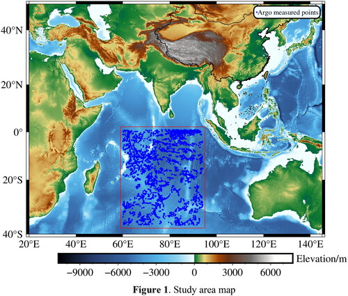
This article selects the central Indian Ocean (60°–95°E, 0°–37°S) as the study area (Figure 1). The main reason is that this area is far from land and can reduce the influence of radio frequency interference (RFI), which often causes significant errors. In addition, the temperature distribution in this region varies with latitude, with temperatures gradually decreasing south of the equator. The average temperature throughout the year is 15 °C–25 °C, and rainfall is most abundant near the equator (Lin et al. 2009). Thus, this area is the optimal region for studying the influence of various oceanic meteorological characteristics on SSS remote sensing inversion.

Figure 1. Study area map.

SMOS satellite data

The SMOS satellite, launched by the European Space Agency on November 2, 2009, is mainly used to detect and study global ocean salinity and soil moisture (Mecklenburg 2014). It carried a new type of radiometer called the two-dimensional aperture synthesis radiometer MIRAS (The Microwave Imaging Radiometer using Aperture Synthesis), which operates in the frequency band of 1,400–1,427 MHz and has a resolution of 30–90 km. The radiometer consists of 69 antenna-integrated receivers (LICEFs) capable of detecting the L-band of the Earth’s surface (He and Wu 2005; Jiang et al. 2000). In contrast to other satellites that measure salinity, the MIRAS radiometer carried by the SMOS satellite is not only sensitive to changes in soil moisture and seawater salinity, but also minimizes the influence of factors such as weather, atmosphere and vegetation cover on the results (Huang and Wu 2002).

This paper uses the SMOS Level 2 Marine salinity data product provided by the European Space Agency version 5.50. The SMOS L2 product data is provided on a 25 km resolution EASE 2 (Equal-Area Scalable Earth 2) grid for ascent and descent orbits, respectively. The sea surface salinity data is inferred from the brightness temperature (Tb) recorded by the MIRAS radiometer. Although all three SSS were inferred from the same maximum likelihood Bayes method using the first-order (L1) data, there were some differences in the geophysical model functions of the three SSS (Cao et al. 2019; Chen et al. 2018). Due to the larger errors in the descending orbit of the SMOS satellite compared to the ascending orbit and to avoid differences in data accuracy, this study selected daily data from 2019 consisting of ascending orbit data. The sea surface salinity (SSS) data was inverted using roughness model 3, which calculated empirical parameters based on a lot of data and imported parameters such as wind speed and temperature into the formula (Wang et al. 2013). The spatial resolution is 0.25° × 0.25°. SMOS-SSS, wind speed (WS), Tb_H(Horizontal Polarization Bright Temperature), Tb_V(Vertical Polarization Bright Temperature), sea surface temperature (SST), and Earth incidence angle (EIA) were all obtained from SMOS satellite data and can be downloaded from the European Space Agency (ESA) website (https://earth.esa.int/).

Argo data

Since its introduction in 1998, the global ocean temperature, salinity, and other measured data detected by Argo have been widely used (Balmaseda et al. 2007; Roemmich and Gilson 2019; Yang et al. 2016). Argo floats are neutral profile automatic drifting buoys that can automatically measure seawater temperature, salinity, and pressure between the sea surface and a depth of 2,000 meters in the ocean. The measured data is transmitted automatically to satellite ground receiving stations through satellite positioning and data transmission systems and is obtained as measured data after signal conversion and processing (Xu 2002). Due to the relationship between sea surface salinity and salinity values below the sea surface at a depth of 5 meters, Argo salinity data with depths between 0.5 meters and 5 meters can be used as sea surface salinity data. This data can be downloaded from the Argo website (http://www.Argo.org.cn/).

Meteorological factor data

This study’s meteorological factor data includes ECMWF Reanalysis v5(ERA5) and Climatic Research Unit gridded Time Series (CRU TS v4.05) data. ERA5 is the fifth-generation atmospheric reanalysis data for climate by the European Center for Medium-Range Weather Forecasts (ECMWF) (Chen et al. 2023; Jiang et al. 2021; Muñoz-Sabater et al. 2021). The gridded dataset has a spatial resolution of 0.1° × 0.1°, providing three climate factor data, which are total precipitation (RF), the 10-meter u-wind component (10 M-U), and the 10-meter v-wind component (10 M-V). CRU TS v4.05 is constructed from monthly observations at meteorological stations worldwide, excluding Antarctica, through interpolation by the Climatic Research Unit (CRU) (Zhou et al. 2023). It has a spatial resolution of 0.5° × 0.5° and provides four meteorological factor data, which are significant wave height (SWH), evaporation (EVA), wind direction (WR), and wave age (OMEGA). It should be noted that bathymetry can also have an effect on salinity. However, in this experiment, we only utilized salinity data at a depth of 5 meters, and therefore, we did not consider sea depth as an influencing factor.

Data preprocessing

Since the measured data of Argo are discrete point data, SMOS satellite provides grid data with a spatial resolution of 0.25° × 0.25°, and meteorological factors are data with different spatial resolutions, the three data formats are somewhat different. Before establishing the model, it is necessary to solve the problem of the three data’s different temporal and spatial resolutions. Spatio temporal matching of SMOS satellite data, meteorological factor data and Argo measured data is required. Referring to the data matching method proposed by Busalacchi et al. (2011), this paper adopts the matching principle that the spatial resolution is 0.25° × 0.25° grid and the temporal resolution is 12 h. SMOS satellite data, meteorological factor data and Argo measured data are matched in time and space. When the satellite SSS matched multiple Argo measured data in one day, Argo-SSS took the average value of the effective data within the range, and the final matching result obtained 2,980 effective data sets. To unify the dimensions of the input variables, 2,980 sets of data were obtained through spatiotemporal matching and normalized to a range of [0,1] to bring the numerical values of the effective data within this interval. The formula for calculating the normalized parameter value is: (1) $$x_{\mathit{\text{nr}}}=\frac{x-\mu }{\sigma }$$(1)

Where: $x$ is the original learning sample value, $\mu$ is the mean value of all learning samples, and $\sigma$ is the standard deviation of all learning samples.

The 2,980 normalized data were randomly divided into 2,086 training sets and 894 test sets according to a ratio of 7:3.

Research method

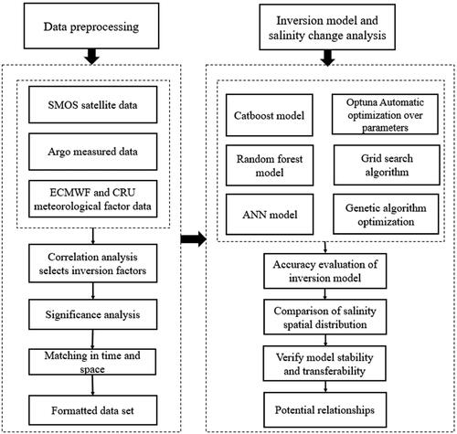
The specific steps for salinity inversion of the sea surface in this study are as follows: (1) Download the corresponding SMOS L2 satellite data and meteorological factor data based on the time information of measured sea surface salinity data. (2) Analyze the correlation between SSS and meteorological factor data, and select the most suitable meteorological factor data for salinity inversion. (3) Based on the temporal and spatial information of the measured data, merge SMOS satellite data and inversion factors to form a sample dataset. (4) Establish Optuna-Catboost, GA-ANN, and GS-RF salinity inversion models, and obtain the optimal inversion results by repeatedly searching and tuning parameters. (5) Select the best inversion algorithm based on evaluation indicators. (6) Analyze the salinity distribution characteristics of the model and compare them with the measured data of Argo. (7) Analyze the stability of the machine learning model by adding errors to the data, and verify the transferability of different models in different sea regions. (8) Analyze the importance of the 11 meteorological feature data for different models. (9) Analyze the potential relationship between salinity and meteorological characteristics. The experimental process is shown in Figure 2.

Figure 2. Technical roadmap.

Algorithm theory

Catboost algorithm

Catboost is a machine learning algorithm based on gradient lifting symmetric trees. Compared with the traditional GBDT algorithm, Catboost performs better in processing category features and missing values, supports CPU acceleration (Alshari et al. 2021), and efficiently trains models on large-scale data sets. In addition, Catboost also solves problems such as gradient bias and predicted migration, and uses a new gradient lifting mechanism to construct the model to reduce overfitting, which has fewer parameters and high accuracy and supports categorical variables (Yang and Yang 2022). Its powerful prediction performance and generalization ability can model and predict a large number of remote sensing and measured data. Due to its advantages of high performance, it has been widely used in processing category data.

The Catboost algorithm needs feature processing. In the input algorithm, its classification feature definition Equation (2)(2) $$x_k^i=\frac{{\sum }_{j=1}^{n}I\left\{x_j^i=x_k^i\right\}\cdot y_j+\beta \cdot \rho }{{\sum }_{j=1}^{n}I\left\{x_j^i=x_k^i\right\}+\beta }$$(2) is as follows: (2) $$x_k^i=\frac{{\sum }_{j=1}^{n}I\left\{x_j^i=x_k^i\right\}\cdot y_j+\beta \cdot \rho }{{\sum }_{j=1}^{n}I\left\{x_j^i=x_k^i\right\}+\beta }$$(2)

Where: $I$ is the index function, $x_j^i$ is the i − th subtype feature of the k − th training sample, $\rho$ is the added prior term, $\beta$ is the weight coefficient.

Artificial neural network algorithm

Artificial neural network (ANN) is an information processing and learning method based on the intelligent mechanism of the human brain. It usually consists of multiple neurons connected differently to form different networks (Jiao et al. 2016). Its characteristic is that it can learn implicit rules from large data and predict unknown data. It is commonly used in image processing, character recognition, prediction, and other aspects, with unique algorithmic advantages. Artificial neurons mainly have n independent variables, and the relationship between dependent variables and independent variables can be expressed by formulas (3) and (4). (3) $$S={\sum }_{i=1}^n{x}_i{w}_i+b$$(3) (4) $$y=f(S)$$(4)

Among them $x_i$ ($i=1,2,\dots ,n$) is the independent variable; $w_i$ ($i=1,2,\dots ,n$) is the weight of each independent variable; $b$ is the threshold value; $S$ Is the linear sum of the independent variable; $f$ is the activation function; $y$ is neuron output.

Random forest algorithm

Random Forest is an ensemble learning algorithm, a Bagging algorithm (Liu et al. 2012; Wang et al. 2011). Random forest is composed of strong decision trees with high depth. It can learn from multiple decision trees and determine the final prediction result by majority voting (Wang et al. 2021). Random forest algorithm is widely used in various fields because of its simple operation, high precision and strong anti-overfitting ability. The principle used by CART (Classification and Regression Tree) regression trees is the minimum mean square error (MSE), which means that for any split feature A and any split point s corresponding to it, the data sets D1 and D2 partitioned on both sides will be computed to find the feature and feature value split point that yields the minimum mean square error for each set, while also minimizing the sum of the mean square errors of D1 and D2. The expression is: (5) $$\mathrm{\text{min}}\left[\mathrm{\text{min}}\sum _{x_i\in D_1(A,s)}{(y_i-c_1)}^2+\mathrm{\text{min}}\sum _{x_i\in D_2(A,s)}{(y_i-c_2)}^2\right]$$(5)

Where:c₁ is the sample output mean of D₁ dataset, and c₂ is the sample output mean of D₂ dataset.

Parameter tuning

Optuna is an open-source hyperparameter optimization (HPO) framework. It determines combinations of hyperparameters by repeatedly calling the data and searches for hyperparameters in the regions with a higher possibility of the combinations. By repeating the search and continuously updating certain regions, it selects the optimal region and obtains the optimal hyperparameters (Zhang 2020).

Genetic algorithm (GA) is a reliable and efficient random search method in the field of deep learning. It realizes the optimization process of survival of the fittest through operation operations such as selection, crossover and mutation, and seeks the optimal solution with the maximum fitness in the population (Sang and Wook 1998; Lin et al. 2017).

Grid search algorithm (GS) arranges and combines all the values of parameters, lists all possible parameter combinations, and finally selects the parameter combination with the best performance through cyclic search (Wang et al. 2020). The grid search algorithm can obtain the optimal global solution within the specified range, but its defects are also obvious. When many parameters must be adjusted, the grid search will be time-consuming and inefficient (Guo et al. 2016).

To achieve the optimal inversion results for the Catboost, ANN, and RF models, this study used the Optuna hyperparameter automatic optimization method to optimize the Catboost model, the genetic algorithm (GA) to optimize the ANN model, and the grid search (GS) to optimize the RF model. Five parameters for each model were optimized, and 100 experiments were designed for each model to find the best performing hyperparameters through continuous searching, testing, and updating. Table 1 shows the optimal parameters obtained by the three models in 100 experiments.

Table 1. Parameter optimization results for the three models.

Optuna-Catboost		GA-ANN		GS-RF
Parameters	result	Parameters	results	Parameters	results
Depth	6	learning_rate	0.01	n_estimators	81
(6,10,1)		(0.01,0.03,0.05,0.07,0.09,0.1)		(1,101,10)
border_count	32	hidden_layer	2	max_depth	4
(1,254,1)		(1,5,1)		(4,8,1)
l2_leaf_reg	5	Nodes	5	min_samples_split	3
(5,8,1)		(1,10,1)		(2,5,1)
learning_rate	0.05	Optimizer	Adam	min_samples_leaf	2
(0.01,0.03,0.05,0.07,0.09,0.1)		(SGD、AdaGrad、Adam)		(1,3,1)
Iterations	1,000	Iterations	1,000	max_features	10
(800, 1,200, 100)		(800, 1,200,100)		(1,11,1)

Evaluation indicators

The experiment used the coefficient of determination (R²) and Mean absolute error in machine learning to compare and analyze the inversion accuracy of different algorithms. The best algorithm was analyzed for MAE (Mean Absolute Error) and RMSE. The coefficient of. determination evaluates an algorithm’s predictive ability and measures a model’s explanatory power (Huo et al. 2021; Peng et al. 2023). The three calculation formulas are as follows: (6) $$R^2=1-\frac{{\sum }_{i=1}^n{(y_i-{\widehat{y}}_i)}^2}{{\sum }_{i=1}^n{(y_i-{\overline{y}}_i)}^2}$$(6) (7) $$\mathit{\text{MAE}}=\frac{1}{n}{\sum }_{i=1}^n|y_i-{\widehat{y}}_i|$$(7) (8) $$\mathit{\text{RMSE}}=\sqrt{\frac{1}{n}{{\sum }_{i=1}^n(y_i-{\widehat{y}}_i)}^2}$$(8)

Pearson correlation coefficient analysis

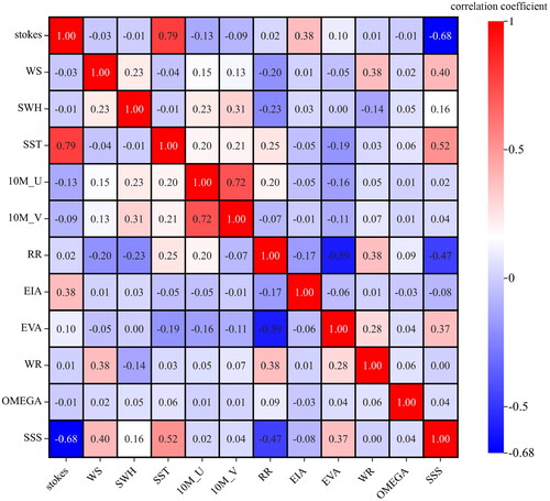
SSS inversion requires selecting inversion factors that are highly correlated with SSS as the learning samples for the model. In this paper, the Pearson correlation coefficient is used to measure the correlation between the inversion factor and the measured sea surface salinity data. The higher the correlation between the inversion factor and SSS, the better the inversion results. This study selected 11 meteorological data related to salinity inversion, namely: the first Stokes parameter (Tb_H + Tb_V), wind speed (WS), significant wave height (SWH), sea surface temperature (SST), meridional wind speed at 10 m height (10 M_U), zonal wind speed at 10 m height (10 M_V), rainfall (RR), Earth incidence angle (EIA), evaporation (EVA), wind direction (WR), and wave age (OMEGA). However, as too many input parameters can increase the model training time, the sensitivity of the 11 meteorological data to SSS changes was determined by calculating the Pearson correlation coefficient, as shown in Figure 3. Figure 3 shows that Stokes, RR, and EIA are negatively correlated with SSS, while other meteorological data are positively correlated with SSS. Compared with other meteorological data, Stokes, WS, SST, RR, and EVA correlate more significantly with SSS. Among them, the correlation coefficient between Stokes and SSS is the highest at 0.68.

Figure 3. Correlation analysis between SSS and meteorological data.

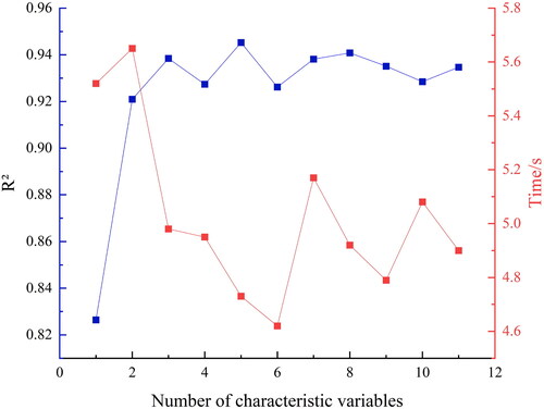
Figure 4 shows the number of input features in relation to R² and time. As the number of input features increases (the input rule is in order from highest to lowest), the R² fluctuates upward, and the time difference is not significant or even negligible. When the number of input features is 5, R² is the highest. Therefore, the most important five meteorological data, Stokes, WS, SST, RR, and EVA, were selected as the inversion factor input for the model, and the remaining meteorological factor data were eliminated from the matching dataset.

Figure 4. The relationship between the number of features entered and R²/time.

Feature importance analysis

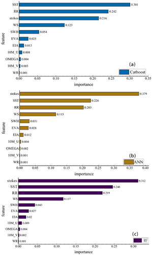
Due to the different importance of various meteorological factors in the inversion model of sea surface salinity in the central Indian Ocean, to explore the weights of different inversion factors in the model training and more effectively adjust the regression fit of the inversion factors to the actual measured salinity values of Argo, achieving the highest accuracy in the model inversion results. This paper is based on three ensemble learning algorithms in Sklearn: Catboost, ANN, and RF. Under the condition of keeping the default parameters unchanged, the importance of 11 meteorological feature factors on the inversion of sea surface salinity is calculated for each model, and the results are analyzed with three significant figures reserved. The higher the importance of the result, the higher the contribution of the meteorological factor variable to the inversion of sea surface salinity. Figure 5 shows the importance analysis diagram of meteorological features of three machine learning models. The top five meteorological factors regarding feature importance are SST, stokes, WS, RR, and SWH, due to the obvious tropical oceanic and monsoon climate in the Indian Ocean, the horizontal brightness temperature and vertical brightness temperature are greatly affected by the seasonal wind vector. Combined with the feature correlation (Figure 3), it was found that SST is the meteorological factor with the highest contribution in the Catboost model, but its correlation with SSS is not the highest, while in the ANN and RF models, stokes is the meteorological factor with the highest importance, indicating that the importance of the same meteorological feature factor is different for different models. In addition, compared with SWH, EVA has a higher correlation with SSS. Choosing EVA as the independent variable in the model and inputting it into the inversion model, the contribution of SWH, which was not selected as an inversion factor, to the model inversion is higher than that of EVA. This may be because the effective wave height in the Indian Ocean in 2019 was higher due to the influence of the southeast monsoon or tsunami.

Figure 5. Significance analysis of meteorological features.

Result analysis and discussion

Accuracy evaluation

To select the optimal algorithm for salinity inversion and improve the accuracy of SMOS satellite product data, this study used evaluation indicators and scatter plots to analyze the model’s inversion ability and the predicted values’ deviation degree. Table 2 shows the results of evaluation indicators of the training set and test set. Through analysis, it is found that RMSE and MAE of salinity of SMOS satellite are 0.7967 psu and 0.5635 psu, respectively. The R², RMSE and MAE of salinity inversion between the Catboost model training set based on Optuna super parameter automatic optimization and Argo measured salinity data are as high as 0.9813, 0.2147 psu and 0.1803 psu. The R² of salinity inversion between the Optuna-Catboost test set and Argo-SSS is 0.9452, RMSE is 0.2360 psu, and RMSE is 0.1816 psu. Although the accuracy of the test set is slightly lower than that of the training set, its accuracy is still significantly better than that of SMOS L2 product salinity data.Moreover, the regression effect is better than GA-ANN and GS-RF models, indicating that the Catboost model is suitable for salinity inversion, indicating that the model can effectively solve the problem of gradient deviation and prediction deviation to reduce the occurrence of overfitting； The test set accuracy of GA-ANN and GS-RF is also lower than that of the training set. The RMSE of the test set are 0.3004 psu and 0.3156 psu respectively, and MAE are 0.2486 psu and 0.2641 psu respectively. The inversion results of SSS are also better than those of SMOS satellite salinity. In conclusion, the inversion results of the three models established in this paper all have higher accuracy than those of the salinity products of the SMOS satellite, among which the Optuna-Cat boost model has the best effect of salinity inversion.

Table 2. Evaluation indicators results of the training set and test set.

models	Indicators
		R^2	RMSE	MAE
training set	Optuna-Catboost	0.9813	0.2147	0.1748
	GA-ANN	0.9490	0.2480	0.2990
	GS-RF	0.9335	0.2685	0.3211
test set	Optuna-Catboost	0.9452	0.2360	0.1816
	GA-ANN	0.9123	0.3004	0.2486
	GS-RF	0.9018	0.3156	0.2641
SMOS L2		0.7424	0.7967	0.5635

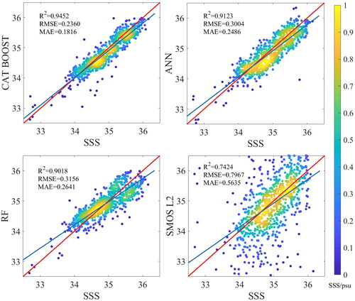
Figure 6 are scatter plots of the linear regression between the measured Argo salinity data on the test set and the predicted salinity values of the Optuna-Catboost, GA-ANN, and GS-RF models, as well as the SMOS L2 salinity product data. Based on the distribution of scatter plots and the fitted line, it can be seen that the Optuna-Catboost model has a good fitting degree with the measured Argo salinity data. The predicted result of this model is randomly distributed on both sides of the 1:1 line, especially in the 35–36 psu interval, where the fitted line of the scattered points is closer to the 1:1 line. However, the predicted result is relatively poor between 34 and 35 psu, smaller than the measured salinity. Overall, the error fluctuation between the salinity retrieved by the Optuna-Catboost model and the measured salinity is the smallest. This is related to the robust loss function of the Catboost model, which makes it strong against abnormal data and has a strong anti-interference ability. The results of the GA-ANN model show a relatively uniform distribution in the range of 34–36 psu, with almost no anomalous situations occurring. However, the predicted salinity values are poor in low salinity conditions, with the estimated salinity values varying greatly. This demonstrates that the GA-ANN model is particularly effective in inverting salinity in high salinity regions. The salinity inversion results of the GS-RF model are good in the predicted range of 34–35 psu, but as the salinity increases, the error with the measured salinity from Argo gradually increases, with an RMSE of 0.3156 psu. The fitting effect of SMOS L2 salinity data with Argo measured salinity is poor, with a scattered distribution and a coefficient of determination R² of only 0.7424, significantly lower than the salinity inversion results of the three machine learning models.

Figure 6. Scatter plots of inversion model.

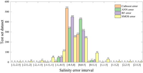
In addition, this study also analyzed the absolute error distribution of the Optuna-Cat boost model, the GA-ANN model, the GS-RF model, SMOS-SSS and Argo-SSS in the test set. The results are shown in Figure 7. The absolute errors of the three models for salinity, SMOS-SSS and Argo-SSS are mainly distributed between [−0.5, 0.5], with 810, 762, and 761 data points in their respective ranges, accounting for 97.8%, 92.0%, and 91.9% of the total test set. In contrast, SMOS-SSS only has 491 data points in the [−0.5, 0.5] range, accounting for only 59.3% of the total test set. In addition, the salinity values predicted by the three models are all within the interval [−1.5,1], while SMOS-SSS is distributed within the error interval [−3.5,3.5]. In comparison, the error value of SMOS-SSS is larger. In summary, the three algorithms used in this paper to invert salinity are significantly better in quality than the SMOS L2 product data. Among them, the Optuna-Catboost model has better accuracy and stability in inverting salinity, indicating the potential of Catboost in salinity remote sensing inversion.

Figure 7. Histogram of the error between the salinity inverted by the model and the salinity measured by Argo.

The spatial distribution and comparison of salinity

Referring to Liu et al. (2022), the Kriging interpolation method with linear unbiased optimal estimation was used to analyze the spatial distribution of salinity. In this paper, salinity data retrieved from the SMOS L2 satellite, Argo measurement data, and Optuna-Catboost, GA-ANN and GS-RF models were analyzed in the central Indian Ocean (60°–95°E, 0°–37°S) for optimal interpolation. The spatial distribution characteristics of the three types of SSS data were analyzed and compared (refer to Figure 8). According to the spatial distribution of salinity measured by Argo, it can be found that the salinity trend in the central Indian Ocean is lower in the north and higher in the south. The salinity values are lower at (83°–88°E, 24°–27°S) and (68°–72°E, 17°–20°S), with the lowest value of 32.043 psu; and higher at 30°–35°S, with the highest value of 36.344 psu. In addition, near the equator, salinities between 60°E and 80°E are higher than those between 80°E and 95°E. This is because the area between 60°E–80°E is close to the Arabian Sea, which is greatly affected by the dry and hot airflow from the land, and the water temperature can reach above 30 °C. The salinity is generally less than 35psu in the rainy season and greater than 36psu in the dry season. The salinity data measured by Argo and the salinity data inverted by the models roughly show the same trend, but there is a certain deviation in the salinity values in some local areas.

Figure 8. Spatial distribution of salinity of Argo, Catboost, ANN, RF and SMOS.

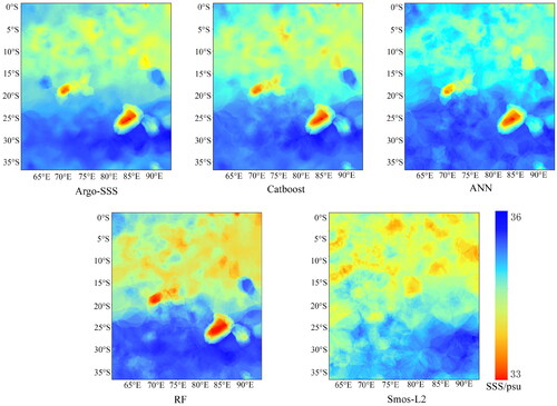
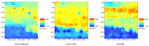
While 80°E∼95°E is close to the Bay of Bengal where the salinity of the tropical sea surface is the lowest, there is a large amount of rainfall in this sea area and the inflow of poor fresh water from the surrounding runoff will cause the sea surface stratification and the increase of the sea surface roughness, which will lead to the decrease of the inversion salinity value. The difference in salinity between the eastern and western coasts of the tropical Indian Ocean is mainly due to the difference in freshwater flux. The salinity distribution of the Catboost model inversion, ANN model and RF model was compared with Argo measured salinity distribution. It was found that the salinity values of the three models also showed a trend of low in the north and high in the south. Although there were various deviations, their errors were all within the allowed accuracy range. The spatial distribution of salinity retrieved by the Catboost model is the most similar to that measured by Argo. The salinity value in the range of 0°S–20°S is slightly lower than that measured by Argo. This phenomenon is related to the high probability of salinity being affected by environmental factors due to its location in the offshore sea. By comparing the spatial distribution of salinity between the SMOS satellite and Argo measurement, it is found that: Although the salinity distribution of SMOS satellite is also low in the north and high in the south, the salinity in the whole study area is significantly lower than that measured by Argo, showing a low coincidence. In particular, the salinity values in the 0°S–20°S region are all about 33.5 psu, and the salinity values measured by Argo are about 34.5 psu, with an error close to 1.

Figure 9 shows the error plots of predicted salinity values from the Optuna-Cat boost model, the GA-ANN model, and the GS-RF model compared to the measured salinity values from Argo. Combined with the results in Figure 8, it can be observed that the salinity images inverted using the Optuna-Catboost model have a high spatial consistency with the true salinity images, with salinity errors ranging from −0.57 to 0.46 psu. The results are particularly good in the lower salinity regions (i.e., blue-green regions), with errors almost approaching zero. However, in higher salinity regions (25°S–37°S), the inverted salinity values are generally lower than measured. This phenomenon may be due to the fact that the westerlies prevail near 30°S in the Indian Ocean, and the average temperature decreases significantly toward the south throughout the year, while also being affected by the counterclockwise circulation of the southern Indian Ocean’s oceanic currents. For the GA-ANN model, the salinity error is between −0.81 and 0.65psu, and ANN-SSS is slightly higher than Argo-SSS in most areas, among which, ANN-SSS is about 0.5psu higher than Argo-SSS in the 15°S–25°S area, because the southeast trade winds blow in this area. The northeast monsoon and southeast trade winds meet near the equator, forming an intense and rainy intertropical convergence zone, resulting in low measured salinity values in Argo. Compared with Optuna-Catboost and GA-ANN models, the error of the GS-RF model is larger, ranging from −1.31 to 0.86psu, and RF-SSS is significantly higher than Argo-SSS in the area of 5°S–10°S. The main reason is that this sea area is located near the equator and the annual average temperature is 28 °C. Even some areas of the sea are as high as 30 °C, called tropical oceans.

Figure 9. Salinity residual distribution of Catboost, ANN, RF and Argo.

Model stability evaluation

Additionally, this article used data from January to March 2020 as independent validation data to evaluate the performance of the models. After preprocessing the validation data, 716 sets of data were put into the optimal Optuna-Catboost model, GA-ANN and GS-RF model, and three inversion results of 2020-Catboost, 2020-ANN and 2020-RF were obtained, respectively. It was found that the Optuna-Catboost model had a correlation coefficient R² of 0.9551, RMSE of 0.2296 psu, and MAE of 0.1791 psu when predicting the salinity from January to March 2020, which validates the model’s feasibility.

To make the experiment more persuasive, Wen et al. (2000) proposed the method of adding random interference errors of different magnitudes to the data artificially. Random errors of 1%, 2%, and 5% were added to the sample data respectively, and the three machine learning models were inputted to obtain salinity inversion results with different random errors while controlling the same input model training set. The stability of the three inversion models was verified by comparing evaluation indicators. Figure 10 and Table 3 shows the evaluation results of the model with added random errors. It was found that the results with added random errors showed a gradual decrease in R², but the decrease was relatively small, indicating that the model was relatively stable. In contrast, the RMSE gradually increased with added random errors, and the magnitude of the increase also gradually increased. The MAE showed a distribution trend of first increasing, then decreasing, and then increasing again, with a more obvious increase and decrease than R² and RMSE. This may be due to the parameter adjustment results of the Catboost model. The GA-ANN model had a larger jump in salinity inversion results after adding 1%, 2%, and 5% random errors compared to the Optuna-Catboost model and GS-RF model, especially in terms of RMSE, which may be related to the fewer hidden layers in the inversion model. The GS-RF model had the best stability among the three models. After adding random errors, the change in R² was relatively flat, and both RMSE and MAE showed a gradually increasing trend, but there were no significant jumps, indicating that the tree structure of the model could support its stability well. Overall, the three evaluation indicators did not show a significant increase or decrease and were within an acceptable range of error, indicating that using the Optuna-Catboost model, GA-ANN model, and GS-RF model to invert salinity has a certain degree of stability.

Figure 10. R² of the random error model.

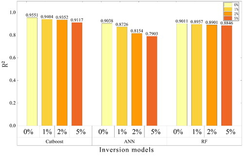
Table 3. RMSE and MAE of the random error model.

		2020	1%	2%	5%
Catboost	RMSE/psu	0.2296	0.2310	0.2463	0.2607
	MAE/psu	0.1791	0.1968	0.1824	0.2093
ANN	RMSE/psu	0.2109	0.2065	0.2291	0.2680
	MAE/psu	0.2005	0.2161	0.2183	0.2408
RF	RMSE/psu	0.2044	0.2076	0.2153	0.2203
	MAE/psu	0.1951	0.2071	0.2179	0.2203

Model transferability verification

Referring to the method of Ai et al. (2019), The 90 sets of buoys in the South China Sea are used to verify the applicability of the model in other sea areas. The position of the buoy is shown in Table 4. To obtain the model sample dataset, the selected Argo buoy data is preprocessed by time and space matching and normalization with corresponding SMOS satellite data and meteorological data. Then, the processed data is brought into the optimal Optuna-Catboost, GA-ANN and GA-RF to obtain the inversion results. The actual salinity data in the South China Sea and the model predicted salinity are shown in Figure 11. From the result analysis, it can be found that the salinity result of the Optuna-Catboost model is more in line with the Argo buoy data in terms of fluctuations and amplitudes. The RMSE of the salinity inversion of this model is 0.2260 psu, and the mean absolute error is 0.1906 psu. The GA-ANN model has poor performance in testing model transferability. The result chart shows that the salinity inversion result of this model has a larger fluctuation amplitude compared with the Argo actual measurement data. From the perspective of absolute error analysis, the absolute errors within 0.5 psu account for 31.5% of the total sample data, the absolute errors within 1 psu and above 1 psu account for 47.2% and 21.3% of the total sample data, respectively. The poor performance of the GA-ANN model in transferability may be related to the small sample data. The RMSE of the salinity inversion of the GS-RF model is 0.2637 psu, and the mean absolute error is 0.2359 psu. The absolute errors of this model within 0.5 psu, 1 psu, and above 1 psu account for 68.4%, 29.1%, and 2.5% of the total sample data, respectively. Due to the stable tree structure of the RF model, it shows stable and observable effects in salinity inversion in different seas.

Figure 11. Salinity inversion results of machine learning in the south China Sea.

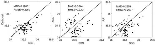
Table 4. The measured buoy site in South China sea.

Number	Longitude(°E)	Latitude(°N)
1	111.927	20.368
2	112.128	19.871
3	113.442	21.554
4	114.419	19.609
5	115.598	20.863
6	116.506	21.082
7	117.040	21.577

Potential relationships between meteorological characteristics and salinity changes

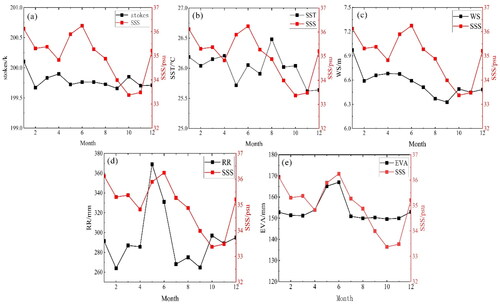
This paper examines the potential relationships between five meteorological features and salinity, as depicted in Figure 12. The central Indian Ocean resides within the equatorial low-pressure area, featuring elevated sea surface temperatures due to reduced wind speeds and the ascent of warm, humid air, which leads to precipitation (Athira et al. 2023). Figure 12b illustrates that monthly sea surface temperature (SST) is influenced by climate factors, with the Indian Ocean’s circulation cold current in November and December contributing to decreased water temperatures in this region. November records the lowest temperature at 25.62 °C, while August, benefiting from solar radiation as the primary heat source, registers the highest temperature at 26.51 °C. The annual average for this area is 26.01 °C. The SST and salinity (SSS) trends indicate that SSS variations in January–April are significantly impacted by SST, while during May-August, salinity levels may be greatly influenced by rainfall. Figure 12c demonstrates the formation of a distinct North Indian Ocean monsoon circulation in the Indian Ocean due to the influence of the South Asian tropical monsoon climate. In January, the Northeast monsoon prevails, creating a counterclockwise circulation with a maximum wind speed of 6.97 m, while in September, under the influence of the southwest monsoon, the wind speed reaches its minimum at 6.33 m. Figure 12d shows that the maximum monthly precipitation occurs in May at 369 mm, whereas the minimum is recorded in February at 264 mm. With the exception of May and June, seasonal variations in precipitation are relatively small, leading to an annual average of 293.1 mm. The trends in rainfall (RR) and SSS indicate that changes in SSS during May–June and October are significantly influenced by RR.

Figure 12. Potential relationships between meteorological characteristics and salinity changes.

Conclusion

This article compares three machine learning salinity inversion models based on the central Indian Ocean (60°–95°E, 0°–37°S). Firstly, using the Pearson correlation coefficient, the meteorological characteristics are determined for the inversion model to reduce training time and data redundancy. The selected five meteorological characteristics: the first Stokes parameter (Tb_H + Tb_V), sea surface temperature (SST), wind speed (WS), precipitation (RR), and evaporation (EVA) are matched with SMOS-SSS and Argo-SSS temporally and spatially. Secondly, Optuna-Cat boost, GA-ANN, and GS-RF models are established to predict salinity values. Based on the evaluation indicators, the model most suitable for salinity inversion in the study area is selected, and the relationship between salinity variation and climatic and meteorological characteristics is also analyzed. Finally, independent data sets are used to verify the stability and transferability of the three machine learning models, and the importance of meteorological characteristics to the three inversion models is analyzed.

The experimental results show that the regression fitting R² of the three machine learning retrieval models with Argo measured data are 0.9452, 0.9123 and 0.9018, the corresponding RMSE values are 0.2360 psu, 0.3004 psu, and 0.3156 psu, and the MAE values are 0.1816 psu, 0.2486 psu, and 0.2641 psu, respectively. In terms of the fitting degree, the Optuna-Catboost model has the best effect on estimating the salinity of the central Indian Ocean. Comparing the spatial distribution of the SSS retrieval of the three machine learning models with the spatial distribution of Argo-SSS, salinity trends generally from north to south, exhibiting a high degree of consistency. Independent data sets from different years were applied to the machine learning models, and errors were introduced into the data to verify the stability of the models. The transferability of the models was analyzed by conducting salinity inversions in different marine areas. The high-precision inversion results demonstrate the feasibility of using the three machine learning models for SSS inversion and provide data support for related research disciplines. Sea surface salinity is an important feature of oceanography, and salinity inversion is an extremely difficult problem. Many aspects of the experiment still need to be improved, such as selecting different inversion factors and using different machine learning models for salinity inversion. Increasing the amount of data can also improve the accuracy of inversion. These issues all require further in-depth research.

Acknowledgments

The authors would like to thank the European Centre for Medium-Range Weather Forecasts (ECMWF), data from the SMOS satellite and the Argo observations, which were instrumental to the success of this research. The authors are also grateful to Yuan Huang from Singularity Innovation Inc and Jingran Sheng from Ningbo Globfishing Corp for their significant contributions to the revision of this manuscript.

Disclosure statement

No conflict of interest was reported by the author (s).

Additional information

Funding

This research was funded by the Natural Science Foundation of Guangxi Province (CN) (2022GXNSFBA035637), and the ‘Ba Gui Scholars’ program of the provincial government of Guangxi.

References

- Ai, B., Wen, Z., Jiang, Y., Gao, S., and Lv, G.N. 2019. “Sea surface temperature inversion model for infrared remote sensing images based on deep neural network.” Infrared Physics & Technology, Vol. 99: pp. 231–239. doi:10.1016/j.infrared.2019.04.022.
- Alshari, H., Saleh, A.Y., and Odabaş, A. 2021. “Comparison of gradient boosting decision tree algorithms for CPU performance.” Journal of Institue of Science and Technology, Vol. 37 (No. 1): pp. 157–168.
- Alvera-Azcárate, A., Barth, A., Parard, G., and Beckers, J.-M. 2016. “Analysis of SMOS sea surface salinity data using DINEOF.” Remote Sensing of Environment, Vol. 180: pp. 137–145. doi:10.1016/j.rse.2016.02.044.
- Athira, U.N., Abhilash, S., and Sabeerali, C.T. 2023. “Paradigm shift in the onset phase of the Indian Summer Monsoon since 2000 and its potential connection to South Indian Ocean.” Atmospheric Research, Vol. 296: pp. 107050. doi:10.1016/j.atmosres.2023.107050.
- Bai, Y., Zhao, T. j., Jia, L., Cosh, M.H., Shi, J.C., Peng, Z.Q., Li, X.J., and Wigneron, J.P. 2022. “A multi-temporal and multi-angular approach for systematically retrieving soil moisture and vegetation optical depth from SMOS data.” Remote Sensing of Environment, Vol. 280: pp. 113190. doi:10.1016/j.rse.2022.113190.
- Balmaseda, M., Anderson, D., and Vidard, A. 2007. “Impact of Argo on analyses of the global ocean.” Geophysical Research Letters, Vol. 34 (No. 16): pp. L16605. doi:10.1029/2007GL030452.
- Bao, S.L., Zhang, R., Wang, H.Z., Yan, H.Q., Chen, J., and Wang, Y.J. 2023. “Correction of satellite sea surface salinity products using ensemble learning method.” IEEE Access., Vol. 11: pp. 17870–17881. doi:10.1109/ACCESS.2021.3057886.
- Busalacchi, A.J., Hackert, E.C., Alory, G., Arkin, P.A., Ballabrera, J., Delcroix, T.C., Janowiak, J., Ren, L., Murtugudde, R.G., and Zhang, R. 2011. “Spatio-temporal variability and error structure of SSS in the tropics.” Fall Meeting Abstracts, Vol. 1: pp. 1627.
- Cao, K.X., Sun, W.F., Meng, J.M., and Zhang, J. 2019. “Assessment and comparison of sea surface salinity data derived from SMAP and SMOS based on Argo measurements.” Advances in Marinee Science, Vol. 37 (No. 4): pp. 574–587.
- Chen, J.Z., Shi, X.H., and Wen, M. 2023. “Applicability of ERA5 surface wind speed data in the region of “two oceans and one sea.” Meteor Mon, Vol. 49 (No. 1): pp. 39–51. doi:10.7519/j.issn.1000-0526.2022.072301.
- Chen, Z. w., Li, Q.X., and Li, Y. 2018. “Comparison and analysis of sea surface salinity measurement method and data between SMOS and aquarius.” Aerospace Shanghai, Vol. 35 (No. 2): pp. 37–48. doi:10.19328/j.cnki.1006-1630.2018.02.005.
- Furue, R., Takatama, K., Sasaki, H., Schneider, N., Nonaka, M., and Taguchi, B. 2018. “Impacts of sea-surface salinity in an eddy-resolving semi-global OGCM.” Ocean Modelling, Vol. 122: pp. 36–56. doi:10.1016/j.ocemod.2017.11.004.
- Gao, M., Huang, X.Y., Wang, F., Zhang, H.L., Zhao, H.X., and Gao, X.Y. 2022. “Sea surface salinity inversion based on DNN model.” Advances in Marine Science, Vol. 40 (No. 3): pp. 496–504. doi:10.12362/j.issn.1671-6647.20210409001.
- Guo, F.H., Zhang, C.M., and Jiao, W.J. 2016. “Research progress on mesh parameterization.” Ruan Jian Xue Bao/Journal of Software, Vol. 27 (No. 1): pp. 112–135. doi:10.13328/j.cnki.jos.004919.
- He, B.Y., and Wu, J. 2005. “Optimization on circular thinned array for two-dimensional synthetic aperture microwave radiometer.” Acta Electronica Sinica, Vol. 33 (No. 9): pp. 1607.
- Huang, Y., and Wu, J. 2002. “Study on image theory of high resolution two-dimensional synthetic aperture microwave radiometer.” Acta Electonica Sinica, Vol. 30 (No. 5): pp. 697.
- Huo, C.G., Huo, F.F., and Dong, K. 2021. “Scientific topic prediction | The popularity prediction of scientific topics based on LSTM.” Library and Information Knowledge, Vol. 38 (No. 2): pp. 25–34. doi:10.13366/j.dik.2021.02.025.
- Jang, E., Kim, Y.J., Im, J., Park, Y.G., and Sung, T. 2022. “Global sea surface salinity via the synergistic use of SMAP satellite and HYCOM data based on machine learning.” Remote Sensing of Environment, Vol. 273: pp. 112980. doi:10.1016/j.rse.2022.112980.
- Jiang, J.S., Zhang, Y. H., and Dong, X.L. 2000. “The discussion of up to date technologies in microwave remote sensing and the new generation of space remote sensing method.” Engineering Science, Vol. 08: pp. 76–82.
- Jiang, Q., Li, W., Fan, Z., He, X., Sun, W., Chen, S., Wen, J., Gao, J., and Wang, J. 2021. “Evaluation of the ERA5 reanalysis precipitation dataset over Chinese Mainland.” Journal of Hydrology, Vol. 595: pp. 125660. doi:10.1016/j.jhydrol.2020.125660.
- Jiao, L.C., Yang, S.Y., Liu, F., Wang, S.G., and Feng, Z.X. 2016. “Seventy years beyond neural networks: Retrospect and prospect.” Chinese Journal of Computers, Vol. 39 (No. 8): pp. 1697–1716. doi:10.11897/SP.J.1016.2016.01697.
- Li, C.J., Zhao, Q.H., and Zhao, H. 2018. “Retrieve salinity using BP Neural Networks model based on SMOS data.” Periodical of Ocean University of China, Vol. 13 (No. 1): pp. 125–134. doi:10.16441/j.cnki.hdxb.20150261.
- Lin, A.L., Li, T., and Fu, Xh. 2009. “Impact of air-sea interactions over the Indian Ocean on the climatological state of tropical atmospheric circulation in boreal summer.” Chinese Journal of Atmospheric Sciences, Vol. 33 (No. 6): pp. 1123–1136.
- Lin, Y., Zhao, H., and Ding, H. 2017. “Solution of inverse kinematics for general robot manipulators based on multiple population genetic algorithm.” Journal of Mechanical Engineering, Vol. 53 (No. 3): pp. 1–8. doi:10.3901/JME.2017.03.001.
- Liu, Q.Q., Zhang, Y.S., Xu, M., Li, H.P., and Liu, H.X. 2022. “SMAP satellite sea surface inversion model based on machine learning.” Advance in Marine Science, Vol. 40 (No. 1): pp. 56–65.
- Liu, T.S., Zheng, M.P., and Guo, Z.T. 1998. “Initiation and evolution of the asian monsoon system timely coupled with the ice-sheet growth and the tectonic movements in Asia.” Quaternary, Vol. 3 (No. 194): pp. 3.
- Liu, Y., Wang, Y., and Zhang, J. 2012. “New machine learning algorithm: Random forest.” Information Computing and Applications: Third International Conference, ICICA 2012, Chengde, China, September 14-16, Proceedings 3. Berlin Heidelberg: Springer. pp. 246–252. doi:10.1007/978-3-642-34062-8_32.
- Ma, W.T., Du, Y.L., Liu, G.H., Yu, Y., Yang, X.F., Yang, J., and Chen, K.S. 2021. “Study on direction dependence of the fully polarimetric wind-induced ocean emissivity at L-band using a semi-theoretical approach for Aquarius and SMAP observations.” Remote Sensing of Environment, Vol. 265: pp. 112661. doi:10.1016/j.rse.2021.112661.
- Mecklenburg, S. 2014. “ESA's Soil Moisture and Ocean Salinity Mission-An overview on the mission’s performance and scientific results.” EGU General Assembly Conference Abstracts.
- Muñoz-Sabater, J., Dutra, E., Agustí-Panareda, A., Albergel, C., Arduini, G., Balsamo, G., Boussetta, S., et al. 2021. “ERA5-Land: A state-of-the-art global reanalysis dataset for land applications.” Earth System Science Data, Vol. 13 (No. 9): pp. 4349–4383. doi:10.5194/essd-13-4349-2021.
- Olmedo, E., Martínez, J., Turiel, A., Ballabrera-Poy, J., and Portabella, M. 2017. “Debiased non-Bayesian retrieval: A novel approach to SMOS Sea Surface Salinity.” Remote Sensing of Environment, Vol. 193: pp. 103–126. doi:10.1016/j.rse.2017.02.023.
- Peng, T., Zhao, L., Zhang, A.J., Yang, X.N., Zhou, Z., and Chang, X.H. 2023. “UAV hyperspectral response characteristics and estimation model construction of soil total nitrogen.” Transactions of the Chinese Society of Agricultural Engineering, Vol. 39 (No. No. 4): pp. 92–101. doi:10.11975/j.issn.1002-6819.202211021.
- Reul, N., Grodsky, S.A., Arias, M., Boutin, J., Catany, R., Chapron, B., D'Amico, F., et al. 2020. “Sea surface salinity estimates from spaceborne L-band radiometers: An overview of the first decade of observation (2010–2019).” Remote Sensing of Environment, Vol. 242: pp. 111769. doi:10.1016/j.rse.2020.111769.
- Roemmich, D., and Gilson, J. 2019. “The 2004–2008 mean and annual cycle of temperature, salinity, and steric height in the global ocean from the Argo Program.” Progress in Oceanography, Vol. 82 (No. 2): pp. 81–100. doi:10.1016/j.pocean.2009.03.004.
- Sang, Y.M., and Wook, H.K. 1998. “Genetic-based fuzzy control for half car active suspension systems.” International Journal of Systems Science, Vol. 29 (No. 7): pp. 699–710. doi:10.1080/00207729808929564.
- Scotese, C.R., Boucot, A.J., and McKerrow, W.S. 1999. “Gondwanan palaeogeography and pal˦ oclimatology.” Journal of African Earth Sciences, Vol. 28 (No. 1): pp. 99–114. Vol(NO doi:10.1016/S0899-5362(98)00084-0.
- Tangdamrongsub, N., Han, S.C., Yeo, I.Y., Dong, J.Z., Steele-Dunne, S.C., Willgoose, G., and Walker, J.P. 2020. “Multivariate data assimilation of GRACE, SMOS, SMAP measurements for improved regional soil moisture and groundwater storage estimates.” Advances in Water Resources, Vol. 135 pp. 103477. doi:10.1016/j.advwatres.2019.103477.
- Tian, T., Cheng, L.J., Wang, G.J., Abraham, J., Wei, W.X., Ren, S.H., Zhu, J., Song, J.Q., and Leng, H.Z. 2022. “Reconstructing ocean subsurface salinity at high resolution using a machine learning approach.” Earth System Science Data, Vol. 14 (No. 11): pp. 5037–5060. doi:10.5194/essd-14-5037-2022.
- Wang, A.P., Wan, G.W., Cheng, Z.Q., and Li, S.K. 2011. “Incremental learning extremely random forest classifier for online learning.” Journal of Software, Vol. 22 (No. 9): pp. 2059–2074. doi:10.3724/sp.j.1001.2011.03827.
- Wang, H., Jiang, Y.N., Zhang, X., Zhong, H.R., Chen, Q.X., and Gao, S.C. 2021. “Lithology identification method based on gradient boosting algorithm.” Journal of Jilin University, Vol. 51 (No. 3): pp. 940–950. doi:10.13278/j.cnki.jjuese.20200081.
- Wang, H., Yan, J.Y., Fu, G.M., and Wang, X. 2020. “Current status and application prospect of deep learning in geophysics.” Progress in Geophysics, Vol. 35 (No. No. 2): pp. 0642–0655. doi:10.6038/pg2020CC0476.
- Wang, X.X., Wang, X., Han, Z., and Yang, J.H. 2015. “Radio frequency interference detection and characteristic analysis based on the l band stokes parameters remote sensing data.” Journal of Electronics & Information Technology, Vol. 37 (No. 10): pp. 2342–2348. doi:10.11999/JEIT141577.
- Wang, X.X., Yang, J.H., Zhao, D.Z., Wang, X., and Sun, G.L. 2013. “SMOS satellite salinity data accuracy assessment in the China coastal areas.” Acta Oceanologica Sinica, Vol. 35 (No. 5): pp. 169–176. doi:10.3969/j.issn.0253-4193.2013.05.019.
- Wen, Y.B., Wan, Y.Y., Hu, J.F., Fu, Z.W., Duan, Y.K., and Hu, Y.L. 2000. “The effection of sampling precision on imaging in cross-hole tomography.” Journal of Yunnan University, Vol. 22 (No. S1): pp. 49–53.
- Wu, F.F., Fu, Z.Y., Hu, L.S., Zhang, F., Du, Z.H., and Liu, R.Y. 2021. “Retrieval of sea surface salinity in the Gulf of Mexico based on random forest method.” Haiyang Xuebao, Vol. 43 (No. 9): pp. 126–136. doi:10.12284/hyxb2021146.
- Xu, J. P. 2002. Argo Global Ocean Observation Exploration. Beijing: China Ocean Press.
- Yang, S.L., Zhou, S.F., Zhou, W.F., Wu, Y.M., and Zhang, B.B. 2016. “The relationship between skipjack Katsuwonus pelam is catch and water temperature and surface salinity in the west-central Pacific Ocean based on Argo data.” Journal of Dalian Fisheries University, Vol. 25 (No. 1): pp. 34–40. doi:10.3969/j.issn.1000-9957.2010.01.007.
- Yang, T., and Niu, G.S. 2021. “Seasonal and interannual variation characteristics of the tropical Indian ocean’s intertropical convergence zone.” Climate Change Research Letters, Vol. 10 (No. 06): pp. 584–597. doi:10.1007/s00382-020-05195-5.
- Yang, X.J., and Yang, X.H. 2022. “Reflections on the application of machine learning in the development of medical data.” Advances in Applied Mathematics, Vol. 11: pp. 3496. doi:10.12677/aam.2022.116372.
- Zhang, L.J., Zhang, Y.F., and Yin, X.B. 2023. “Aquarius sea surface salinity retrieval in coastal regions based on deep neural networks.” Remote Sensing of Environment, Vol. 284: pp. 113357. doi:10.1016/j.rse.2022.113357.
- Zhang, Y. 2020. Research on Hyperparameter Optimization for Deep Learning models. Beijing: Capital University of Economics and Business. doi:10.27338/d.cnki.gsjmu.2020.000828.
- Zhao, H., and Wang, C.J. 2016. “Study on the sea surface salinity model based on SMOS data.” Journal of Ocean Technology, Vol. 35 (No. 01): pp. 15–22. doi:10.3969/j.issn.1003-2029.2016.01.002.
- Zhao, W.J., Li, H.P., and Liu, H.X. 2022. “Remote sensing retrieval of sea surface salinity based on RBF neural network from SMAP satellite.” Advances in Marine Science, Vol. 40 (No. 3): pp. 513–522. doi:10.12362/j.issn.1671-6647.20210702001.
- Zhou, S., Yu, B., and Zhang, Y. 2023. “Global concurrent climate extremes exacerbated by anthropogenic climate change.” Science Advances, Vol. 9 (No. 10): pp. eabo1638. doi:10.1126/sciadv.abo1638.