A Circulation Model for Inlets Along the Central West Coast of Vancouver Island

ABSTRACT

An ocean circulation model has been developed for the central west coast of Vancouver Island, with particular attention to the numerous inlets where salmon farms are located. The ultimate goal is to provide a tool to assist in informing decisions on the siting and management of fish farms and to further understanding of the regional coastal oceanography. The complicated coastline and bathymetry are approximated with an unstructured triangular grid in the horizontal direction and terrain-following coordinates in the vertical. The period of 1 March to 31 July 2016, is simulated using the Finite Volume Community Ocean Model and results are evaluated through comparisons with a combination of acoustic Doppler current profiler, tide gauge, and temperature and salinity observations. The model was found to be accurate in representing (i) tidal elevations and currents everywhere throughout the model domain and (ii) subtidal currents and temperature and salinity along the shelf. However, it fared poorly in inlets where (i) the tidal currents were relatively weak and not the dominant source of mixing and/or (ii) steep bathymetry necessitated smoothing. Sources of these and other inaccuracies, and the changes needed to overcome them, are discussed. Overall, this work highlights the complex and diverse dynamics at play in a glacially-carved coastal ocean, providing an extensive discussion of modelling challenges and potential solutions.

RÉSUMÉ

[Traduit par la rédaction] Un modèle de circulation océanique a été établi pour la côte centrale ouest de l’île de Vancouver, avec une attention particulière pour les nombreux passages où se trouvent des fermes d’élevage de saumon. L’objectif final est de fournir un outil pour aider à la prise de décision sur l’emplacement et la gestion des fermes piscicoles et pour mieux comprendre l’océanographie côtière régionale. Le littoral et la bathymétrie complexes sont approximés au moyen d’une grille triangulaire non structurée dans la direction horizontale et de coordonnées de suivi du terrain dans la direction verticale. La période du 1^er mars au 31 juillet 2016 est simulée au moyen du modèle océanique communautaire à volume fini et les résultats sont évalués par des comparaisons avec une combinaison de profileurs de courant acoustiques Doppler, de marégraphes et d’observations de la température et de la salinité. Le modèle s’est révélé précis dans la représentation i) des élévations de marée et des courants dans l’ensemble du domaine modélisé; et ii) des courants subtidaux, de la température et de la salinité le long du plateau. Toutefois, il s’est mal comporté dans les passages où i) les courants de marée étaient relativement faibles et n’étaient pas la source dominante de mélange; et/ou ii) la bathymétrie abrupte nécessitait un lissage. Les sources de ces imprécisions et d’autres, ainsi que les changements nécessaires pour les surmonter, sont discutés. Dans l’ensemble, ce travail met en évidence les dynamiques complexes et diverses en jeu dans un océan côtier sculpté par les glaciers, en fournissant une discussion approfondie sur les défis de la modélisation et les solutions potentielles.

KEYWORDS:

• modelling
• coastal
• circulation
• sea level
• tides
• estuary
• upwelling
• observational

1 Background and motivation

Coastal ocean circulation and particle tracking models have been developed to study the dispersion of parasites and pathogens from salmon farms in Canada (Chang et al., 2007; Page et al., 2015) and other parts of the world (Adams et al., 2012; Amundrud & Murray, 2009; Asplin et al., 2011; Navas et al., 2011; Salama & Rabe, 2013). In British Columbia (BC), previous modelling efforts have focussed on the Broughton Archipelago to study sea lice dispersion (Foreman, Czajko, et al., 2009; Stucchi et al., 2011) and the Discovery Islands to examine the spread of viruses (Foreman et al., 2012, 2015). Although salmon farms with similar dispersion issues are also found along the west coast of Vancouver Island, previous circulation models in this region have generally focussed on the continental shelf (Flather, 1988; Foreman & Thomson, 1997 (henceforth FT1997); Cummins et al., 2000 (henceforth CMF2000); Foreman, Thomson, et al., 2000; Foreman, Callendar, et al., 2008), and with the exception of Barkley Sound (Stronach et al., 1993) and Kyuquot Sound (Wan et al., 2015), little attention has been paid to the coastal inlets where these farms are located.

The model whose development and evaluation will be described here is focussed on the Clayoquot Sound, Nootka Sound, and Esperanza Inlet regions of the central west coast of Vancouver Island (Fig. 1), where over 30 farm tenures are located. The goal is to produce a coastal ocean circulation model that, like those for the Broughton and Discovery regions, can be combined with (i) particle tracking models to study the dispersion of parasites and pathogens and (ii) biogeochemical models to study issues such as hypoxia. Ultimately, the models can be used to assist in informing decisions on the siting and management of fish farms. Indeed, in their statistical analyses showing that the risk of sea lice on wild salmon in Muchalat Inlet (see Fig. 1 map) increases significantly with increasing salinity, Elmoslemany et al. (2015) speculate that more fine-resolution spatio-temporal modelling may help uncover key drivers in the underlying processes.

Fig. 1 Map of the central west coast of Vancouver Island showing relevant placenames, shelf bathymetry contours (metres), model boundary, offshore weather buoys, and ADCP moorings whose data are used this study.

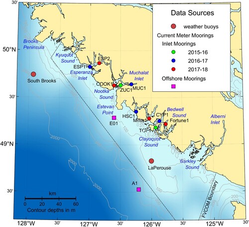
Except in the vicinity of Brooks Peninsula, the bathymetry off western Vancouver Island is characterized by an extensive shelf, steep slope, and broad continental rise (Fig. 1). The shelf has numerous shallow banks separated by a series of deeper basins and/or canyons and, as delineated by the 200-m depth contour, a maximum width of approximately 65 km westward of Juan de Fuca Strait, which narrows northward to about 5 km off Brooks Peninsula. The coastline is also highly convoluted with numerous sounds (Barkley, Clayoquot, Nootka, Kyuquot) and deep inlets (Alberni, Muchalat) penetrating over 50 km into the interior of the island.

Flows off western Vancouver Island primarily consist of tidal currents, wind-generated currents, the buoyancy-driven Vancouver Island Coastal Current (VICC), and a seasonal shelf break current. Freeland et al. (1984), Thomson (1981), and Thomson et al. (1989) have described the origins and nature of the latter two currents. The tides have been extensively measured and their general characteristics have been discussed in Crawford and Thomson (1984), Flather (1988), FT1997 and CMF2000. Virtually continuous current metre deployments have been maintained off Barkley Canyon, Estevan Point and Brooks Peninsula since the early 1980s (R.E. Thomson, personal communication), while other current observations have been taken as part of projects such as the Coastal Current Experiment (Hickey et al., 1991; Thomson et al., 1989) and the La Pérouse Project (Ware & Thomson, 1993).

To evaluate currents simulated by this numerical circulation model, ten acoustic Doppler current profiler (ADCP) moorings were deployed, each for approximately one year between July 2015 to July 2018 (locations are shown in Fig. 1). As mentioned above, two semi-permanent ADCPs collected data on the continental shelf or slope during this time. Although A1 is just outside the domain of the circulation model, both it and E01 off Estevan Point will be used to evaluate the accuracy of this model and the larger domain model that provided boundary forcing.

Finally, model simulations were restricted to the period of 1 March to 31 July 2016. This time period covers the migration of juvenile wild salmon from natal streams seaward past farms that may be infected with sea-lice (Elmoslemany et al., 2015) and extends just past the recovery of the first set of ADCPs in mid-July 2016. It also includes the winter to summer transition in (i) downwelling favourable to upwelling favourable winds along the continental shelf, (ii) heavy rainfall to drought dominated river discharges, and (iii) predominantly seaward outflow winds to predominantly daily sea breezes in many inlets. Moreover, although the presence of the “warm blob” in the Northeast Pacific (Bond et al., 2015; Jackson et al., 2018) meant that 2016 can not be considered typical from a physical oceanographic perspective, output from this simulation does allow a partial assessment of seasonal variations in the wind- and buoyancy-driven currents.

The manuscript is organized as follows. Section 2 briefly describes the circulation model along with the atmospheric, river discharge, and open boundary data that are used to initialize and force it. Section 3 provides an extensive evaluation of the model sea surface heights (SSHs) and currents against available observations. Section 4 discusses sources of inaccuracy, along with changes that should reduce them, while Section 5 presents a brief summary and progress toward the long-term goals of the study. Two appendices respectively provide more detail on freshwater forcing for the model and an evaluation of its temperature and salinity.

2 Model development

The circulation model used in this study is the Finite Volume Community Ocean Model (FVCOM) developed by Chen et al. (2003, 2006a, 2006b, 2011). FVCOM solves the 3D hydrodynamic equations for velocity and surface elevation and 3D transport/diffusion equations for salinity and temperature in the presence of turbulent mixing. It also employs a variable resolution triangular grid in the horizontal direction to provide more flexibility than a regular rectangular grid in representing complicated regions such as the coastline and bathymetry off the west coast of Vancouver Island. It can be forced with any combination of tides, wind, river runoff, surface heating, and open ocean inflows and though they are not used here, has coupled biogeochemical and sediment transport components. The particular code employed (version 4.1) is more recent than that used in the Broughton Archipelago (Foreman, Czajko, et al., 2009) and Discovery Island (Foreman et al., 2012) simulations. Further details on FVCOM and a more complete list of publications that have used it can be found at http://fvcom.smast.umassd.edu/FVCOM/index.html.

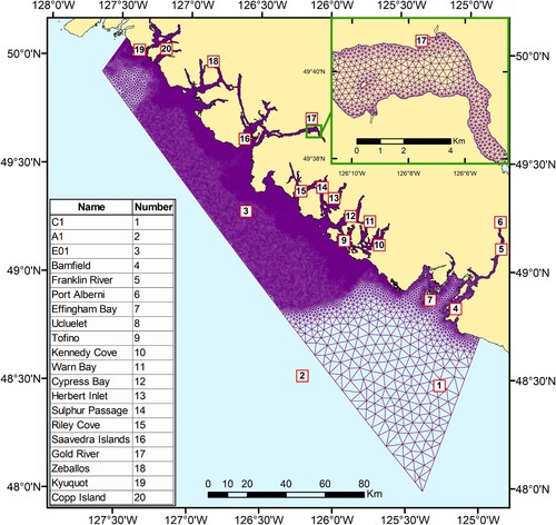
The triangular grid for this FVCOM application has 76,611 nodes, 137,644 elements, and a horizontal grid resolution (smallest element side length) that varies from approximately 60 m in the coastal inlets to 9.2 km at the edge of the continental shelf. It was generated with Matlab© code updating the TriGrid software developed by Henry and Walters (1993). As seen in Fig. 2, there is generally higher resolution in the regions of interest, namely the inlets within, and shelf regions off, Clayoquot Sound, Nootka Sound, and Esperanza Inlet. In the vertical, there are twenty sigma (terrain-following) layers with a hyperbolic tangent distribution that has high resolution at the surface and a maximum inter-layer spacing of approximately 20% of the total depth at the bottom, similar to Foreman et al. (2012). Simulations were also carried out using several hybrid vertical coordinates following the formulation described in Pietrzak et al. (2002). However, in all cases, this sigma-coordinate choice was found to more accurately capture freshwater plumes in the inlets, so only its results will be presented.

Fig. 2 Horizontal grid for the FVCOM simulations and locations of the tide and pressure gauges used to evaluate the model SSHs. The inset shows a grid close-up of eastern Muchalat Inlet near Gold River.

The model bathymetry was generated from Canadian Hydrographic Service (CHS) single-beam acoustic surveys with multi-beam soundings included, where available. Depths (with respect to mean sea level) ranged from drying mudflats in some coastal regions to 200 m on the shelf and as deep as 365 m in portions of Muchalat Inlet. Although shorelines throughout the region are generally steep-sided, there are a few mudflat regions near river mouths, in parts of Clayoquot Sound northeast of Tofino, and on a few beaches (e.g. Long Beach, southeast of Tofino) exposed to the open ocean. At the time the model grid was developed, there was insufficient low-tide topography from Lidar surveys or other sources to assign depths or elevations to these model nodes. However, to provide a preliminary assessment of the role that mudflats play in the local dynamics, simulations were conducted with the wetting-drying capability activated and all mudflat regions assigned a zero depth. Other than in the immediate vicinity of the mudflats, there were only small differences in the tidal harmonics and estuarine flows relative to the simulation when all depths less than 5 m were reset to 5 m so that coastal nodes would never become dry. Moreover, in order to avoid model instabilities and keep the execution time within 160% of that with no wetting-drying, these test runs required both (i) the ratio of internal to external time step be lowered from ten to five (the external time step is 0.15 s), and (ii) the minimum water depth when an element was considered to be dry be increased from the recommended 0.05 m (Chen et al., 2006b) to 0.5 m. Subsequently, results will only be presented for the case with a minimum depth of 5 m. It should be noted that after the zero-depth mudflat tests were conducted, a new source of bathymetry and topography (Davies et al., 2019) became available that should allow for an accurate specification of mudflat wetting-and-drying in the future. This is discussed further in Section 4.

Model bathymetry was smoothed with a volume preserving technique that limits the ratio $\mathrm{\Delta }h/h$ within each triangle, where $\mathrm{\Delta }h$ is the depth range within a cell and $h$ is the average of the depths at the vertices. This smoothing follows Hannah and Wright (1995) and is similar to the criteria recommended by Mellor et al. (1994) and Haney (1991) for reducing “hydrostatic inconsistency” with sigma-coordinate atmospheric and oceanographic models. Although the recommendation for FVCOM models is $\mathrm{\Delta }h/h$ < 0.1 (Chen et al., 2011) when generating a grid with the SMS (Surface Water Model System) grid generation software (http://smsdocs.aquaveo.com/SMS_User_Manual_12.1.pdf), trials similar to those described in Foreman et al. (2012) suggested that $\mathrm{\Delta }h/h$ < 0.5 retained relatively accurate bathymetry and inhibited excessive mixing. That same criterion was used here with the modification that prior to the smoothing and in order to better preserve the generally “U-shaped” cross-inlet depth profiles in narrow steep-sided inlets, such as Muchalat, shoreline depths were reset to the average of those at nodes one element seaward.

The input of freshwater into the model (temperature, salinity, volume discharge) was specified for 29 rivers along the Vancouver Island coast. As daily volume discharges from the hydrometric network maintained by the Water Survey of Canada (https://wateroffice.ec.gc.ca/index_e.html) were available for only six of these rivers, and discharge temperature was only measured by PacFish (http://pacfish.ca/wcviweather/) for a different set of six rivers, approaches had to be developed to estimate values for the others. All discharge salinity was set to zero and the FVCOM parameter “RIVER_TS_SETTING” was set to “calculated”. This means that “the salinity or temperature at discharge nodes is calculated using the mass conservative salinity or temperature equation” (Chen et al., 2006b). Tests with the alternative setting “specified” (wherein the temperature, salinity and discharge are all set by the user, as was done in Foreman et al., [2012]) generally provided poorer agreement with temperature and salinity observations from salmon farms that were closest to river mouths. Further details, including discharge and temperature plots over the period of the model simulation, can be found in Appendix A.

Initial 3D fields of salinity and temperature within the model domain were obtained by spatially interpolating values at 0 : 00 UTC 1 March 2016, from a NEMO (Nucleus for European Modelling of the Ocean; https://www.nemo-ocean.eu) application to the Northeast Pacific Ocean (Lu et al., 2017). This model has 1/36° resolution in longitude and latitude and is presently being run operationally at Environment and Climate Change Canada (ECCC) as part of their western Coastal Ice-Ocean Prediction System (CIOPS-W). As the domain for CIOPS-W includes the FVCOM domain and testing included a hindcast simulation for the period of November 2015 to July 2020, stored values from this test run were used to provide forcing along the FVCOM outer boundary. Specifically, hourly stored CIOPS-W SSHs were interpolated to nodes along the outer boundary and used to provide the elevation forcing. These elevations were referenced to the geoid and included atmospheric pressure. They also included the eight tidal constituents Q1, O1, P1, K1, N2, M2, S2, and K2, their over-tides, and subtidal signals such as the VICC and the Shelf Break Current (Hauke Blanken, personal communication). However, the 2–2.5 km horizontal resolution for CIOPS-W meant that the grid was limited in its representation of the complex coastline, capturing major islands and channels with reasonable accuracy but not all of the smaller inlets. This may have affected its SSH accuracy, not only in inlets and nearshore region, but also along the shelf.

Stored daily 3D CIOPS-W temperature and salinity were also interpolated to these same boundary nodes. However, rather than using them as direct forcing and risking incompatibilities with the SSHs and possible model instabilities, they were weakly imposed through nudging. That is, the boundary FVCOM salinity and temperature were nudged back to the CIOPS-W values with a relaxation time scale of two hours. Eighteen-, three-, and one-hour time scales were also tested, with the latter causing the model to become unstable and the former two not producing as good agreement with the ADCP and Microcat observations at mooring E01. This issue will be discussed further in Section 4 and Appendix B.

Velocity was forced indirectly from the SSH, temperature, and salinity that were specified along the outer boundaries. The FVCOM variable distribution within each triangular grid element has velocity located at the centre while sea surface elevation, temperature, and salinity are at the corners. This means that SSH, T, and S are located on an outer boundary, while velocity can be calculated from the surrounding variables through the momentum equations, albeit with special case approximations for terms like horizontal diffusion whose numerical approximation footprint may extend beyond the model domain. An implicit gravity-wave radiation condition was used for outgoing temperature and salinity signals, while nudging to specified values was used during inflow. A sponge layer with damping that decreases linearly from the boundary to 7.5 km into the model domain was also employed to absorb spurious reflections at the boundary.

FVCOM utilizes the Generalized Ocean Turbulence Model (GOTM; Burchard et al., 1999; Umlauf & Burchard, 2003) and offers several vertical mixing scheme choices. The results displayed herein were obtained with the k-ϵ scheme and a vertical Prandtl number of 1.0 (i.e. the same vertical mixing coefficient is used for viscosity and diffusion). A simulation was also carried out with MY2.5 (Mellor & Yamada, 1982) turbulent mixing to determine the extent to that the mixing parameterization might be influencing vertical profiles in inlets. This issue will be discussed further in the next section. Horizontal diffusion is parameterized with a Smagorinsky (1963) method as described in Chen et al. (2008). Several coefficient values were tested before determining an optimal value of 0.05 m s⁻² in the salinity and temperature transport/diffusion equations and 0.5 m s⁻² for the momentum equations. (In terms of the FVCOM parameters, this means the horizontal Prandtl number was 0.1.) These values provided reasonably smooth velocity fields and minimized the potential contribution of horizontal mixing to vertical mixing in regions with steep bathymetry. Specifically, in FVCOM, horizontal diffusion “occurs only parallel to” the sigma-surface layers and this simplification can lead to overly diffusive model thermoclines and haloclines when those layers have significant slopes (Chen et al., 2006b). This issue will be discussed further in Section 4.

Bottom stress is the product of the bottom velocity, the bottom speed, and a drag coefficient that employs the k-ϵ turbulent mixing scheme and a dynamic dissipation rate equation to calculate the length scale and match a logarithmic bottom layer to the model at a specified height above the bottom. This coefficient was assigned a minimum of 0.0025, consistent with other models (e.g. Foreman et al., 2012). See Chen et al. (2006b) for further details.

The ocean surface was forced with atmospheric pressure, as well as momentum and heat fluxes derived from the 2.5 km, LAMWEST western regional nested model within the High Resolution Deterministic Prediction System (HRDPS) developed and run operationally by Environment and Climate Change Canada (Environment Canada, 2015; https://weather.gc.ca/grib/grib2_HRDPS_HR_e.html). Forty-eight-hour forecasts made four times daily have been archived at the Institute of Ocean Sciences and hourly forcing fields for the duration of the model simulations were constructed by combining six-hour segments between successive predictions and then spatially interpolating them to the FVCOM grid. A comparison of the HRDPS winds with observations at the offshore buoy C46206 is presented in Section 4, along with similar comparisons between model winds and weather observations taken at a salmon farm in 2019. As might be expected, the latter comparison suggests that the atmospheric model’s spatial resolution does not capture topographic impacts on wind speed and direction within the Clayoquot and Nootka Sound inlets and channels, many of whose widths are narrower than 2.5 km. Heat fluxes were computed with standard bulk formulae (Fairall et al., 2003) using air temperature, air pressure, relative humidity, cloud cover, short and long wave radiation from HRDPS, and surface water temperature computed by FVCOM.

3 Model evaluations

The following two sub-sections evaluate model sea surface heights and currents through comparisons with simultaneous and historical observations. Appendix B presents a similar detailed evaluation for model temperature and salinity.

a Sea Surface Heights

1 Tidal

Accuracy of the FVCOM tidal elevations was assessed by comparing constituent amplitudes and phases with their counterparts arising from analyses of tide and pressure gauge observations. Harmonic analyses (Foreman, Cherniawsky, et al., 2009) of stored hourly SSHs over the period of 4 March to 31 July 2016, were used to compute the model amplitudes and phases. The first three days in March were omitted from the analysis to allow for model spin-up and tests were conducted confirming the Foreman and Henry (1989) finding that a 150-day time series is sufficient to adequately separate constituents P1 from K1 and K2 from S2 without inference. The associated observational values were taken from the Canadian Hydrographic Service archives (Anne Ballantyne, personal communication). In this case, only tide or pressure gauges with time series longer than 95 days were chosen, as with suitable inference parameters, this should mean that constituent pairs like K1/P1 and S2/K2 can be adequately separated. Seventeen of the twenty observational time series were from coastal tide gauges while the remaining three were from offshore pressure gauges with the factor 0.9806 used to convert from decibars to metres. All locations are shown in Fig. 2.

Fig. 3 displays model and observed M2 and K1 amplitudes and phases at these twenty sites. The poorest M2 agreement is at Franklin River (#5), Port Alberni (#6), and Gold River (#17), which are near the heads of long deep inlets. In all three cases the model amplitude is too large (by as much as 6%), too late (by up to one hour, approximately 28°), and a similar poor agreement also exists for constituents N2, S2, and K2. This suggests that FVCOM has applied too much damping over the semi-diurnal frequency band. Attempts to improve these inaccuracies by adjusting the minimum bottom friction coefficient, the horizontal viscosity coefficient, and the bathymetric smoothing made little difference, so the source of the problem remains unresolved and will be left for future investigations. However as will be discussed in Section 3.3, the model M2 accuracy at most other sites is comparable to that obtained with previous models in this region. Some of the FVCOM tidal inaccuracy can be attributed to CIOPS-W as SSH forcing along the outer boundary was taken directly from that model. In particular, the first three comparison sites are offshore pressure moorings, which are near the outer boundary and they are seen to have amplitudes that are slightly too small and phases that are too large (late) by approximately 5°. Over all twenty sites, the average amplitude and phase errors for M2 are −0.3 cm and −4.6°, respectively.

Fig. 3 Comparison of M2 (a) and K1 (b) amplitudes (cm) and phase lags (degrees, UTC) at the twenty comparison sites shown in Fig. 2.

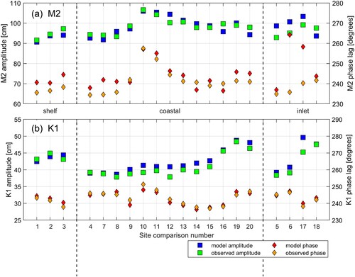
In terms of constituent K1 (Fig. 3a), the model amplitudes and phases are in good agreement with observations at most coastal and inlet sites. In particular, the considerably better agreement than for M2 at site #s 5, 6, and 17 suggests that the FVCOM over-damping in Alberni and Muchalat Inlets is frequency dependent. As with M2, there is a suggestion of a slight bias in the CIOPS-W K1 harmonics at the first three sites. Over all twenty sites, the average amplitude and phase errors for K1 are −1.1 cm and 0.1°, respectively. With regard to site 17 (Gold River) it should be noted that Muchalat Inlet has a regular summer sea breeze and associated SSH response that is aliased with the diurnal tides. No attempt was made to separate these two signals; however, a comparison of HRDPS 2.5 km winds with observations taken in 2019 near the ADCP mooring MUC1 (Fig. 1) showed the former to underestimate the latter by an approximate factor of two. It is reasonable to expect a similar inaccuracy in 2016 causing our simulation to underestimate the associated SSH signal. Further analysis would be required to determine if the timing of the SSH component of the daily sea breeze reduces the K1 amplitude, as indicated in Fig. 3a. Nevertheless, this aliasing likely accounts for at least some of the K1 amplitude difference seen at site 17. Further implications of this sea breeze are discussed in Section 5.

2 Sub-tidal

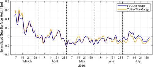
Though tides typically account for over 95% of SSH variance within the model domain, it is important to also assess non-tidal variability as it arises primarily from wind and buoyancy effects. Fig. 4 compares low-pass moving-average filtered (Godin, 1972) SSHs measured at the Tofino tide gauge (site 9 in Fig. 2) with model values over the period of 4 March to 31 July 2016. (Emery and Thomson (2014) showed this filter to have a cut-off period of 66.5 h.) Neither time series was corrected for the inverse barometer effect as atmospheric pressure was included directly in the FVCOM model forcing. A correlation (R) of 0.96 between the two time series indicates overall excellent agreement. Similar correlations (not shown) using bottom pressures recorded by Microcat conductivity-temperature-depth (CTD) instruments at the E01 and ZUC1 ADCP mooring locations (until they stopped on 11 July 2016) were 0.88 and 0.85, respectively, reflecting very good agreement. However, a similar calculation between bottom pressures at the A1 mooring, which is outside the model domain (Fig. 1), and SSHs from the nearest node on the model boundary produced a correlation of only 0.20. Further investigation revealed this discrepancy is not due to the model but rather differences in on-shelf and off-shelf dynamics. Overlaying plots (not shown) of low-pass filtered pressure deviations (from average) for E01 and A1 for the period of 5 August 2015 to 10 July 2016 showed the former to have a seasonal jump of approximately 0.35 decibars during the downwelling season (in this case, 1 December to 25 March) that was essentially nonexistent in the latter. This is consistent with the jump in average winter-summer SSH difference along ground track 86 of the TOPEX-Poseidon-Jason satellite altimeter (Fig. 4 in Foreman, Crawford, et al., 2008) that crosses the continental shelf just south of our model domain. The implication is that SSH (and bottom pressure) along the shelf exhibit(s) a marked seasonal difference due the transitions between downwelling and upwelling winds that is not found off the shelf. As our model domain lies completely on the shelf (Fig. 1), it is, therefore, not surprising that pressure time series along its western boundary have different patterns from, and a low correlation with, those at mooring A1.

Fig. 4 Hourly, low-pass filtered, observed and model SSHs at Tofino for 4 March to 31 July 2016. Both time series have been normalized so their respective means are zero.

b Current Evaluations

Model current accuracy was assessed through comparisons with observations from ten of the ADCP deployments shown in Fig. 1. As moorings E01, TOF1, and ZUC1 were in the water during most of the March-July 2016 simulation time period, model versus observed comparisons can be made with both the tidal and sub-tidal components of their flows. However, as ESP1, CYP1, and MUC1 were in the water in March-July 2017 while Millar1, Fortune1, COOK1, and ESP2 were measuring in March-July 2018, only the tidal components of their flows will be compared with those from the 2016 model simulation, with the underlying assumption that the tides should exhibit a high degree of seasonal and interannual consistency. E01 was redeployed for both these later time periods and as its March-July sub-tidal flows exhibited considerable inter-annual variability, the 2016 model sub-tidal flows at ESP1, CYP1, MUC1, Millar1, Fortune1, COOK1, and ESP2 were not compared with those observed. Unfortunately, mooring HSC1 (Fig. 1) which was deployed at the same time as ESP1, CYP1, and MUC1 failed in December 2016 so it had no March-July 2017 measurements for a model comparison.

1 Tidal current comparisons

Fig. 5 compares observed and model (at the nearest grid element) M2 and K1 major semi-axes at moorings E01, TOF1, and ZUC1. In all cases, harmonic tidal analyses of hourly data from 4 March to 11 July 2016, were used to compute the ellipse parameters for each constituent. Instances where the model values do not extend as deep as the actual depth are due to depth smoothing and the fact that FVCOM velocities are halfway down each layer, rather than at the bottom. Model values extend to the surface layer while the associated observed speeds are omitted due to signal contamination in the near-surface bins. ADCP bin depths were 4 m for E01, 1.5 m for TOF1, 2 m for the top mooring at ZUC1 and 8 m for the bottom.

Fig. 5 Observed and model M2 and K1 major semi-axes versus depth at (a) E01, (b) TOF1, and (c) ZUC1 as determined by harmonic analysis of hourly values over 4 March to 11 July 2016. Note scale changes.

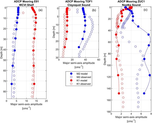
The most notable feature of the major semi-axis values at mooring E01 is that K1 is larger than M2 (Fig. 5a). This is due to the diurnal shelf waves that are generated near the entrance to Juan de Fuca Strait and propagate to the northwest beyond Brooks Peninsula (CMF2000). These waves have been studied extensively (e.g. Crawford & Thomson, 1984) and except at 5 m depth where observed values may still contain some near-surface contamination, the model captured both the magnitudes and relatively constant speeds over the entire water column with reasonable accuracy. The M2 comparison is not as good but still quite similar to the observations (with model values being slightly larger than their observed counterparts at mid-depth and smaller below). Further discussion of the shelf wave accuracy in this model can be found in Section 3.3.

Interpolating the FVCOM layer values to the observed bin depths and ignoring the top bin (4.95 m) where the observations are suspect, allowed a quantitative comparison of the observed and modelled values shown in Fig. 5a. The M2 FVCOM major semi-axes were found to be too large, by up to 32%, in the upper half of the water column and too small, by up to 34%, in the lower half. The model and observed averages over the water column below 4.95 m only differed by 0.6%. This suggests that although the E01 observations are essentially barotropic, the model has also included a baroclinic component with mode 1 variability. The K1 agreement is much better. Except at three bin depths around 50 m where they are slightly smaller, the model values are consistently larger with the largest difference being 10% at 8.95 m. Again, both profiles are seen to be essentially barotropic with the water column averages differing by only 3.9%.

A similar comparison at TOF1 (Fig. 5b) shows that M2 is the dominant constituent. While the M2 model speeds are too small by up to 20% over most of the water column (observed values for the top two bins may be contaminated), their K1 counterparts are too large by approximately the same percentage. Interpolating the M2 FVCOM layer values to ADCP bin depths in the range of 3.89 m to 23.89 m and comparing observed and model values (as was done at E01) reveals that except for the value at 3.89 m, the model M2 major semi-axes are 16% to 23% too small. However, the model has captured the shape of the observed profile with both having maximum speeds at around 10 m depth. This is not the case for K1 where the model values are consistently too large, with the discrepancy decreasing monotonically from 50% at 5.39 m to 16% at 23.39 m.

Tidal speeds at the ZUC1 mooring (Fig. 5c) are seen to be considerably smaller than those at TOF1. The ADCP profiles combine data from two instruments: the deeper one sampling at 150 kHz providing data in 8 m bins from 172 to 34 m depth, and the shallower one sampling at 300 kHz providing data in 2 m bins from 34 to 2 m depth. The M2 model major semi-axes are seen to be too large over most of the water column and have a depth profile that is quite different than that observed. Specifically, the model speed maximum at about 45 m is too shallow relative to the observed at approximately 85 m. Although plots comparing model and observed M2 ellipse angle of inclination show agreement to within 10° and relatively constant values that align with the channel direction, a plot of ellipse phase lag shows values that are too small (early) by approximately 40° over the top 30 m of the water column and too large (late) by between 25° and 50° below 60 m depth. These speed and phase inaccuracies suggest the model has not captured the mode 1 component of the M2 baroclinic tides correctly; a result that might be expected given that (as will be seen in Section 3.2.2) the model low-pass filtered flows (Fig. 9b), and model salinity and temperature at 184 and 40 m (Fig. B7), are also inaccurate.

As the associated K1 major semi-axes are relatively small, the discrepancy between model and observed values in Fig. 5c also seems small. However, when viewed as percentage discrepancies, they are as poor as those for M2. Between 5.77 and 80 m, the model speeds are too large by as much as 75%, while below that depth they are too small by as much as 38%. As for M2, it is likely that this poor model accuracy is related to the poor representation of the estuarine (and perhaps wind-driven) flows. Further work is needed to improve both the estuarine and semi-diurnal tidal flows in this region, which will likely require a combination of grid refinements, modifications to the bathymetry, further investigation of mixing parameterizations, and changes to the prescription of river discharges. See Section 4 for further discussion on this issue.

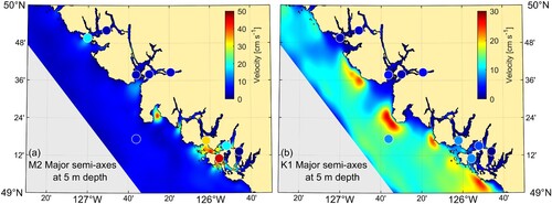
In Fig. 6, the spatial distribution of modelled M2 and K1 major semi-axes at 5 m depth are compared with analogous values from the ADCP moorings at the bin closest to 5 m. Values for the E01, TOF1, and ZUC1 moorings were computed via harmonic analyses (Foreman, Cherniawsky, et al., 2009) over the simulation time period, namely 4 March to 11 July 2016, while those for the other moorings were for different years but covered the same time period. Although perfect seasonal stationarity in the tidal currents is unlikely, we are assuming the year-to-year changes will be small. While the M2 speeds are relatively small along the shelf, they increase substantially in the generally shallow entrances to the Clayoquot Sound inlets, and to a lesser degree in the deeper entrances to Nootka and Esperanza Sounds. Agreement between the model and observed values is seen to be reasonable, at least at 5 m depth, given the high spatial variations shown in the model results. The previously studied (Flather, 1988; FT1997) trough/peak wavelength pattern of diurnal shelf waves has been captured by the model and is seen to extend into the inlets. The next section discusses K1 shelf wave accuracy further.

Fig. 6 Model M2 (a) and K1 (b) major semi-axes (cm s⁻¹) at 5 m depth with comparable values from ADCP time series at the bin closest to 5 m, super-imposed as coloured dots. (See Fig. 1 for precise ADCP locations.)

Table 1 displays M2 and K1 model and observed semi-major axis values at these same ten moorings and at bin depths, or FVCOM layer depths, closest to 5 m. Those for the model time series were obtained from harmonic analyses for the period of 4 March to 11 July 2016. Agreement is seen to vary between good for some sites and constituents (e.g. M2 at E01), to poor at others (e.g. K1 at Fortune1). In some instances, the discrepancy may be explained by near surface bin contamination (e.g. K1 at E01, as suggested by Fig. 5a) or model values that have been compromised by nearby coastline or depth approximations and/or depth smoothing. In other cases, like Fortune1, agreement is better at 12 m depth and below where near-surface aliasing from features like a daily sea breeze have contaminated the observed and model tidal analyses to different extents because the HRDPS forcing does not represent these winds well. This issue is discussed further in Sections 4 and 5. In general, the accuracy of tidal ellipse parameters like major semi-axis is seldom as good as amplitude and phase for tidal elevation (e.g. FT1997). In that regard, the agreement or lack thereof with this model is typical.

Table 1. M2 and K1 major semi-axes (cm s⁻¹) at the ADCP moorings displayed in Fig. 1 and at the bin depths, or FVCOM layer depths, closest to 5 m.

Site	M2 obs	M2 mod	K1 obs	K1 mod	obs year	obs depth (m)	mod depth (m)	depth dif (m)
E01	6.23	5.83	8.36	14.20	2016	4.95	4.50	0.45
TOF1	46.37	38.83	8.31	12.49	2016	5.39	5.31	0.08
ZUC1	3.92	3.69	2.09	2.40	2016	5.77	4.86	0.91
COOK1	3.64	4.84	4.44	2.42	2018	4.81	4.78	0.03
CYP1	18.78	22.17	6.20	7.69	2017	5.80	5.80	0.00
ESP1	18.10	10.84	2.00	0.83	2017	5.80	5.00	0.80
ESP2	2.83	5.24	2.34	2.26	2018	4.78	4.11	0.67
Fortune1	5.53	11.67	6.76	1.36	2018	5.99	5.42	0.57
Millar1	33.33	40.82	8.41	12.02	2018	5.05	5.32	−0.27
MUC1	4.20	5.34	3.40	0.98	2017	5.21	4.13	1.08

2 Sub-tidal current comparisons

Directional histograms (not shown) were computed for the March through July currents observed at all bins of each of the ten moorings and showed dominant flow directions that, in general, were strongly aligned with along-channel or along-shelf bathymetric directions. Fig. 7 shows the 4 March to 11 July 2016, along-shelf current profiles for the E01 mooring after the same low-pass moving-average filter applied to the SSHs was also used to remove tidal currents. Comparable profiles from both the FVCOM and CIOPS-W (data courtesy of Hauke Blanken) models have also been included to assess model differences. Note that the CIOPS-W and FVCOM values rise to within 0.5 and 0.01 m of the surface respectively, while the ADCP velocities were cut-off at 8.95 m as velocities from bins above that depth were deemed unreliable.

Fig. 7 Along-shelf, low-pass filtered velocity profiles (m s⁻¹) at the E01 mooring for 1 March to 11 July 2016: (a) observed with bottom mounted ADCP, (b) simulated with CIOPS-W model, (c) simulated with FVCOM model. Positive (red) velocities are directed toward 147°counter-clockwise from east and are typically associated with downwelling conditions. Negative (blue) velocities, directed toward 33° clockwise from east, are similarly associated with upwelling conditions. Grey regions denote unreliable observations.

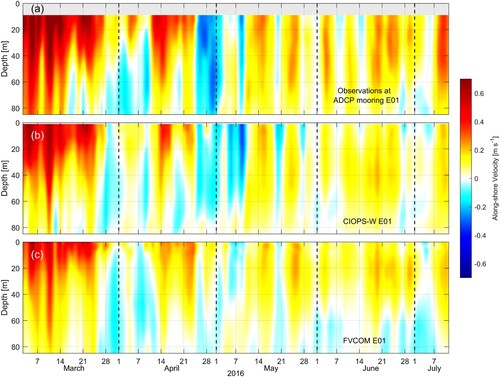
Except during periods of strong upwelling winds (e.g. late April), the E01 low-pass filtered currents were generally northwestward with some speeds exceeding 0.6 m s⁻¹. As this mooring lies within the VICC (Thomson et al., 1989), the low-pass filtered currents are primarily driven by winds, surface estuarine outflows from Juan de Fuca Strait, and freshwater discharges from the coastal inlets. These currents are much larger in the winter and early spring when the winds are generally stronger and blowing in the same direction as the VICC, and typically persist in summer, albeit weaker when upwelling-favourable winds oppose the VICC northwestward flow. However, reversals can occur over portions of, or the entire, water column. Note the reversal in late April 2016, which roughly corresponded with the spring transition from generally downwelling-favorable to generally upwelling-favorable winds, and another around 10 May, which coincided with the strongest upwelling HRDPS winds at offshore weather buoy C46206. (See Fig. 11 and associated text in Section 4 for further discussion.)

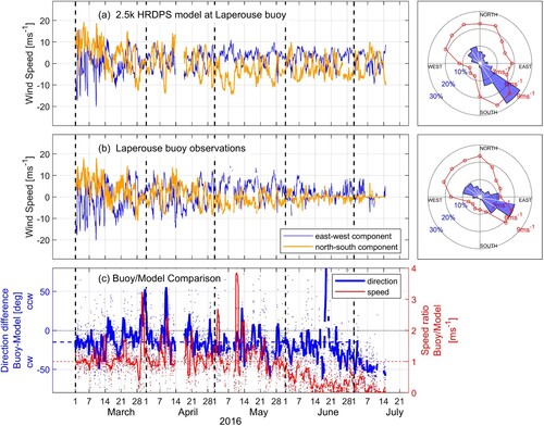
Fig. 11 East-west and north-south components of the wind (m s⁻¹) (left column) and wind roses (right column) at the La Perouse buoy (C46206 in Fig. 1) for the period of 1 March to 15 July 2016. Row (a) shows the east-west and north-south components from the HRDPS model and the associated wind rose, while row (b) is similar but for the observations. Row (c) displays differences in direction and speed ratios. Dots are hourly values while lines are twelve hour running means. Wind rose directions denote to where the wind is blowing while the polygons denote the average speed in each direction.

While both models underestimate the strength and depth of the northwestward flows in the first three weeks of March and in mid-April (Fig. 7), the observed sub-tidal variability has been captured. Both CIOPS-W and FVCOM also underestimate the strong upwelling at the end of April yet CIOPS-W over-estimates the subsequent shorter upwelling period around 10 May, while FVCOM underestimates it. Specifically, CIOPS-W shows a longer period of upwelling starting earlier, and overall larger velocities that do not extend as far down the water column, while FVCOM better captures the upwelling duration but not the depth of the southeastward currents. And although the magnitudes and water column extent of the generally northwestward flows observed from mid-May to mid-July are underestimated by CIOPS-W, the timing of their variability was replicated with reasonable accuracy. The comparable FVCOM currents are seen to be in slightly better agreement with the observations but have short episodes of southeastward flow over the entire water column that were not present in the ADCP values. As both CIOPS-W and FVCOM have the same HRDPS atmospheric forcing, different results from these two models must arise from a combination of grid resolution, freshwater discharge, and forcing along the outer boundary of FVCOM. Also, CIOPS-W includes one river discharge into each of the Barkley Sound, Clayoquot Sound, Nootka Inlet, and Kyuquot Sound regions (Li Zhai, personal communication) and the flows are climatological averages. Given that FVCOM takes SSHs along its outer boundary from CIOPS-W, the respective, mainly barotropic, flows should be very similar. However, the baroclinic flows could differ as FVCOM only nudges back to daily CIOPS-W temperature and salinity values along its outer boundary. As will be discussed later in Section 4, the nudging may not be sufficiently strong, i.e. the e-folding time scale may need to be smaller.

It is important to point out that local winds are not the only forcing mechanism driving the along shore flow. The Vancouver Island Coastal Current and remote winds can also play important roles. Engida et al. (2016) showed that the 35 m currents at mooring A1 were most highly correlated with time-shifted winds along the Washington and Oregon coasts, rather than local winds. This means that it is important for CIOPS-W, and/or the parent model that provides boundary forcing to CIOPS-W, to accurately represent both the VICC and currents generated by these remote winds in the vicinity of the southern boundary of the FVCOM domain.

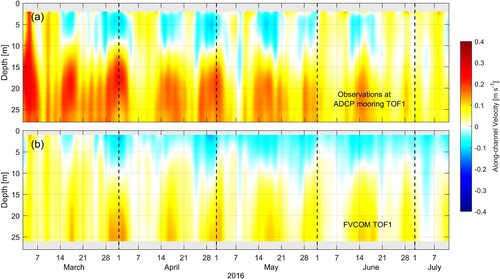
Similar comparisons between the ADCP observations and FVCOM model currents are shown in Fig. 8 for the TOF1 mooring. (The CIOPS-W profile has not been included as that grid does not adequately capture the inlet where TOF1 is located.) In order to extend the observations closer to the surface and overcome data gaps in the near surface bins, the data were interpolated to 2 m depth. Although both plots reveal what is generally a two-layer estuarine flow with a notable fortnightly modulation, the model bottom flows are seen to be too weak. This suggests insufficient input from the shelf region which in turn may be related to a too-weak VICC and insufficient temperature-salinity nudging along the southern boundary.

Fig. 8 Along-channel, low-pass filtered velocity profiles (m s⁻¹) at the TOF1 mooring: (a) observed with bottom mounted ADCP, (b) simulated with FVCOM model. Positive velocities are directed toward 57° counter-clockwise from east. Grey regions denotes unreliable observations or missing values due to bathymetric smoothing.

Although tidal spectra on the continental shelf generally show that diurnal are typically larger than semi-diurnal currents (Crawford & Thomson, 1984; Foreman & Thomson, 1997; CMF2000), the semi-diurnals are considerably larger within Clayoquot Sound. Spatial variations and specific tidal currents magnitudes were discussed previously, but at TOF1 the relatively large semi-diurnals produce interesting results in the low-pass filtered currents seen in Fig. 8. Specifically, while significant variations in low-pass filtered currents are usually due to a combination of winds and local freshwater discharge events, a visual comparison with simultaneous nearby wind and freshwater discharge time series (not shown) reveals little correlation. Rather, fortnightly variations in both the upper and lower layer flows align with the spring-neap tidal cycle at the Tofino tide gauge (e.g. neap tides around 17 and 31 March and 16 and 30 April). This suggests that smaller tidal mixing during neap tides allows pulses of fresher near-surface water from the numerous rivers discharging into the Clayoquot inlets to move seaward, while stronger mixing during spring tides greatly reduces that buoyancy flow. Salinity and temperature measured by the near-bottom Microcat at TOF1 (Appendix B) reveal that during neap tides, the water is cooler and more saline, consistent with stronger bottom flows entering from the shelf to balance the stronger near-surface outflows. Griffin and LeBlond (1990), Hickey et al. (1991), and Soontiens and Allen (2017) describes a similar phenomenon from the surface perspective, namely fresher water pulses escaping from the Strait of Georgia and moving seaward into the Strait of Juan de Fuca during neap periods.

As mentioned earlier, two upward looking ADCPs were deployed at the ZUC1 mooring. As in Fig. 5(c) and 9(a) displays observations from the bottom instrument over the depth range of 34 m to the bottom and from the top instrument from 34 m to 2 m below the average surface. Near-surface, along-channel, low-pass filtered flows are seen to frequently reverse between the up- and down-channel directions. As the tides are much weaker here, these flows are primarily driven by a combination of winds, both off the coast and locally in the inlets, and to a lesser extent, freshwater discharges further upstream in the inlets. For example, the Gold River discharge peak on 7 April (Fig. A2) has likely contributed to the larger down-channel (negative) 0–15 m event that is seen in the ZUC1 low-pass filtered flows on 10 April. Note there are many relatively strong near-surface outflows at other times that do not correlate with the Gold River discharges. There is also some correlation between stronger upwelling winds measured at the offshore buoys and seaward flow at ZUC1 (not shown). Such winds produce an elevation set-down along the coast, a larger difference in dynamic height between up-inlet and coastal values, and thus larger compensating seaward flows. The time series of low-pass filtered elevations from the Tofino tide gauge (Fig. 4) has relatively high variability with minima generally corresponding to stronger upwelling-favourable winds (e.g. 10 May) and maxima corresponding to either stronger downwelling-favorable or onshore (positive cross-shore) winds. Specifically, Fig. 11 in Section 4 shows the east-west and north-south components of the winds at offshore buoy C46206. Strong upwelling winds are seen in the HRDPS time series on 30 April and from approximately 6 May to 10 May while strong downwelling winds are seen on 6 March and 8 March.

Fig. 9 Along-channel, low-pass filtered velocity profiles (m s⁻¹) at the ZUC1 mooring: (a) observed with bottom mounted ADCP, (b) simulated with FVCOM model. Positive velocities (red) are directed up-inlet toward 71° counter-clockwise from east. Grey regions denote unreliable observations or missing values due to bathymetric smoothing.

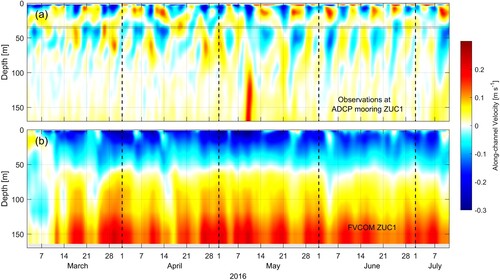
It takes approximately fifteen days before the model velocity profiles at TOF1 and ZUC1 show some similarities with the observations. This is due to inaccuracies in the initial temperature and salinity fields (recall the CIOPS-W limited resolution in the coastal inlets) and the time required for the forcing fields (atmospheric, tidal, freshwater discharge) to overcome them. However, as seen in Fig. 9(b), even after this time period the model flows at ZUC1 display limited agreement with the observations. While the model profile shows some up-inlet near-surface events, they are fewer than what were observed. Rather there is relatively consistent seaward flow over the top 50 m as opposed to the frequently reversing two-layers over the top 60 m. Furthermore, whereas the observations show relatively weak currents below 100 m (apart from the 10 May event to be discussed shortly), the model has much stronger up-inlet flow at depth in order to compensate for the larger near surface outflows. Although a reasonable explanation for the too-strong surface flows would be too much freshwater discharge further up Nootka Sound and in Muchalat Inlet, subsequent evaluations of model and observed near surface salinity (Appendix B) indicate that in fact, the model overestimates near surface salinity in this region. Further discussion follows in Section 4.

Fig. 9a shows that there can be as many as four layers flowing in different directions from those above or below. The dynamics behind the multi-layer flows under those at the surface are complex and may be similar to those observed in Douglas Channel (Wan et al., 2017). The large up-inlet spike in the bottom currents on 9–10 May is, in all likelihood, a density intrusion that arose after several days of upwelling winds and in particular, the strongest winds and lowest SSH at Tofino (Fig. 4) on 30 April and a rapid rise in SSH on 10 May. The associated Microcat temperature time series at 185 m (Appendix B) reveals a simultaneous sharp change to cooler temperature, not only at this time but also in early July when there is another, albeit weaker, increase in up-channel flows below 100 m depth (bottom right corner of Fig. 9a). Fig. 9b shows that although the model does have strong bottom and surface currents during this same period, it also has similar strong currents at many other times. As such, it is unlikely the intrusion dynamics were captured correctly. This is discussed further in Appendix B.

c Accuracy Comparison with Previous Models

Most previous regional models that included the west coast of Vancouver Island were either barotropic (e.g. Flather, 1988; Foreman et al., 2004), steady-state baroclinic wherein the three-dimensional density field was prescribed but remained constant in time (e.g. FT1997), or baroclinic but with too coarse a horizontal grid to resolve the inlets (e.g. CMF2000; Masson & Fine, 2012). Those resolving the inlets employed unstructured triangle grids similar to here but because they were either barotropic or their density was not fully prognostic, they avoided the possibility of baroclinic instabilities (Haney, 1991) and, therefore, the need for bathymetric smoothing. This meant that their tidal height amplitudes and phases were generally more accurate. On the other hand, some of the inaccuracies seen in Fig. 3 can be attributed to bathymetric smoothing. For example, the M2 phase inaccuracy is seen to grow appreciably between Franklin River and Port Alberni (sites 5 and 6) in upper Alberni Inlet where depth smoothing has reduced the average depth from 55 m to 35 m. According to the analytic solutions given by Lynch and Gray (1978), this depth change translates to an additional phase lag of 8°. Although this is much less than the 27° discrepancy calculated by our model, Lynch and Gray (1978) had linear bottom friction as their only dissipation mechanism, whereas this FVCOM application had not only quadratic bottom friction, but also both horizontal and vertical viscosity. The point is that the time-evolving temperature and salinity fields, when combined with terrain-following vertical coordinates and steep bathymetry, necessitate smoothing or other bathymetric adjustments to maintain stability and those can affect the accuracy of dynamics like tidal heights.

FT1997 evaluated the accuracy of their tidal heights using the metric D, the distance between the observed and modelled complex amplitudes Ae^(−ig), where A is the amplitude and g is the phase lag. Although their model domain extended beyond the one here (Fig. 2), the average Ds for M2 and K1 over all forty-three sites used their evaluation were 3.1 and 1.7 cm, respectively. These values are less than the 5.8 and 2.7 cm values for the fully-baroclinic FVCOM application to the Broughton Archipelago (Foreman, Czajko, et al., 2009) and the 3.8 and 3.5 cm values for the fully-baroclinic FVCOM application to the Discovery Islands (Foreman et al., 2012). M2 average D values for the twenty sites in this application are considerably larger at 9.9 cm. But if the Port Alberni and Gold River sites are omitted, the average drops to 6.5 cm, comparable to that for the Broughton Archipelago application, which like this application also has deep fjords and a complicated coastline. However, the average D over all twenty sites for K1 is 1.7 cm, the same as that calculated for FT1997 and less than that for both the Broughton and Discovery models. So relative to previous models in the Vancouver Island region, the K1 tidal height accuracy is as good or better, while the M2 accuracy is somewhat worse. Further discussion on the accuracies in these models is given in Section 4.

With regard to tidal current accuracy, previous models for this region either did not resolve the inlets or did so with limited resolution. Therefore, accuracy evaluations using inlet observations from locations such as those shown in Fig. 2 (except E01) would not be fair. However, it is fair to compare with observations on the shelf, and in particular to evaluate how well this model captured the K1 continental shelf wave that has been the focus of previous of modelling and observational studies (Crawford & Thomson, 1984; Flather, 1988; CMF2000). These studies established that the diurnal shelf waves are generated at the entrance of Juan de Fuca Strait, which is just beyond the southern boundary of our model. This means that their accuracy in the FVCOM model is a function of how well (i) CIOPS-W captured the wave generation near the strait entrance, (ii) the shelf wave signal was transmitted through the SSH, temperature and salinity forcing along the southern, and to a lesser degree to the western, boundaries of the model, and (iii) their propagation was represented within the model domain.

As the clockwise vector is the dominant rotary component of this wave (Crawford & Thomson, 1984; Hsieh, 1982), we followed the example of FT1997 and CMF2000 and calculated the co-amplitudes and co-phases of that component at 30 m, the depth at which many of the historical observations were taken. This means that the FVCOM results (not shown) can be compared to the model and observed values shown in Fig. 5 of FT1997 and Fig. 9 in CMF2000. Note that the FT1997 model was barotropic while CMF2000 conducted both barotropic and baroclinc simulations in order to demonstrate that the inclusion of stratification improved the K1 alongshore phase propagation of both rotary components. Specifically, CMF2000 found that with homogeneous density, shelf waves propagated relatively slowly and were dissipated before reaching Brooks Peninsula; whereas, with a typical summer stratification the waves propagated beyond Brooks Peninsula and were in better agreement with observations.

The first feature to check with our FVCOM simulation is accuracy near the southern boundary. In that respect, all FVCOM values lay within the range of those observed at the seven sites displayed in Fig. 5 of FT1997, namely co-phases are between 169° and 204° and co-amplitudes are between 7 and 11 cm s⁻¹. Although CMT2000 only displayed one set of observations in that region, they were also within those ranges. We, therefore, conclude that both CMF2000 models and FVCOM have accurately captured the K1 shelf wave just downstream of their generation. Further along the shelf, all models produced peak clockwise current speeds of 15–18 cm s⁻¹ mid-shelf south of Tofino with the CMT2000 barotropic speeds being larger than the baroclinic. Finally, the CMF2000 along-shelf plots of the clockwise co-amplitudes and co-phases for both homogeneous and typical summer density (their Fig. 9) are comparable to Fig. 5 in FT1997 and to analogous versions produced (but not shown) for this model. The fact that our FVCOM simulation spans March to July and our domain does not extend to the northern end of Vancouver Island, introduces caveats on a direct comparison of results. That said, our 360°-to-0° co-phase transition occurs between Esperanza Inlet and Kyuquot Sound (see Fig. 1), in approximate agreement with the CMF2000 stratified result, and in contrast to their homogeneous density case that has the same transition further south between Estevan Point and Nootka Sound and to the barotropic FT1997 result that has the transition just north of Nootka Sound. Unfortunately, there are no observations between Estevan Point and Brooks Peninsula so we cannot quantify accuracy of the FVCOM shelf wave in that region. However, the fact that its co-phases are close to those for the baroclinic CMF2000 case, and those results were accurate further downstream at Brooks Peninsula, indicates the FVCOM application has accurately captured K1 shelf wave propagation over the extent of its model domain.

4 Analysis of model inaccuracies

In this section, we summarize major sources of inaccuracy in the foregoing simulation and describe measures that could be adopted to reduce them.

a Steep Bathymetry in Narrow Inlets

Although the channels where moorings TOF1 and ZUC1 were located have a similar width, the latter is much deeper, has much weaker tidal currents (Fig. 9) and different mixing dynamics. It is well known (e.g. Haney, 1991) that terrain-following coordinates combined with steep bathymetry not only cause over-mixing, but can also, in extreme cases, lead to model instabilities. This is certainly an issue with this model domain where for example, Muchalat Inlet attains depths greater than 300 m and is only between 1 and 2.5 km wide. While we have attempted to alleviate this problem by smoothing our bathymetry and resetting some shoreline depths to the average of those at nodes one element seaward, in all likelihood there is still over-mixing in many inlets. In particular, reducing the Δh/h threshold from 0.5 to 0.3 or lower would induce more smoothing near the coast, deepening the coastal depths and reducing the maximum depths in the middle of the inlet. As described in Section 3.3 for upper Alberni Inlet, this would change the hydrodynamics and accuracy of features like the barotropic tide. Recent work in Bute Inlet (on the mainland BC coast in the Discovery Islands region) has demonstrated that this mixing can be reduced by diminishing or removing the steepness of the bathymetry across-inlet, such that it mostly varies along the thalweg while remaining relatively flat along the cross-sections (Bianucci et al., in preparation). This approach, which maintains acceptable Δh/h values, while eliminating the need for smoothing, reduces the large depth gradients that previously existed near inlet coastlines and has been designed to preserve cross-sectional areas so that barotropic dynamics (e.g. tides) are relatively unchanged. Note that special consideration would have to be given to sills and regions near river mouths where for example, a Heaviside specification (an option within FVCOM) of the vertical extent of the river discharge would probably be needed to restrict that discharge to only the upper portion of the water column. Modifications to the coastal inlets in this model domain are planned and those results will be described in a future manuscript.

Note that such bathymetric changes should also reduce inaccuracies arising from a lateral mixing assumption that is made within FVCOM. Specifically, the horizontal diffusion terms are simplified so that this diffusion only occurs parallel to the terrain-following layers (Chen et al., 2006b). This assumption means there will be an additional contribution to the vertical mixing in sloping regions (Chen et al., 2011), which could explain the fact that the model 1 m salinity at sixteen salmon farms within the inlets were, on average, too salty by 2.5 (Appendix B). Specifically, mixing along the shallow layers near the sides of the inlets where the slopes are greatest would certainly make near-surface waters saltier and deeper waters fresher.

b Open Boundary Forcing

The accuracy of the open boundary forcing in this FVCOM application is highly dependent on the accuracy of the CIOPS-W model. Though Fig. 3 suggests a slight bias in the tidal elevations from that model, Fig. B4 indicates that the nudging back to the 3D temperature and salinity from CIOPS-W has performed reasonably well at E01. On the other hand, Fig. 8(b) shows that the model low-pass filtered bottom currents at TOF1 are too weak and this could be due to a combination of CIOPS-W not accurately representing the VICC along the model southern boundary, and the nudging back to those values not being sufficiently strong. More recent hindcasts of CIOPS-W store their temperature and salinity hourly, rather than daily and this should allow smaller time scales for the nudging. This will be explored in future research.

The fact the CIOPS-W SSHs that provided forcing along the outer boundary of the model were only available in hourly increments caused a slight underestimation of the tidal amplitudes. This is because FVCOM performs a linear interpolation between the prescribed SSHs (and indeed all forcing) to obtain values at model time steps and that results in a clipping of the maximum and minimum values. In order to estimate the magnitude of this effect, a time series of hourly SSHs was generated using only the observed M2 and K1 amplitudes and phases for Tofino (site 9 in Fig. 2). This time series was then linearly interpolated to 5-minute sampling and harmonically analysed using the Foreman, Cherniawsky, et al. (2009) software. The resultant M2 and K1 amplitudes were reduced by 2.1% and 0.57% respectively while the phases were unchanged, to the second decimal place. The post-analysis RMS residual error was approximately one percent of the original signal and to the third decimal place, there was no energy leakage to other tidal constituents. Thus, the prescription of hourly (as opposed to more frequent) SSH forcing slightly reduced the FVCOM tidal signal along the outer boundary. But as seen in Fig. 3, those reductions are comparable to, and typically less than, the inaccuracies at many coastal tide gauge locations and would not explain instances where the model amplitudes are larger than those obtained from an analysis of observations. Furthermore, this issue would not explain the fact that the M2 phases at offshore sites 1–3 were too large by approximately 5°.

Certainly, there are inaccuracies in the CIOPS-W tides, and it would not be difficult to both replace them with values from another model and increase their temporal resolution so the previously-described amplitude clipping is reduced. Subtidal energy in the CIOPS-W SSHs could be extracted when the tides were removed and if desired, interpolated to a more frequent sampling before adding back in with the new tides. The subtidal energy has periods longer than diurnal and thus the inaccuracy arising from a linear interpolation of hourly to 5-minute data can be expected to generate errors less than the 0.5% that was estimated for the K1 tide. Candidates to replace the CIOPS-W tides include the regional TPXO9 model for the Gulf of Alaska and Bering Sea (Egbert & Erofeeva, 2002); FES2022, the latest in the French series of high resolution, assimilating global tidal models (Michel Lionel et al., 2023); or one of several larger domain models for the waters around Vancouver Island. A test wherein the M2 and K1 tides in CIOPS-W were replaced with those from the Foreman et al. (2004) model that assimilated tide gauge harmonics from twenty-four tide gauge locations around Vancouver Island produced very little change in model accuracy. Specifically, the average D for the twenty locations displayed in Fig. 3 went from 10.25 cm to 10.05 cm for M2, and from 1.70 cm to 2.05 cm for K1. (As noted previously, the M2 averages are heavily skewed by D values of approximately 30 cm at Port Alberni and 16 cm at Gold River, with the former being larger because Alberni Inlet has a coarser resolution than Muchalat Inlet.)

c Bathymetry

As mentioned in Section 2, new bathymetry and topography (Davies et al., 2019) are now available, which should allow for the accurate specification of mudflat wetting-and-drying. Specifically, five digital elevation models (DEMs) with 20 m horizontal resolution have been created for Canada’s Pacific coastal region using marine depth soundings from Canadian Hydrographic Service, terrestrial elevations from Natural Resources Canada, and a continuous 20 m raster interpolation extending from depths across the intertidal to upland, 5 km from shore. Note that these new data also mean that river channels could be extended upstream to the location of the WSC gauges, thus removing the assumption that WSC discharges do not change from where they are measured to where they reach the coast. Of course, the previously mentioned restrictions on the internal – external time step ratio and the minimum depths at which a cell is deemed to be dry, both of which seem to be needed to overcome large execution times and/or model instabilities, still require further investigation. However, FVCOM has the ability to create sub-domains within a grid where only these restrictions could apply, thereby alleviating the heavy computational costs that would be incurred if they were applied over the entire model domain.

d Vertical Resolution

Another source of inaccuracy can be the choice of vertical layers. The sigma layers employed here were thin near the surface and progressively thicker down the water column in an attempt to better capture the freshwater lens and wind stress transfer that were felt to be important drivers of currents affecting the salmon farms. A potential problem with this distribution is that bottom friction may not be captured accurately, especially in shallow water, and this could affect dynamics like tidal propagation. In order to assess the magnitude of this potential problem, a simulation was conducted with thirty versus twenty vertical layers (albeit using the same formula for their distribution), which reduced the bottom layer thickness by approximately 25%. Comparing the new M2 major semi-axis profile with those shown in Fig. 5(b) for the relatively shallow ADCP mooring site of TOF1, the new model values were seen to be slightly larger (maximum of 40.6 cm s⁻¹ versus 39.6 cm s⁻¹ before) over most of the water column and slightly smaller at the bottom (27.7 cm s⁻¹ versus 30.1 cm s⁻¹ before). So in this case, decreasing the bottom layer thickness did make a small difference to the M2 velocities over the entire water column, but it did not appreciably improve agreement with the observations (open circles in Fig. 5b). Clearly further work is required to determine the effects of thinner bottom layers in other regions of the model domain and on other features like the estuarine flow. That research is beyond the scope of the present study and will be described in future manuscripts. Nevertheless, it should be noted that Foreman, Czajko, et al. (2009) employed a sigma-coordinate system that had high resolution both near the surface and bottom in their Broughton Archipelago FVCOM application and their agreement with observed M2 major semi-axes at seven current metre sites was comparable to that displayed in Fig. 5.

e Horizonal Resolution of the Atmospheric Forcing

Although the 2.5 km horizontal resolution should be adequate along the continental shelf (more on this later), this is not the case within the inlets, many of which have widths less than 2.5 km and steep sides that can be expected to affect both the speed and direction of the winds. While ECCC has attempted to partially address this problem with the development of a 1.0 km experimental version of HRDPS, hindcasts for this new model did not start until 23 May 2019, and, thus, are not available for the time period of our present simulations. However, weather stations were installed on six salmon farms in the Clayoquot region in November 2017 and their wind observations do permit an evaluation of the relative accuracy of the 1.0 and 2.5 km HRDPS winds. As an example, Fig. 10 shows the east–west and north–south components of hourly winds and associated wind roses at the Saranac Island salmon farm in Clayoquot Sound (see Fig. B1 for location) over the period of 23 May to 31 August 2019.

Fig. 10 East-west and north-south components of the wind (m s⁻¹) (left column) and wind roses (right column) at the Saranac Island farm for the period of 23 May to 31 August 2019. Row (a) shows the east-west and north-south components of the observations and the associated wind rose, while rows (b) and (c) are similar but for the HRDPS atmospheric models with 2.5 and 1.0 km horizontal resolution, respectively. Percent wind rose directions denote to where the wind is blowing while the polygons denote the average speed in each direction.

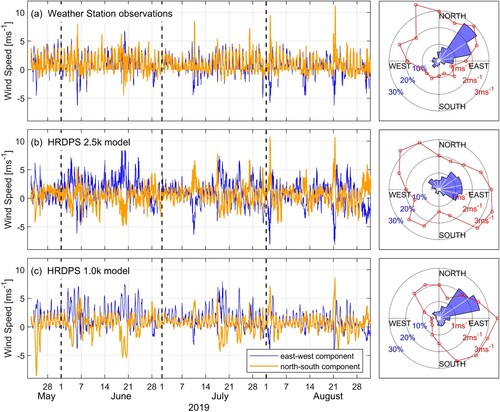
Acknowledging the fact that this farm is located off the northeast corner of Saranac Island and may not accurately capture winds from some directions, there are notable differences between the three wind time series. For example, whereas the two components of the observed winds are generally of comparable magnitude, except during a few storm events, the east–west component (blue) for the two model winds generally dominates. Also, while the strong northwestward winds observed on 1–2 August and 21 August were reproduced with the 2.5 km model, they were underestimated by the 1.0 km model.

Wind roses computed for each vector time series also reveal notable differences. Forty-six percent of the observed winds were toward the northeast and east-northeast directions that approximately align with the channel, with corresponding average speeds of 2.9 and 2.5 m s⁻¹, respectively. No winds in any other of the sixteen wind-rose compass directions arose more than ten percent of the time, though some of their average speeds were larger than 2.5 m s⁻¹. The wind rose for the 2.5 km HRDPS model had the largest percentage of winds toward the east and east-northeast with several average speeds larger than 3.0 m s⁻¹ and an average speed polygon that is seen to be quite different than that observed. Finally, although the wind rose for the 1.0 km HRDPS winds has a directional polygon that is close to that observed, it is not clear that the associated average speed polygon is any closer to that observed than the 2.5 km model winds. Those differences aside, all time series displayed regular daily sea breeze signals that Fast Fourier Transform analyses confirm are in reasonable agreement. Specifically, whereas the observed sea breeze had an average amplitude and direction (toward) of 1.35 m s⁻¹ and 40° counter-clockwise from east, respectively, corresponding values for the 2.5 and 1.0 km HRDPS models were 1.38 m s⁻¹ and 39°, and 1.44 m s⁻¹ and 31°, respectively.

f Freshwater Forcing

As discussed in Appendix A, there are numerous assumptions and approximations related to the freshwater forcing that could either be eliminated or made more accurate with additional observations and/or the development of a hydrology model. Such improvements would require collaboration with Water Survey of Canada (ECCC), PacFish, and hydrologists/modellers from the provincial government or academia.

g Numerical Approximations in the Model

The numerical approximations to each of the terms in the associated hydrodynamic and transport-diffusion partial differential equations that are solved by FVCOM has certainly introduced some inaccuracies. Of course, this is an issue with all numerical models, and it is important to determine which approximations (e.g. to the lateral diffusion term) are causing significant errors, which can be reduced by changes to the numerical approximations, grid, bathymetry, or forcing fields.

h Observational Datasets

Finally, not only can there be problems with the forcing fields and model approximations but as was pointed out with the Fortune1 ADCP values, they may also exist with the observations. Fig. 11 suggests that both issues were present with the HRDPS and observed winds from the Laperouse buoy (C46206 on Fig. 1) during our model simulation period. The HRDPS winds are seen to have a gap of a few days starting 14 April that has since been corrected in the most recent ECCC master archive. (Our version was downloaded earlier.) This did not pose a problem for the simulation as FVCOM simply performs a linear interpolation to obtain values at missing time steps. A scan of the observed winds over this gap shows that although that interpolation would have provided reasonable values, it might explain some of the underestimated E01 along-shelf flows seen in Fig. 7(c). Of more concern, is the fact that the ratio of observed to model wind speeds drops well below 1.0 in late May and remains low for the remainder of the simulation period. This suggests a problem with the anemometer, which is substantiated with a longer time series plot (not shown) where the ratio abruptly returns to around 1.0 in September, likely after the faulty instrument was fixed. Buoy minus HRDPS directional differences show an average discrepancy of approximately −15° (dashed line) for most of the time series and this is confirmed with the associated wind roses which indicate the predominant model winds are on average, rotated clockwise by about 15°. To determine the extent to which such a bias would affect our FVCOM results, a new simulation was conducted (albeit in 2019 with slight modifications of the grid shown in Fig. 2) with all HRDPS winds rotated counter-clockwise so the Laperouse wind rose aligned with the observed. The results showed very little difference in the along-shelf velocity profiles at E01 and virtually identical values in an analogous plot of the along-inlet velocity profiles at MUC1 (Fig. 1) in Muchalat Inlet. Further discussion of the results of this new simulation are beyond the scope of the present study. However, it can be concluded that the model is relatively insensitive small rotations in the forcing winds.

Further comparisons are required to determine if the accuracy of HRDPS model winds at Saranac Island and the Laperouse buoy are representative of those elsewhere in the FVCOM domain. However, the foregoing comparisons do indicate that switching the atmospheric forcing from the 2.5 km HRDPS model to the 1.0 km model will not fully correct inaccuracies in all inlets. To garner further improvements, either a finer resolution atmospheric model (perhaps one that has two-way coupling with the ocean), and/or one that assimilates observations, may be required.

5 Summary

The foregoing presentation has described the development and evaluation of an ocean circulation model for the central west coast of Vancouver Island with particular attention to the numerous inlets. In order to better represent the complicated coastline, an unstructured triangular grid with resolution as small as 60 m was used to cover the domain horizontally and terrain-following coordinates were employed in the vertical direction. The period of 1 March to 31 July 2016 was simulated using the numerical model FVCOM with initial conditions and outer boundary forcing provided by the larger-domain CIOPS-W model, atmospheric forcing interpolated from the 2.5 km version of HRDPS, and freshwater discharge and temperature taken either from Water Survey of Canada (WSC) or PacFish observations, or by estimating those values based on watershed area ratios or other watersheds with similar characteristics. Model results were evaluated through comparisons with a combination of ADCP, tide gauge, Microcat CTD, and salmon farm observations.

The model results were generally in good agreement with observations of (i) tidal elevations and currents everywhere throughout the model domain, and (ii) subtidal currents and temperature and salinity along the shelf. However, it fared poorly in inlets where (i) the tidal currents were relatively weak and not the dominant source of mixing and/or (ii) steep bathymetry necessitated excessive smoothing. Specifically, Figs. 6, 8b, and B5 demonstrated that the model captured the low-pass filtered currents, tidal currents, and bottom temperature and salinity at the TOF1 mooring reasonably well, while Figs. 7, 8c, and B6 showed this was not the case at the ZUC1 mooring. An extensive discussion of sources of these and other inaccuracies, and the changes needed to overcome them, was presented in Section 4. Differences in the dominant dynamics (e.g. tides at mooring TOF1 versus sea breeze at mooring ZUC1) and the modelling adjustments needed to simulate them emphasize the heterogeneity of these glacially-modified seascapes. The information gained through this modelling exercise will hopefully be of use for other nearshore ocean models in regions with fjords, inlets, and channels.

Despite the foregoing challenges, this model is the first fully baroclinic, high-resolution representation of all inlets in the Clayoquot Sound, Nootka Sound and Esperanza Inlet regions. Regarding the initial goal of this study, namely developing a circulation model that can be used to assist in informing decisions on the siting and management of fish farms, progress on two fronts can be noted. The first is that velocities from the FVCOM simulation have already been combined with a particle tracking model to study hydrodynamic connectivity between finfish aquaculture facilities along the west coast of Vancouver Island (DFO, 2022). The second is that, as part of an ongoing project to study hypoxia in this region, a modified version of the foregoing circulation model has been coupled to a biogeochemical model (Bianucci et al., 2018; Khangaonkar et al., 2012). As seen in Fig. 9, the relaxation of strong upwelling on the shelf can induce density intrusions, which can carry low oxygen and nutrient rich water into inlets. This physical mechanism, along with the fact that nutrient rich water can lead to plankton blooms that further deplete oxygen, are likely causes of low oxygen in regions with salmon farms.

Another source of low oxygen in many coastal inlets is the daily sea breeze, as illustrated in Fig. 10 for Saranac Island. Although the present FVCOM simulation is limited in capturing the effects of this wind due to the 2.5 km resolution of the HRDPS model, near surface ADCP measurements (not shown) at mooring MUC1 (Fig. 1) have daily oscillations that are larger than those expected from the diurnal tides. These were reproduced with a secondary FVCOM simulation that, based on observations at a nearby weather station, artificially increased the HRDPS daily winds by a factor of 2.5 in the Muchalat Inlet. In particular, animations of the model near-surface temperature and salinity suggested these oscillations arose when the freshwater lens, generated primarily by the Gold River discharge, was simply pushed back-and-forth (condensed eastward and then relaxing westward) with the daily sea breeze. As farm observations show similar oscillations in the dissolved oxygen at 5 m depth (Liam Peck, personal communication), it will be important to better understand the role that these winds and the oxygen biogeochemistry play in generating low oxygen events at salmon farms. In short, both large-scale (the relaxation of upwelling along the shelf) and small-scale (daily sea breeze) events were partially captured (admittedly with limited accuracy in some, but not all, inlets) by the FVCOM simulation. Improvements along the lines of those described in Section 4 are ongoing and will be reported in future manuscripts.

Acknowledgements

We wish to acknowledge the Aquaculture Collaborative Research and Development Program (ACRDP, DFO) for partial financial support; David Spears, Tom Juhasz, Lucius Perrault, and crews of the J.P Tully and Vector for ADCP deployment and recovery; Cermaq Canada and Grieg Seafood for temperature and salinity observations, useful discussions, and partial financial support (through ACRDP); Michael Dunphy for assistance in running and debugging FVCOM; John Morrison for evaluating some of the HRDPS winds; Neil Goeller, Diana McHugh, Philip Pereboom, and Ian Giesbrecht for assistance in prescribing river discharge and temperature; Anne Ballantyne for providing tide gauge harmonics; Hauke Blanken for providing CIOPS-W plots at the E01 mooring location and the 1.0 km HRDPS wind fields; and the reviewers of earlier versions of the manuscript for their thorough reading and numerous constructive comments.

Disclosure statement

No potential conflict of interest was reported by the author(s).

Appendices

Appendix A: freshwater discharge forcing

In this study, the discharges of twenty-nine rivers (Fig. A1) provided freshwater input along the portion of the western Vancouver Island coast that lies within the model domain. As only five of these rivers were gauged by Water Survey of Canada (WSC, https://wateroffice.ec.gc.ca/) in 2016, discharges for the others had to be estimated and this was done with a variety of approaches, such as scaling by the ratio of the area of an ungauged watershed to the area of another that was gauged. In such cases, watershed areas were either taken from http://viu.maps.arcgis.com/apps/webappviewer/index.html?id = cbcac09d75bc4574baa0d277ea9d8896 or estimated from a topographic map. Although this information may be revised in the future, to our knowledge it was the best available at the time. FVCOM also requires temperature and salinity for these discharges, and again, as observations were sparse, most of these values also had to be estimated. This appendix provides details on the specific calculations.

Fig. A2 shows daily discharges for the five rivers (Gold, Zeballos, Sproat, Sarita, Tofino) that were gauged by WSC for the period of 1 March to 16 July 2016. Estimated values for the Bedwell, Nahmint, Burman, and Somass Rivers are also shown, as in each case those estimates could be made from discharge or stage (elevation) observations on those rivers for the same, or an earlier time period. Specific details are as follows.

1. Burman River discharges were estimated (Neil Goeller, personal communication) by inserting stage measurements provided in the PacFish Hydromet data archive (http://pacfish.ca/wcviweather/) over the period of August 2014 to November 2017 into a stage-discharge curve that was created from previously collected data (Diana McHugh and Philip Pereboom, personal communication).

2. WSC measured daily Bedwell River discharges for the period of April 1990 to March 1999 at a location upstream of the confluence with the Ursus River, its major tributary, and measured Ursus River discharges over the period of 1 January to 6 October 1998, but at a location well upstream of its confluence with the Bedwell. Linearly regressing the Ursus flows against those for the Bedwell over the common time period yielded a correlation coefficient (R²) of 0.81 and a regression coefficient of 3.16. As the Bedwell watershed areas is approximately 1.53 larger than that for the Ursus (Table A1), this larger regression coefficient is probably a reflection of the flow at the Ursus gauge not accounting for the entire watershed (assuming uniform precipitation over both watersheds). So, the watershed ratio has been used to scale up the Bedwell flows. In order to estimate the Bedwell flows for 2016, they in turn were linearly regressed against 1990–1999 values from the Gold River and 1995–1999 flows from Tofino Creek (which only started in May 1995) to determine which provided the better fit. Based on the Giesbrecht et al. (2022) studies of the pluvial versus nivial-glacial runoff characteristics of many BC rivers, it was expected the Gold would provide a better fit. However, limiting observations to between 1 March and 31 July, R² for the Bedwell versus Gold and Bedwell versus Tofino regressions were 0.52 and 0.68 respectively. So, the Tofino was used instead. With a scaling coefficient of 1.67 to account for the Ursus River, the Bedwell estimated discharge is shown in Fig. A2.

3. WSC measured Nahmint River discharges for the period of August 1924 to April 1931. Of the five rivers for which WSC has 2016 observations, only the Sproat River had historical observations going that far back so it had to be used for the linear regression. In this case, the R² value was 0.55 and the Nahmint discharges were 0.6168 those of the Sproat.

4. Finally, WSC only measured Somass River discharges for the period of October 1957 to December 2002 so its 2016 values were estimated by establishing a linear relationship with the Sproat River, which becomes the Somass after merging with the Stamp River. In this case, linear regression yielded an R² of 0.91 with the Somass discharges being 2.8716 those of the Sproat. These results are similar to those computed by Hyatt et al. (2015).

The relative smoothness of the Sproat and Somass discharges reflect the fact that those flows are largely controlled by weirs on Sproat Lake and Great Central Lake. Discharges for the remaining twenty-one rivers were estimated based on the relative area of their watershed to the area of a watershed whose river discharge was measured or estimated, and whose flow characteristics were deemed to be similar (Giesbrecht et al., 2022). Details are summarized in Table A1.

PacFish has also measured hourly water temperature near several river mouths around the Vancouver Island coast. Those within, or near, our model domain and having observations over the period of 1 March to 31 July 2016, were the Sproat, Stamp, Bedwell, and Kaouk Rivers. PacFish observations were also available for the Nahmint River starting on 5 April 2016, and Diana McHugh and Philip Pereboom (personal communication) provided observations for the Burman River starting 1 March. Though some of the hourly time series in the later months have sub-daily oscillations that are presumably due to atmospheric and solar heating/cooling, our ocean circulation model only requires daily values so averages were taken. These are plotted in Fig. A3. As expected, all temperature time series show generally increasing values from spring to summer. The Burman, Bedwell, and Kaouk Rivers have smaller increases because they originate at higher (and cooler) elevations while the Sproat, Stamp, and Nahmint flow from relatively large lakes (Sproat, Great Central, and Nahmint, respectively) whose surface waters are more responsive to atmospheric heat flux warming.

The basis of temperature estimates for the rivers without measurements is summarized in Table A1. In most cases, they were the same as those for a nearby measured river. The Somass temperature was a weighted combination of the Sproat and Stamp values with the weights proportional to their watershed areas. As the Kennedy River drains a large lake, its temperature was assigned the same values as the Sproat River, whose drainage is similar. Finally, as the Nahmint observations did not start until 5 April, its values from 1 March were set to those for the relatively close Stamp River.

Discharge salinity can be trickier to assign. As the model grid does not extend up each river channel to the point where there is no mixing with ocean water, setting discharge salinity to zero can lead to values that are too fresh further down the inlet (Foreman et al., 2012). Foreman et al. (2015) adopted the approach of assigning discharge salinity to mid-month climatological averages in the top 5 ms of the water column at grid nodes nearest the river mouths but this often produced values that were too salty when compared with in-situ observations further down the inlets. Here we employ a FVCOM input parameter setting wherein “the salinity or temperature at discharge nodes is calculated using the mass conservative salinity or temperature equation” (Chen et al., 2006b). As discussed in Appendix B, this provided reasonable agreement with nearby fish farm observations.

Fig. A1 Locations of the rivers whose volume discharges, temperature, and salinity were used in the model forcing.

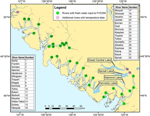
Fig. A2 Observed and estimated river discharges (m s⁻³) for the period of 1 March to 31 July 2016. WSC observations are shown in the upper panel while estimated values are shown in the lower panel. A log scale has been used to help differentiate small values.

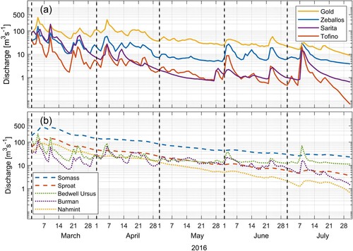
Fig. A3 Daily averaged river temperature (°C), 1 March to 31 July 2016.

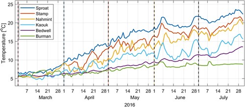
Table A1. Summary of freshwater discharge details used in the March-July 2016 model simulation.

	Name	Discharge (m s^−3)	Temperature (°C)	Watershed area (km^2)
1	Sarita River	WSC	E (Nahmint)	161.54
2	Franklin River	WR (Sarita)	E (Nahmint)	136.58
3	Somass River	HR (Sproat)	PF (Sproat & Stamp)	1297.39 (Sproat, 350.96; Stamp, 613.72)
4	Nahmint River	HR (Sproat)	PF (& E Kaouk)	192.29
5	Henderson River	WR (Sarita)	E (Nahmint)	141.86
6	Effingham River	WR (Sarita)	E (Nahmint)	59.82
7	Toquart River	WR (Sarita)	E (Nahmint)	103.74
8	Maggie River	WR (Sarita)	E (Nahmint)	59.77
9	Kennedy River	WR (Somass)	E (Sproat)	551.16
10	Tofino Creek	WSC	E (Bedwell)	37.26
11	Bulson River	WR (Bedwell)	E (Bedwell)	82.36
12	Bedwell River + Ursus Creek	HR (Tofino)	PF	112.36 + 73.64
13	Moyeha River	WR (Bedwell)	E (Bedwell)	181.52
14	Watta + Talbot Creeks	WR (Bedwell)	E (Bedwell)	40.62 + 244.43
15	Sydney River	WR (Tofino)	E (Bedwell)	58.21
16	Hesquiat River	WR (Tofino)	E (Bedwell)	30.0 (estimated)
17	Mooyah River	WR (Zeballos)	E (Burman)	37.87
18	Silverado River	WR (Zeballos)	E (Burman)	40.0 (estimated)
19	Houston River	WR (Zeballos)	E (Burman)	50.33
20	Jacklah River	WR (Zeballos)	E (Burman)	48.40
21	Burman River	PBS	PBS	242.36
22	Gold River	WSC	E (Burman)	991.37
23	McCurdy Creek	WR (Zeballos)	E (Burman)	69.98
24	Kleeptee River	WR (Zeballos)	E (Burman)	52.64
25	Tlupana River	WR (Zeballos)	E (Burman)	106.42
26	Nuchaltlitz River	WR (Zeballos)	E (Kaouk)	40.0 (estimated)
27	Tahsis River	WR (Zeballos)	E (Kaouk)	76.52
28	Zeballos River	WSC	E (Kaouk)	168.79
29	Espinosa River	WR (Zeballos)	E (Kaouk)	27.09

See Fig. A1 for river locations. Legend: WSC = Water Survey of Canada observation, PF = PacFish observation, HR = estimate based on historical WSC relationship, WR = watershed ratio, PBS = Pacific Biological Station (personal communication, Philip Pereboom and Diana McHugh) observation, E = estimate based on PF or PBS observation. Except where denoted as “estimated”, watershed areas were taken from http://viu.maps.arcgis.com/apps/webappviewer/index.html?id = cbcac09d75bc4574baa0d277ea9d8896. The Hesquiat, Silverado, and Nuchaltlitz areas were not available on this site and were estimated from a topographic map.

Appendix B: evaluation of model salinity and temperature

B1 Fish farms

Temperature, salinity, and oxygen observations were taken over the first four months of the model simulation period by Cermaq Canada at eleven farms in the Clayoquot region and over the complete five-month simulation period by Grieg Seafood at five farms in the Nootka and Esperanza regions. (See Fig. B1 for farm locations). Up to three measurements were taken each day (none at night) at depths 1, 5, 10, and 15 m; however, gaps were numerous and the specific sampling times were not consistent so that some tidal and daily sea-breeze aliasing can be expected. In addition, as all measurements were taken and recorded manually; there were some errors that had to be corrected by de-spiking time series plots. Although the salinity was measured in parts-per-thousand (ppt), the precision of the measurement instrument was only one decimal place. So, we assumed the ppt values were equivalent to absolute.

Fig. B2 illustrates the salinity and temperature time series at the Williamson Passage farm in Muchalat Inlet. High variability in the salinity at 1 m depth is due to a combination of freshwater runoff events from nearby (Mooyah & Kleeptee; see Fig. A1) and remote (Gold and Burman) rivers and wind mixing from storms. The extent to which this variability has decreased at 5, 10 and 15 m also indicates the changing thickness of the freshwater lens, although the numerous salinity values of 30 at 10 and 15 m depth also indicate questionable values in the dataset. The 1 m temperature is seen to have an increasing trend over March to July, with variability likely due to intermittent warmer/cooler and sunnier/cloudier days. Note that the 1 m values are colder than those below up to approximately 1 April and then warmer thereafter; a reflection of warming air temperature and increased solar radiation. Interestingly, the 5 m temperature from 1 May onward shows more variability than those at 1 m, while the 10 and 15 m values are very close and generally show the least variation. Although oscillations in the 5 m temperature may be due to internal waves or daily sea breeze interactions with the surface thermocline, aliasing and precision of the present measurements complicate further investigation.

Nevertheless, these farm observations provide an excellent data set to evaluate the accuracy of model salinity and temperature over the top 15 m of the water column in many inlets. Table B1 shows root mean square and average differences at sixteen farms and two depths, 1, and 10 m. The model salinity and temperature were taken from the node nearest the farm location and interpolated linearly in both time and depth to match the observations. To illustrate the nature of these differences, Fig. B3 shows model and observed salinity and temperature time series at 1 m depth at the Bare Bluff farm in Bedwell Sound (Fig. 1). Like those in Fig. B2, the observed salinity has considerable variability with sharp downward spikes arising from large discharge events in the nearby Bedwell River. The model salinity is also seen to have downward spikes although they do not necessarily correspond in time, nor do they reach the same low values as those observed. The relatively poor agreement between these two salinity time series (correlation 0.62) is at least partially because the Bedwell River volume discharges were not measured directly but rather inferred from those for the Tofino Creek (see Appendix A for details). The modelled and observed temperature are in much better agreement with a correlation of 0.94 between the two-time series. The Bedwell River temperature used in the model forcing were taken from PacFish measurements (Appendix A) and, in light of the high correlation, must be a major influence on the near-surface farm temperature further down inlet.

Table B1. Root mean square and average differences (RMS, avdif) between model and farm salinity (S, absolute) and temperature (T, °C) at two depths over the period of 1 March to 31 July 2016. Average differences are model minus observed.

Farm name	# obs.	RMS S, 1 m	RMS T, 1 m	RMS S, 10 m	RMS T, 10 m	avdif S, 1 m	avdif T, 1 m	avdif S, 10 m	avdif T, 10 m	Region
Fortune	230	3.3	1.2	3.1	1.1	2.3	−0.5	2.3	−0.7	Clayoquot
Plover	236	2.1	2.0	1.5	1.7	1.2	1.1	0.9	0.9
Bedwell	217	2.8	1.6	2.6	1.0	2.1	0.8	1.9	0.4
Bare Bluff	238	3.1	1.4	2.3	1.5	1.0	0.7	1.1	1.0
Westside	238	2.5	1.6	2.5	1.2	1.4	0.9	1.9	0.5
Mussel Rock	238	4.6	1.4	2.4	1.7	3.1	1.0	1.3	1.3
Saranac	234	2.8	2.7	2.4	2.5	1.7	2.1	1.4	2.0
Bawden	361	3.3	1.3	1.9	0.8	0.9	0.1	0.2	−0.4
Binns	353	3.6	1.6	1.5	1.0	1.4	0.1	−0.2	0.2
Ross	222	3.2	1.1	1.6	0.6	1.9	0.2	0.5	−0.3
Millar	229	2.5	1.5	1.9	0.8	−0.8	0.7	−1.4	−0.5
Williamson	306	8.5	2.2	1.6	1.0	7.2	−1.7	0.2	−0.7	Nootka
Atrevida	301	8.6	1.8	1.5	1.3	7.3	−1.2	−0.2	−1.0
Concepcion	306	7.8	1.8	1.8	1.0	6.9	−1.3	1.0	−0.7
Esperanza	302	4.5	1.4	2.1	0.9	2.0	−0.8	−1.4	−0.1	Esperanza
Steamer	299	3.0	1.1	2.7	0.8	0.6	−0.4	−2.2	0.0
Average	269	4.1	1.6	2.1	1.2	2.5	0.1	0.5	0.1

However, although the model temperatures are slightly lower than those observed up until 15 April, they are higher after that date and on average, 0.8°C larger over the entire time series. In fact, with the exception of Fortune, all farms in the Clayoquot Sound region have model versus observed temperature plots that are similar to those in Fig. B3 and average model temperature that are warmer than observed. The fact that the Nootka and Esperanza farm model temperature are, on average, cooler than those observed (Table B1) suggests that either their nearby river temperature is too cold, or the spring and early summer heat flux has been over-estimated in the Clayoquot region but not further north. Further investigation into the accuracy of the HRDPS variables used in the heat flux calculation is clearly warranted but will not be pursued here.

With the exception of the Millar farm, the model salinity at 1 m depth is, on average, too salty over the simulation period. Further research is needed to determine the reasons behind this bias including the extent of vertical mixing and the manner in which vertical profiles of the water properties and discharge are specified at the river mouths.

With only a few exceptions, the RMS salinity and temperature differences at 10 m are smaller (and thus more accurate) than those at 1 m. Average salinity and temperature RMS differences over the 16 farms at 15 m depth are very close to those at 10 m while those at 5 m are between those given in Table B1 for 1 and 10 m. So in general, over the top 15 m of the water column the accuracy of model salinity and temperature increases with depth.

The much larger salinity differences at Atrevida, Concepcion, and Williamson are particularly note-worthy and warrant further attention. These three farms are located within 5 km of each other at the seaward end of Muchalat Inlet. Their large 1 m salinity discrepancies suggest that (i) the model freshwater plume originating with larger discharges from the Gold and Burman Rivers at the head of the inlet experiences too much mixing as it moves eastward down the inlet, (ii) there are local freshwater sources near these farms that have been under-estimated (e.g. Mooyah and Kleeptee Rivers) or not included in the model, or (iii) a combination of both. In an effort to improve the representation of the freshwater plume, tests were carried out with hybrid vertical coordinates and constant near-surface thicknesses. However, two hybrid choices (one with six surface layers of thickness 0.25, 0.5, 0.75, 1, 1, and 1 m respectively; and the other with ten surface layers each with 2 m thickness) showed that this was not the case. In both instances the average salinity error at 1 m depth was larger than with the sigma coordinate choice whose results are summarized in Table B1. This issue was discussed further in Section 4.

A further suggestion of too much vertical mixing can be seen in the salinity time series at the Muchalat North farm (Fig. B4). Although the farm was not operational during the FVCOM simulation period of March-July 2016, observations were made in 2017 and as seen in Fig. B3, there is a strong negative correlation between the Gold River discharge and farm salinity at 1 m; for example, the salinity starts decreasing when the river discharge starts increasing on 11 March 2017. While the 2016 discharge is different than in 2017, it would still be reasonable to expect the salinity to decrease rapidly following a peak discharge and have values comparable to those seen after the 2017 peak. Although the 2016 model salinity does decrease as the freshwater plume reaches the farm down inlet, it does not decrease to the values observed in 2017 when the peak discharge was smaller. So as hypothesized earlier, it seems that either the model is not accurately preserving the surface freshwater plume as it moves westward down Muchalat Inlet, or it is missing some local sources of freshwater.

B2 Microcats

Time series of temperature and salinity were also collected by Microcat CTDs moored at the same depths as those for the ADCP instruments. Fig. B5 shows near bottom temperature and salinity observed (half-hourly) and model (hourly) time series at the E01 mooring. In this case, the observations are at 90 m while the model values are at 82 m, halfway down the bottom layer. The respective time series are seen to be in good agreement with RMS differences in the hourly temperature and salinity being 0.4°C and 0.3, respectively. Daily CIOPS-W temperature and salinity at 97 m depth that were interpolated to the boundary node nearest to E01 (approximately 16.6 km away) show reasonable agreement with their FVCOM counterparts. This is to be expected given that model temperature and salinity along the outer boundary are nudged back to the CIOPS-W values with a time scale of two hours. The higher CIOPS-W salinity seen in March is likely because this boundary node is closer to the shelf break than E01 and thus less influenced by freshwater discharges along the coast. Note that whereas the observed salinity was sampled every half-hour and, therefore, capable of capturing tidal oscillations, the CIOPS-W salinity that was used to force FVCOM was only daily (that was the storage frequency) so it aliased the tidal signals. The fact that the FVCOM time series includes some oscillations suggests that the model dynamics have generated some baroclinic tides.

Both model and Microcat observations display high-frequency variability at 32 m depth at TOF1 (Fig. B6). Tidal oscillations are clearly evident in all time series and close-up plots over shorter time periods (not shown) reveal that salinity has twice daily decreases that arise when the strong semi-diurnal ebb tide brings fresher water from further up the inlet past the mooring. A spring-neap cycle consistent with that seen earlier for the low-pass filtered along-channel velocities (Fig. 8) is also evident. For example, bottom salinity is seen to increase during the neap tides around 17 and 31 March and 16 and 30 April, when there is less tidal mixing and more saline bottom water enters from the shelf, and fresher water escapes seaward near the surface. The mid-June drop in observed salinity that lasts about a week, has small tidal oscillations, and then quickly increases back up to the pre-decrease levels, is mysterious. As the observed temperature does not show similar changes, further investigation into the data processing is required but beyond the scope of this study. The mid-April divergence of model and observed average temperatures can be explained by the model bathymetric smoothing. The model depth at TOF1 is 26.3 m, shallower than depth of the Microcat and ADCP (Fig. 8). Thus, the model temperatures will warm sooner, as the seasonal air temperatures increase and their affect spreads down the water column, and they will remain warmer until the end of the simulation.

The RMS model minus observed temperature differences are 1.0° C and 0.7 respectively. On average, the model temperature is 0.7° C warmer, and the salinity is essentially the same as that observed. The warmer temperature is consistent with findings described earlier at most of the Clayoquot farms with the differences attributed to a combination of both over-estimated heat fluxes and too much vertical mixing, as was seen at ZUC1. Note that a portion of the RMS errors will be due to the tides; i.e. inaccuracies in the model constituent magnitudes and phases and the fact that the model only includes eight constituents and the nonlinear harmonics they generate, as opposed to the much larger number that exist naturally and are represented in the observations.

Finally, Fig. B7 shows observed and model values at the bottom ZUC1 mooring over the period of 1 March to 12 July 2016. (Note there is slight difference in “bottom” as the observations are at 184 m while the model values lie halfway down the bottom layer, which in this case is 168 m.) The 9–10 May density intrusion, which appeared as a sharp speed increase in the velocity profiles (Fig. 9), now appears in the observations as an abrupt jump with sharp increases and decreases in the salinity and temperature respectively, consistent with a front of cooler, more saline water moving past the mooring. The model time series shows increases and decreases persisting over a longer period of time (from approximately 25 April to 10 May) and larger in magnitude than those observed. Thus, they are a more gradual response to the upwelling conditions that started on the shelf around 25 April. It is also noteworthy that both model time series display much more variability than the observations, which are relatively flat before and after the jumps. In fact, while the model temperature starts in reasonable agreement with their observed counterparts at approximately 9.0°C, they rise rather quickly to attain a maximum of about 10.7°C in late April and only decrease to, and oscillate about, a mean of approximately 10.2°C after 10 May, which is still about 1.2°C larger than the observations. The model salinity also starts in reasonable agreement with the observations but decreases quickly and remains consistently fresher over the model simulation, only rising to within 1.0 in absolute units after 10 May. Both the diffused density front produced by the model and the rapid changes in the initial model temperature and salinity suggest too much vertical mixing bringing warmer and fresher water from up-inlet. (This issue was discussed in Section 4.) RMS temperature and salinity differences between the model and observed time series are 1.2 °C and 1.4, respectively.

The ZUC1 mooring also had a Microcat CTD at 40 m depth and as with the bottom instrument (184 m), it recorded (not shown) a sharp drop in temperature of approximately 0.75°C on 10 May. RMS temperature and salinity differences between hourly observed and model values at 40 m are considerably smaller, namely 0.7 °C and 0.8, respectively. Similarly, the RMS differences in temperature and salinity between the model and the relatively close Atrevida, Concepcion, and Williamson farms at 15 m depth are also smaller, approximately 1.1°C and 1.3 absolute. Although the model accuracy improves with depth over the top 40 m in this region, it deteriorates further down the water column.

Fig. B1 Locations of salmon farms used in model temperature and salinity evaluations.

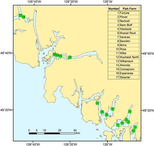
Fig. B2 Observed salinity and temperature at the Williamson Passage farm over the period of 1 March to 31 July 2016.

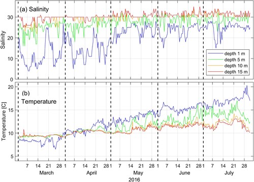
Fig. B3 Observed and modelled salinity (absolute) and temperature (°C) at 1 m depth at the Bare Bluff farm in Bedwell Sound, along with model values interpolated to the same time and depth.

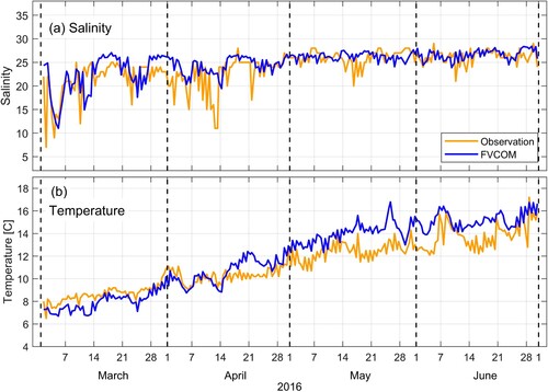
Fig. B4 Model March–May 2016 (a) and observed March–May 2017 (b) salinity at the Muchalat North farm along with corresponding daily discharges for the Gold River.

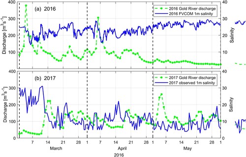
Fig. B5 Near-bottom, half-hourly observed (Microcat) and hourly model (a) absolute salinity and (b) temperature (°C) at E01 for the period of 1 March to 12 July 2016. Analogous daily CIOPS-W values at 97 m depth were interpolated to the boundary node nearest E01 and are also shown.

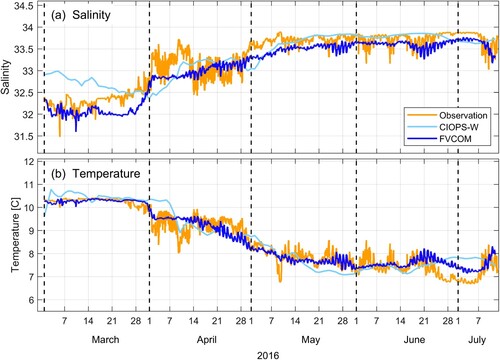
Fig. B6 Bottom observed and model (a) absolute salinity and (b) temperature (°C) at TOF1 for the period of 1 March to 11 July 2016.

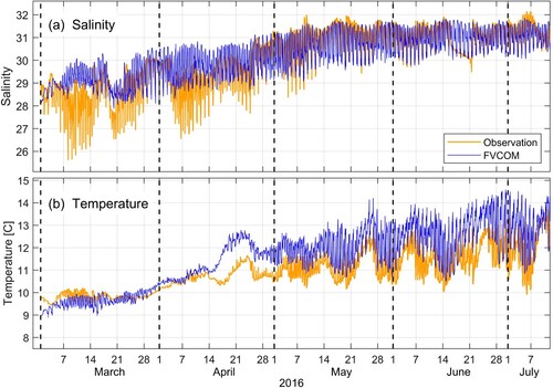
Fig. B7 Model and observed bottom temperature (T, °C) and absolute salinity (S) at the ZUC1 mooring (Fig. 1) for the period of 1 March to 12 July 2016.

References

- Adams, T., Black, K., MacIntyre, C., MacIntyre, I., & Dean, R. (2012). Connectivity modelling and network analysis of sea lice infection in Loch Fyne, west coast of Scotland. Aquaculture Environment Interactions, 3(1), 51–63. https://doi.org/10.3354/aei00052
- Amundrud, T. L., & Murray, A. G. (2009). Modelling sea lice dispersion under varying environmental forcing in a Scottish sea loch. Journal of Fish Diseases, 32(1), 27–44. https://doi.org/10.1111/j.1365-2761.2008.00980.x
- Asplin, L., Boxaspen, K. K., & Sandvik, A. D. (2011). Modelling the distribution and abundance of planktonic larval stages of Lepeophtheirus salmonis in Norway. In S. Lice (Ed.), An integrated approach to understanding parasite abundance and distribution (pp. 31–50). Wiley-Blackwell. https://doi.org/10.1002/9780470961568
- Bianucci, L., Long, W., Khangaonkar, T., Pelletier, G., Ahmed, A., Mohamedali, T., Roberts, M., & Figueroa-Kaminsky, C. (2018). Sensitivity of the regional ocean acidification and carbonate system in Puget Sound to ocean and freshwater inputs. Elementa: Science of the Anthropocene, 6, 22. https://doi.org/10.1525/elementa.151
- Bond, N. A., Cronin, M. F., Freeland, H., & Mantua, N. (2015). Causes and impacts of the 2014 warm anomaly in the NE Pacific. Geophysical Research Letters, 42, 3414–3420. https://doi.org/10.1002/2015GL063306
- Burchard, H., Bolding, K., & Villareal, M. R. (1999). GOTM—a general ocean turbulence model. Theory, applications and test cases. Technical Report EUR 18745 EN, European Commission.
- Chang, B. D., Page, F. H., Losier, R. J., Lawton, P., Singh, R., & Greenberg, D. A. (2007). Evaluation of bay management area scenarios for the southwestern New Brunswick salmon aquaculture industry. Aquaculture Collaborative Research and Development Program final project report. Canadian Technical Report of Fisheries and Aquatic Sciences, 2722, 1–69.
- Chen, C., Beardsley, R. C., & Cowles, G. (2006a). An unstructured grid, finite-volume coastal ocean model (FVCOM) system. Oceanography Special Issue on “Advances in Computational Oceanography”, 19(1), 78–89. https://doi.org/10.1016/j.ocemod.2009.01.007
- Chen, C., Beardsley, R. C., & Cowles, G. (2006b). An unstructured grid, finite-volume coastal ocean model: FVCOM user manual. http://fvcom.smast.umassd.edu/FVCOM/index.html
- Chen, C., Beardsley, R. C., Cowles, G., Qi, J., Lai, Z., Gao, G., Stuebe, D., Xu, Q., Xue, P., Ge, J., Ji, R., Hu, S., Tian, R., Huang, H., Wu, L., & Lin, H. (2011). An unstructured grid, finite-volume coastal ocean model. FVCOM user manual (3rd ed.). Massachusetts Institute of Technology. 315 p.
- Chen, C., Liu, H., & Beardsley, R. C. (2003). An unstructured grid, finite-volume, three-dimensional, primitive equations ocean model: Application to coastal ocean and estuaries. Journal of Atmospheric and Oceanic Technology, 20(1), 159–186. https://doi.org/10.1175/1520-0426(2003)020<0159:AUGFVT>2.0.CO;2
- Chen, C., Xu, Q., Houghton, R., & Beardsley, R. C. (2008). A model-dye comparison experiment in the tidal mixing front zone on the southern flank of Georges Bank. Journal of Geophysical Research, 113(C2), C02005. https://doi.org/10.1029/2007JC004106
- Crawford, W. R., & Thomson, R. E. (1984). Diurnal-period continental shelf waves along Vancouver Island: A comparison of observations with theoretical models. Journal of Physical Oceanography, 14(10), 1629–1646. https://doi.org/10.1175/1520-0485(1984)014<1629:DPCSWA>2.0.CO;2
- Cummins, P. F., Masson, D., & Foreman, M. G. G. (2000). Stratification and mean flow effects on diurnal tidal currents off Vancouver Island. Journal of Physical Oceanography, 30(1), 15–30. https://doi.org/10.1175/1520-0485(2000)030<0015:SAMFEO>2.0.CO;2
- Davies, S. C., Gregr, E. J., Lessard, J., Bartier, P., & Wills, P. (2019). Coastal digital elevation models integrating ocean bathymetry and land topography for marine ecological analyses in Pacific Canadian waters. Canadian Technical Report of Fisheries and Aquatic Sciences, 3321, vi + 38 p.
- DFO. (2022). Hydrodynamic connectivity between Marine Finfish aquaculture facilities in British Columbia: In support of an area based management approach. DFO Canadian Science Advisory Secretariat Science Response. 2021/042.
- Egbert, G. D., & Erofeeva, S. Y. (2002). Efficient inverse modeling of barotropic ocean tides. Journal of Atmospheric and Oceanic Technology, 19(2), 183–204. https://doi.org/10.1175/1520-0426(2002)019<0183:EIMOBO>2.0.CO;2
- Elmoslemany, A., Revie, C., Milligan, B., Stewardson, L., & Vanderstichel, R. (2015). Wild juvenile salmonids in Muchalat Inlet, British Columbia, Canada: Factors associated with sea lice prevalence. Diseases of Aquatic Organisms, 117(2), 107–120. https://doi.org/10.3354/dao02939. PMID:26648103.
- Emery, W. J., & Thomson, R. E. (2014). Data analysis methods in physical oceanography (3rd ed.). Elsevier.
- Engida, Z., Monahan, A., Ianson, D., & Thomson, R. E. (2016). Remote forcing of subsurface currents and temperatures near the northern limit of the California Current System. Journal of Geophysical Research: Oceans, 121(10), 7244–7262. https://doi.org/10.1002/2016JC011880
- Environment and Climate Change Canada. (2015). High resolution deterministic prediction system, online. Retrieved March 6, 2016, from https://weather.gc.ca/grib/grib2_HRDPS_HR_e.html
- Environment and Climate Change Canada. (2016). Water survey of Canada: Hydrometric data. https://wateroffice.ec.gc.ca/index_e.html
- Fairall, C. W., Bradley, E. F., Hare, J. E., Grachev, A. A., & Edson, J. B. (2003). Bulk parameterization of air-sea fluxes: Updates and verification for the COARE algorithm. Journal of Climate, 16(4), 571–591. https://doi.org/10.1175/1520-0442(2003)016<0571:BPOASF>2.0.CO;2
- Flather, R. A. (1988). A numerical model investigation of tides and diurnal-period continental shelf waves along Vancouver Island. Journal of Physical Oceanography, 18(1), 115–139. https://doi.org/10.1175/1520-0485(1988)018<0115:ANMIOT>2.0.CO;2
- Foreman, M. G. G., Callendar, W., MacFadyen, A., Hickey, B. M., Thomson, R. E., & Di Lorenzo, E. (2008). Modeling the generation of the Juan de Fuca Eddy. Journal of Geophysical Research, 113(C3), C03006. https://doi.org/10.1029/2006JC004082
- Foreman, M. G. G., Cherniawsky, J. Y., & Ballantyne, V. A. (2009). Versatile harmonic tidal analysis: Improvements and applications. Journal of Atmospheric and Oceanic Technology, 26(4), 806–817. https://doi.org/10.1175/2008JTECHO615.1
- Foreman, M. G. G., Crawford, W. R., Cherniawsky, J. Y., & Galbraith, J. (2008). Dynamic ocean topography for the Northeast Pacific and its continental margins. Geophysical Research Letters, 35(22), L22606. https://doi.org/10.1029/2008GL035152
- Foreman, M. G. G., Czajko, P., Stucchi, D. J., & Guo, M. (2009). A finite volume model simulation for the Broughton Archipelago, Canada. Ocean Modelling, 30(1), 29–47. https://doi.org/10.1016/j.ocemod.2009.05.009
- Foreman, M. G. G., Guo, M., Garver, K. A., Stucchi, D., Chandler, P., Wan, D., Morrison, J., & Tuele, D. (2015). Modelling infectious hematopoietic necrosis virus dispersion from marine salmon farms in the Discovery Islands, British Columbia, Canada. PLoS ONE, 10(6), e0130951. https://doi.org/10.1371/journal.pone.0130951
- Foreman, M. G. G., & Henry, R. F. (1989). The harmonic analysis of tidal model time series. Advances in Water Resources, 12(3), 109–120. https://doi.org/10.1016/0309-1708(89)90017-1
- Foreman, M. G. G., Stucchi, D. J., Garver, K. A., Tuele, D., Isaac, J., Grime, T., & Guo, M. (2012). A circulation model for the Discovery Islands, British Columbia. Atmosphere-Ocean, 50(3), 301–316. https://doi.org/10.1080/07055900.2012.686900
- Foreman, M. G. G., Sutherland, G., & Cummins, P. F. (2004). M2 Tidal dissipation around Vancouver Island: An inverse approach. Continental Shelf Research, 24(18), 2167–2185. https://doi.org/10.1016/j.csr.2004.07.008
- Foreman, M. G. G., & Thomson, R. E. (1997). Three-dimensional model simulations of tides and buoyancy currents along the west coast of Vancouver Island. Journal of Physical Oceanography, 27(7), 1300–1325. https://doi.org/10.1175/1520-0485(1997)027<1300:TDMSOT>2.0.CO;2
- Foreman, M. G. G., Thomson, R. E., & Smith, C. L. (2000). Seasonal current simulations for the western continental margin of Vancouver Island. Journal of Geophysical Research: Oceans, 105(C8), 19665–19698. https://doi.org/10.1029/2000JC900070
- Freeland, H. J., Crawford, W. R., & Thomson, R. E. (1984). Currents along the Pacific coast of Canada. Atmosphere-Ocean, 22(2), 151–172. https://doi.org/10.1080/07055900.1984.9649191
- Giesbrecht, I. J. W., Tank, S. E., Frazer, G. W., Hood, E., Gonzalez Arriola, S. G., Butman, D. E., D’Amore, D. V., Hutchinson, D., Bidlack, A., & Lertzman, K. P. (2022). Watershed classification predicts streamflow regime and organic carbon dynamics in the Northeast Pacific Coastal Temperate Rainforest. Global Biogeochemical Cycles, 36(2), e2021GB007047. https://doi.org/10.1029/2021GB007047
- Godin, G. (1972). The analysis of tides. University of Toronto Press. 264 pp.
- Griffin, D. A., & LeBlond, P. H. (1990). Estuary/ocean exchange controlled by spring-neap tidal mixing. Estuarine, Coastal and Shelf Science, 30(3), 275–297. https://doi.org/10.1016/0272-7714(90)90052-S
- Haney, R. L. (1991). On the pressure gradient force over steep topography in sigma coordinate ocean models. Journal of Physical Oceanography, 21(4), 610–619. https://doi.org/10.1175/1520-0485(1991)021<0610:OTPGFO>2.0.CO;2
- Hannah, C. G., & Wright, D. G. (1995). Depth dependent analytical and numerical solutions for wind-driven flow in the coastal ocean. In D. R. Lynch, & A. M. Davies (Eds.), Quantitative skill assessment for coastal ocean models, coastal and estuarine studies (pp. 125–152). American Geophysical Union.
- Henry, R. F., & Walters, R. A. (1993). Geometrically based, automatic generator for irregular triangular networks. Communications in Numerical Methods in Engineering, 9(7), 555–566. https://doi.org/10.1002/cnm.1640090703
- Hickey, B. M., Thomson, R. E., Yih, H., & LeBlond, P. H. (1991). Velocity and temperature fluctuations in a buoyancy-driven current off Vancouver Island. Journal of Geophysical Research: Oceans, 96(C6), 10507–10538. https://doi.org/10.1029/90JC02578
- Hsieh, W. W. (1982). On the detection of continental shelf waves. Journal of Physical Oceanography, 12(5), 414–427. https://doi.org/10.1175/1520-0485(1982)012<0414:OTDOCS>2.0.CO;2
- Hyatt, K. D., Stiff, H. W., Stockwell, M. M., Luedke, W., Rankin, D. P., Dobson, D., & Till, J. (2015). A synthesis of adult Sockeye salmon migration and environmental observations for the Somass watershed, 1974-2012. Canadian Technical Report of Fisheries and Aquatic Sciences, 3115, vii + 199 p.
- Jackson, J. M., Johnson, G. C., Dosser, H. V., & Ross, T. (2018). Warming from recent marine heatwave lingers in deep British Columbia fjord. Geophysical Research Letters, 45(18), 9757–9764. https://doi.org/10.1029/2018GL078971
- Khangaonkar, T., Sackmann, B., Long, W., Mohamedali, T., & Roberts, M. (2012). Simulation of annual biogeochemical cycles of nutrient balance, phytoplankton bloom(s), and DO in Puget Sound using an unstructured grid model. Ocean Dynamics, 62(9), 1353–1379. https://doi.org/10.1007/s10236-012-0562-4
- Lu, Y., Li, J., Lei, J., & Hannah, C. (2017). Impacts of model resolution on simulation of meso-scale eddies in the Northeast Pacific Ocean. Satellite Oceanography and Meteorology, 2(2), 328. https://doi.org/10.18063/som.v2i2.328
- Lynch, D. R., & Gray, W. G. (1978). Analytic solutions for computer flow model testing. Journal of the Hydraulics Division, 104(10), 1409–1428. https://doi.org/10.1061/JYCEAJ.0005086
- Masson, D., & Fine, I. (2012). Modeling seasonal to interannual ocean variability of coastal British Columbia. Journal of Geophysical Research: Oceans, 117(C10), C10019. https://doi.org/10.1029/2012JC008151
- Mellor, G. L., Ezer, T., & Oey, L.-Y. (1994). The pressure gradient conundrum of sigma coordinate ocean models. Journal of Atmospheric and Oceanic Technology, 11(4), 1126–1134. https://doi.org/10.1175/1520-0426(1994)011<1126:TPGCOS>2.0.CO;2
- Mellor, G. L., & Yamada, T. (1982). Development of a turbulence closure model for geophysical fluid problems. Reviews of Geophysics, 20(4), 851–875. https://ui.adsabs.harvard.edu/link_gateway/1982RvGSP.20.851M/doi:10.1029/RG020i004p00851
- Michel Lionel, T., Lyard, F., Loren, C., Mathilde, C., Damien, A., Ergane, F., Mei-ling, D., Ramiro, F., Yannice, F., Gerald, D., & Nicolas, P. (2023). The new FES2022 tidal atlas. EGU General Assembly 2023, Vienna, Austria, 24–28 Apr 2023, EGU23-9008. https://doi.org/10.5194/egusphere-egu23-9008
- Navas, J. M., Telfer, T. C., & Ross, L. G. (2011). Application of 3D hydrodynamic and particle tracking models for better environmental management of finfish culture. Continental Shelf Research, 31(6), 675–684. https://doi.org/10.1016/j.csr.2011.01.001
- NEMO Community Ocean Model. https://www.nemo-ocean.eu
- Page, F. H., Losier, R., Haigh, S., Bakker, J., Chang, B. D., McCurdy, P., Beattie, M., Haughn, K., Thorpe, B., Fife, J., Scouten, S., Greenberg, D., Ernst, W., Wong, D., & Bartlett, G. (2015). Transport and dispersal of Sea Lice bath therapeutants from Salmon farm net-pens and well-boats. DFO Canadian Science Advisory Secretariat Research Document, 2015/064. xviii + 148 p.
- Pietrzak, J. D., Jakobson, J. B., Burchard, H., Vested, H. J., & Petersen, H. O. (2002). A three-dimensional hydrostatic model for coastal and ocean modelling using a generalised topography following co-ordinate system. Ocean Modelling, 4(2), 173–205. https://ui.adsabs.harvard.edu/link_gateway/2002OcMod … 4.173P/doi:10.1016/S1463-5003(01)00016-6
- Salama, N. K. G., & Rabe, B. (2013). Developing models for investigating the environmental transmission of disease-causing agents within open-cage salmon aquaculture. Aquaculture Environment Interactions, 4(2), 91–115. https://doi.org/10.3354/aei00077
- Smagorinsky, J. (1963). General circulation experiments with the primitive equations, I. The basic experiment. Monthly Weather Review, 91(3), 99–164. https://doi.org/10.1175/1520-0493(1963)091<0099:GCEWTP>2.3.CO;2
- Soontiens, N., & Allen, S. E. (2017). Modelling sensitivities to mixing and advection in a sill-basin estuarine system. Ocean Modelling, 112, 17–32. https://doi.org/10.1016/j.ocemod.2017.02.008
- Stronach, J. A., Ng, M. K., Foreman, M. G. G., & Murty, T. S. (1993). Tides and currents in Barkley Sound and Alberni Inlet. Marine Geodesy, 16(1), 1–41. https://doi.org/10.1080/15210609309379675
- Stucchi, D., Guo, M., Foreman, M. G. G., Czajko, P., Galbraith, M., Mackas, D. M., & Gillibrand, P. (2011). Modelling sea lice production and concentrations in the Broughton Archipelago, British Columbia. In S. Jones, & R. J. Beamish (Eds.), Salmon lice: An integrated approach to understanding parasite abundance and distribution. Wiley-Blackwell. https://doi.org/10.1002/9780470961568.ch4
- Thomson, R. E. (1981). Oceanography of the British Columbia Coast. Canadian Special Publication in Fisheries Aquatic Sciences. 56, 291p. (Reprinted 1983, 1984, 1991).
- Thomson, R. E., Hickey, B. M., & LeBlond, P. H. (1989). The Vancouver Island coastal current: Fisheries barrier and conduit. In R. Beamish, & G. McFarlane (Eds.), Effects of ocean variability on recruitment and an evaluation of parameters used in stock assessment models (pp. 265–296). Special Publication of Fisheries and Aquatic Sciences, 108.
- Umlauf, L., & Burchard, H. (2003). A generic length-scale equation for geophysical turbulence models. Journal of Marine Research, 61(2), 235–265. https://doi.org/10.1357/002224003322005087
- Wan, D., Hannah, C. G., Foreman, M. G. G., & Dosso, S. (2017). Sub-tidal circulation in a deep-silled fjord: Douglas Channel, British Columbia. Journal of Geophysical Research: Oceans, 122(5), 4163–4182. https://doi.org/10.1002/2016JC012022
- Wan, D., Klymak, J. M., Foreman, M. G. G., & Cross, S. F. (2015). Barotropic tidal dynamics in a frictional subsidiary channel. Continental Shelf Research, 105, 101–111. https://doi.org/10.1016/j.csr.2015.05.011
- Ware, D. M., & Thomson, R. E. (1993). La Pérouse Project, Eighth Annual Progress Report. Department of Fisheries and Oceans, Institute of Ocean Sciences.