
ABSTRACT
This study examined the results of 22 CMIP6 (Coupled Model Inter-comparison Project phase 6) Earth System Model (ESM) simulations for four regions on the Scotian Shelf and Gulf of Maine. A comparison between the historical simulations from the CMIP6 ESMs with observational sea surface and bottom temperature (SST, BT) data demonstrates that the eddy-permitting ESMs do not perform better than coarse-resolution non-eddy permitting models in terms of long-term trends. Eddy-permitting ESMs reduce model SST bias but not BT bias. In general, the 22 CMIP6 ESMs show limited skill for historical BT simulations in these shelf regions. Climate projections under ssp (Shared Socio-economic Pathways)245 and ssp370 for the 2020–2049 period suggest that the largest seasonal SST increase will occur in summer for both the Scotian Shelf and the Gulf of Maine. Under both climate scenarios, the SST of the Scotian Shelf (Gulf of Maine) increases by 1.2–1.8 °C (1.4–1.7 °C) for the 2040–2049 period relative to 1995–2014, and bottom temperature increases by 1.2–1.6°C (1.3–1.4 °C) for the same period. For SST, five models exhibit abnormally warm projections. The ESMs’ performance against observations suggest the SST changes are probably underestimated, while the BT changes are likely overestimated.
RÉSUMÉ
[Traduit par la redaction] La présente étude a examiné les résultats de 22 simulations du modèle de système Terre (MST) PCMCP6 (Projet de comparaison de modèles couplés, phase 6) pour quatre régions de la plate-forme néo-écossaise et du golfe du Maine. Une comparaison entre les simulations historiques des MST PCMCP6 et les données d’observation de la température de la surface de la mer et de la température au fond (TSM, TF) montre que les MST prenant en compte les tourbillons ne sont pas plus performants que les modèles à résolution grossière ne prenant pas en compte les tourbillons en ce qui concerne les tendances à long terme. Les MST prenant en compte les tourbillons réduisent le biais des modèles TSM mais pas le biais TF. En général, les 22 MST PCMCP6 montrent une compétence limitée pour les simulations historiques de TF dans ces régions du plateau continental. Les projections climatiques selon les scénarios SSP (profil socioéconomique partagé) 245 et SSP370 pour la période 2020–2049 donnent à penser que la plus forte augmentation saisonnière de la TSM se produira en été à la fois pour la plate-forme néo-écossaise et pour le golfe du Maine. Dans les deux scénarios climatiques, la TSM de la plate-forme néo-écossaise (golfe du Maine) augmente de 1,2 à 1,8 °C (1,4 à 1,7 °C) pour la période 2040–2049 par rapport à 1995–2014, et la température du fond augmente de 1,2 à 1,6 °C (1,3 à 1,4 °C) pour la même période. Pour la TSM, cinq modèles présentent des prévisions anormalement chaudes. La performance des MST par rapport aux observations suggère que les changements de TSM sont probablement sous-estimés, tandis que les changements de TF sont probablement surestimés.
1 Introduction
The Scotian Shelf and Gulf of Maine are cut by deep channels, which provide an important connection between shelf and open ocean waters (Townsend et al., Citation2006). The shelf circulation in this region is dominated by the equatorward flow of waters of northern origin, such as inflow from the Gulf of St. Lawrence supplemented by flow from the Newfoundland Shelf (Han et al., Citation1999; Hannah et al., Citation2001; Hebert & Pettipas, Citation2016). The offshelf region is in the confluence zone between the warm northeastward-flowing Gulf Stream and the cold southwestward-flowing Labrador Current (Loder et al., Citation1998). These two currents interact at the tail of the Grand Banks (south of Newfoundland) resulting in subsurface east-to-west flows along the shelfbreak that enter the deep channels and affect ocean variability downstream on the Scotian Shelf and Gulf of Maine (Brickman et al., Citation2018). In the extreme, the Labrador Current can be completely blocked by Gulf Stream eddies and meanders (Gonçalves Neto et al., Citation2023).
As important contributors to the hydrography of the Scotian Shelf (SS) and Gulf of Maine (GoM), both the Labrador Current and Gulf Stream are strongly impacted by air–sea interactions through mechanical and heatflux exchanges (e.g. Wang et al., Citation2015, Citation2022), which is controlled by at least in part by large scale alterations in atmospheric circulation patterns related to the North Atlantic Oscillation (NAO). The NAO’s impacts on hydrography of Scotian Shelf and GoM were reported in previous studies, e.g. Drinkwater et al. (Citation2002), Petrie (Citation2007), among others. Petrie (Citation2007) demonstrated variations of the bottom temperature of Scotian Shelf were associated with NAO events. A recent study by Yang and Chen (Citation2021) reported that the mean along-shelf flow in this region is impacted by wind-stress forcing from atmospheric circulation. These previous studies indicate that changes in the atmospheric circulation can impact water properties and movements in this region.
Inter-annual variations of water temperatures on the Scotian Shelf and in the Gulf of Maine are among the most variable in the North Atlantic Ocean, and at the surface, the range is about 16°C, one of the highest in the Atlantic Ocean (Weare, Citation1977). The range rapidly declines with depth with little or no seasonal change at depths greater than approximately 100–150 (Drinkwater et al., Citation2002). The large range of temperature variations is mostly due to the contributions of the two types of offshelf waters: Warm Slope Water (Gulf Stream origin), with temperatures in the range of 8–12°C, and Labrador Slope Water (Labrador Sea origin), with temperature from 4°C to 8°C (Hebert & Pettipas, Citation2016). The changing climate can impact both the Labrador Current and the Gulf Stream, hence it is expected the Scotian Shelf and Gulf of Maine will undergo hydrographic changes associated with these changing currents.
Coastal and shelf waters in this region support extensive and productive fisheries, and changes in hydrography of these waters are known to influence regional ecosystems dynamics and fisheries (e.g. Wang et al., Citation2020; Greenan et al., Citation2019; Stanley et al., Citation2018), and they can have both direct and indirect influences on fish populations (Loder et al., Citation1997). Ecosystems in this region have been influenced by climatic cycles and anthropogenic impacts, and global climate projections suggest these regions will warm at an above average rate (Saba et al., Citation2016) Knowledge of possible future hydrographic conditions will help people prepare for some potential impacts on ecosystems and fisheries for this region.
The Coupled Model Inter-comparison Project (CMIP) (Meehl et al., Citation2007; Taylor et al., Citation2012) has not only opened a new page in climate science research but has also become a core element of national and international assessments of climate change. Due to the heavy computational, storage and bandwidth costs of Earth System Models (ESMs), resolution of the ocean is generally coarse, which creates challenges for the representation of continental shelf waters in these models. Based on a subset of CMIP5 model simulations, Loder et al. (Citation2015) identified issues with the representation of several important ocean features in the Scotian Shelf and Gulf of Maine regions, raising concerns of the applicability of these projections. Saba et al. (Citation2016) demonstrated the importance of model resolution in the representation of bottom temperature changes of the shelf waters after a doubling of global atmospheric CO2. CMIP6 is the latest modelling effort for simulating and projecting various aspects of climate change for which a new set of scenarios has been developed. CMIP5 uses Representative Concentration Pathway (RCP) to represent greenhouse gas concentration trajectory. In contrast, the new scenarios in CMIP6 represent different socio-economic developments as well as different pathways of atmospheric greenhouse gas concentrations (ssps; from ssp1 to ssp5). Hausfather et al. (Citation2022) reported a “hot model problem” with CMIP6 ESMs, demonstrating air temperature projections resulted in an overestimate of warming in the ensemble average, which raises a question of whether ocean components have a similar issue. Some CMIP6 ocean models have eddy-permitting resolution (e.g. 0.25°) not possible in prior CMIPs. This presents an opportunity to evaluate whether the eddy- permitting models can better represent the shallow continental shelf waters relative to coarse-resolution models.
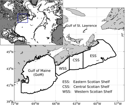
In this paper, historical simulations and projections from 22 CMIP6 ESMs for the Scotian Shelf and Gulf of Maine are analysed with a focus on sea surface temperature (SST) and ocean bottom temperature (BT). The reason for the choice of SST is that there are high-quality data sets available for historical validation. While there is substantially less BT data available, this is a critical ocean layer for many marine species that spend part of their life cycle near the seabed. An assessment of the CMIP6 ESM simulations is conducted using an SST product and in-situ bottom temperature datasets. To provide geographically detailed information on the hydrographic changes for the SS, the region is divided into three subareas: Eastern SS, Central SS, Western Scotian Shelf ().
Fig. 1 Map of research subareas. The outer edges of these areas are defined by the 200 m isobath. The inset at the top left shows the North Atlantic Ocean, and the location of the research region in this study (blue rectangle), and the solid lines indicate 200, 1000, 3000 m isobaths.
This paper is organised as follows. Section 2 will present the data and methods used in this study. Section 3 discusses the validation of models. Section 4 reports the projections for SST and BT from the 22 CMIP6 ESMs. Section 5 provides a discussion of the results.
2 Materials and methods
In this study, 22 CMIP6 ESMs and two climate scenarios were chosen () based on data availability and communication with the data providers as of 3 April 2021. The data were downloaded from the Earth System Grid Federation (ESGF; https://esgf-node.llnl.gov/search/cmip6), and details on these ESMs can be found there. lists the horizontal resolution of these 22 ESMs, showing that most of these models have horizontal resolution of ∼100 km, two of the 22 ESMs have resolutions of 25 km, and resolutions of the atmospheric component of the ESMs range from 100 to 500 km. The simulation cases analysed in this study are summarised in Supplementary Materials – Table S0.
Table 1. Summary of the 22 CMIP6 ESMs.
The HadISST1 dataset (https://www.metoffice.gov.uk/hadobs/hadisst/data/download.html; Rayner et al., Citation2003) was used to evaluate model solutions of SST. Bottom temperature (BT) is an ocean quantity with sparse observations in both temporal and spatial domains. However, DFO regular summertime surveys on the Scotian Shelf have broad spatial coverage and are the main source of historic BT data, and a gridded BT product (resolution: 0.2° by 0.2°) for the Scotian Shelf from 1970 onward has been created. This dataset has been successfully used in many studies, e.g. Brickman et al. (Citation2018). Brickman et al. (Citation2018) clearly demonstrated monthly mean (July) modelled BT from a North Atlantic model developed at Bedford Institute of Oceanography were consistent with the DFO summertime surveys. We use this dataset to assess BT performance of the ocean models in this study.
Data from 22 CMIP6 simulations for the period 1955–2049 are analysed, focusing on areal-average temperatures in the ESS, CSS, WSS and Gulf of Maine regions (). 1955–2014 is the period of historical simulation, 2015–2049 is the period of projected simulation.
For the historical period, model timeseries are compared to observations with model bias (Bs, defined in Supplementary Materials 1) and trend (Tr; unit: deg/decade) computed for each model. Ensemble trend and bias are calculated as the average trend and the average bias of the 22 CMIP6 ESMs, allowing for a standard deviation to be computed. (NB: the same approach is applied to similar ensemble calculations in the remainder of this study). A ranking system to assess model performance is included in the Supplementary Materials 3.
For the future climate period we selected two ssp scenarios: ssp245 and ssp370. (1) ssp245: Radiative forcing reaches a level of 4.5 Wm−2 in 2100. This scenario represents the medium part of the range of plausible future pathways. (2) ssp370: Radiative forcing reaches a level of 7.0 Wm−2 in 2100. This scenario represents the medium to high end of plausible future pathways. ssp370 fills a gap in the CMIP5 forcing pathways that is particularly important because it represents a forcing level common to several (unmitigated) ssp baselines. Projected trends (2020–2049) and changes (2030–2049 and 2040–2049 relative to 1995–2014) of the SST and BT for these regions were investigated.
3 Model performance
This investigation of ESM performance focuses on SST and BT using HadISST1 and BT from summertime surveys, respectively. Model bias and trend are the metrics used in assessing the model performance.
a Sea Surface Temperature
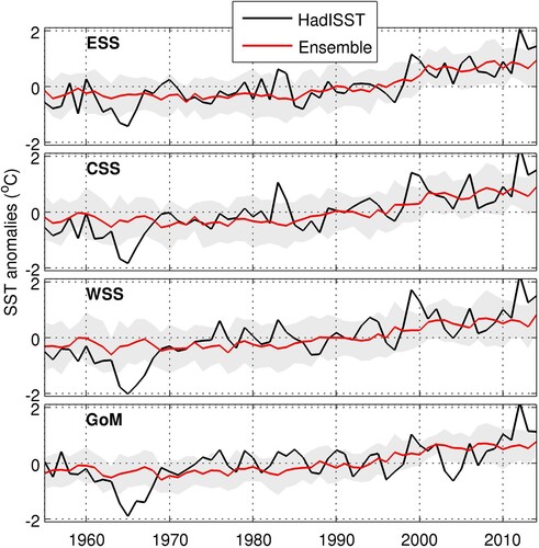
For SST, annual-mean time series for 1955–2014 from the 22 CMIP6 ESMs and the HadISST1dataset are used in the Bs and Tr calculations (). Most of the CMIP6 ESMs have warm biases for all the 4 subareas, although cold biases do exist in some ESMs. The number of ESMs with cold biases decreases from north (ESS) to south (GoM). Interestingly, all three high resolution ESMs (AWI-CM-1-1-MR, CNRM-CM6-1-HR, and MPI-ESM1-2-HR) show small cold biases for the 4 subareas. It is evident that there is a large range for the trends. All models show positive trends consistent with the HadISST1 data for all 4 subregions. Of the 88 model trend calculations (22 models × 4 regions), 11 have fractional errors <0.1. It is worth mentioning that the very cold period of the 1960s in the four regions were mostly missed by these above-mentioned models, and they are not represented in the ensemble means as well, which demonstrates issues with CMIP6 models in capturing extreme events occurring on decadal timescales.
Table 2. SST: The model bias (Bs; unit: deg) and trends (Tr; unit: deg/decade) for all time series, all calculated from time series of annual means, 1955-2014. Underlined: confidence level < 95%; Blue in brackets (in Tr title cell): trend in HadISST1.
With respect to model performance, CNRM-CM6-1, AWI-CM-1-1- MR and MPI-ESM1-2-HR demonstrate the best agreement with observations for the 4 subareas () and are the highest ranked models (Supplementary Materials 3, Table S15). Among these three models, AWI-CM-1-1-MR and MPI-ESM1-2-HR are high resolution ESMs.
To investigate the performance of the ensemble, the ensemble average bias and trend are shown in the last line of . The ensemble biases for the 4 subareas all have positive sign with the smallest bias of 0.78 °C for ESS, and the largest one of 2.72 °C for WSS. The ensemble trends from the 4 subareas are all smaller than the observed ones ().
Fig. 2 Time series of annual SST for ensemble mean from the 22 CMIP6 ESMs and HadISST1 data, 1955–2014. The shaded area denotes plus or minus one standard deviation of the 22 models. Units are degrees Celsius.
b Bottom Temperature
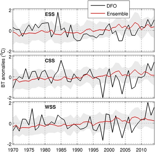
To assess ESM performance in simulating BT, we compare the July ESM time series to the July eco-system survey data for the ESS, CSS and WSS subareas, over the period 1970–2014. The in-situ BT data are only available for the Scotian Shelf subareas, so there is no analysis of bottom temperature for the Gulf of Maine in this paper. Drinkwater et al. (Citation2002) reported that there was little or no seasonal change at depths greater than approximately 100–150 m on the Scotian Shelf, hence it is not expected to see a large seasonal variability in BT there.
ESM performance varies and is neither consistent across measures (Bs, Tr) nor across subareas (). (Note that the trends for the observations are not significantly different from zero). Most of the CMIP6 ESMs have warm biases. The number of ESMs with cold BT bias for ESS is much smaller than for SST bias. Of note is that those ESMs with cold SST biases do not necessarily have cold BT biases, and the high-resolution ESMs do not have a reduced BT bias as they do for SST bias.
Table 3. July bottom temperature: Model bias (Bs; unit: deg) and trends (Tr; unit: deg/decade) for all time series, 1970-2014. Underlined: confidence level < 90%; Blue in brackets (in Tr title cell): trend values for DFO July survey data.
With respect to model performance, CNRM-ESM2-1 and NorESM2-LM demonstrate the best agreement with observations for the 3 subareas () and are the highest ranked models (Supplementary Materials 3, Table S16). Interestingly, the models with higher resolution (AWI-CM-1-1-MR, CNRM-CM6-1-HR, MPI-ESM1-2-HR) do not show consistent performance across subareas and are not among the highest ranked models, ranking 15, 12, 19 respectively (Supplementary Materials 3, Table S16).
With respect to simulating the trends in the observations, of the 66 model comparisons only 16 (24%) are consistent with the observed zero slope trend. Considering the nature of these air–sea–ice–land coupled models and complexity of factors for the BT variations, it is not surprising to see that almost all of the models fail to capture the observed trends of the BT.
With respect to ensemble mean calculations, and in contrast to the performance of the SST ensembles, the BT ensemble biases are all above 2 °C, with the largest one for ESS (3.54°C), and the smallest one for CSS (2.12°C) (). The BT ensemble trends are stronger than the observed ones, also in contrast to the SST ensemble results. July survey data (labelled ‘DFO’) and the ensemble mean from the 22 ESMs are shown in .
Fig. 3 Time series of the BT in July from the DFO ecosystem survey data and the ensemble from the 22 CMIP6 ESMs for the period of 1970-2014. The shaded area denotes plus or minus one standard deviation of the 22 models.
4 Projections of SST and BT
It is widely recognised in the climate science community that no single ESM is able to provide a robust representation of all of the important processes in the climate system, especially those affecting regional climate (Loder et al., Citation2015, and references therein). IPCC (The Intergovernmental Panel on Climate Change) projections are based on the statistics of an ensemble of models. Such an ensemble approach is also needed to represent regional climate. In this section, we focus on the ensemble mean projections of SST and BT.
a SST
1 SST trends
In this study, both annual means and seasonal means are investigated, and the definitions of the four seasons are winter (JFM), spring (AMJ), summer (JAS), and fall (OND). For all of the 22 CMIP6 ESMs (; Supplementary Materials: Tables S1–S5), most of the 4 regions’ 30-year trends have a range of ∼1°C/decade (maximum – minimum), with Gulf of Maine having the smallest range for annual means and seasons of winter and spring. Summer shows the smallest range for CSS/ssp245. The largest range occurs in WSS under ssp370. Some CMIP6 models project negative (cooling) trends; however, the number with negative annual trends is small (≤5), suggesting negative trends are unlikely. The ensemble means of the 30-year trends for historic (1985–2014) and projected (2020–2049; ssp245 and ssp370) periods are calculated for the annual means and seasonal periods ().
Fig. 4 Violin plots of SST and BT trends for all ESMs (ssp245: light red; ssp370: light blue). The boxes indicate the interquartile range (IQG), and whiskers are 1.5 IQR. The horizontal line is for mean value, and the white circle is for median value.
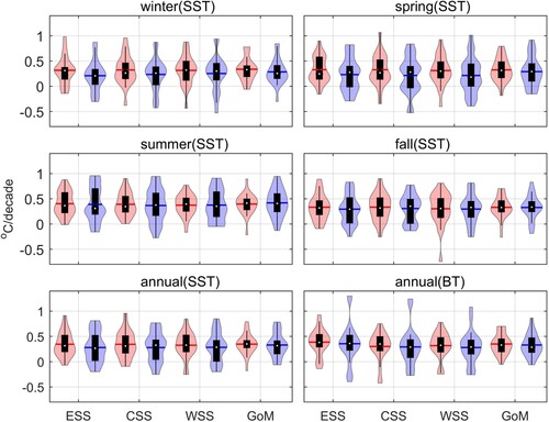
Table 4. Ensemble means of 30-year SST trends from CMIP6 ESMs under ssp245 and ssp370 for the 4 regions. Trends for historic period (1985–2014) are indicated by Hist. Unit: (°C/decade).
In all four regions the SST trends in summer are the largest among the four seasons both in the historical period and in the projected period.
In the annual means, the ESS has the strongest historical trend of 0.44 °C/decade and also the strongest projected trend of 0.35 °C/decade under ssp245. In the ESS and CSS, the projected trends under both scenarios are smaller than the historical ones, and the ssp245 trend is larger than the historical one in the WSS and GoM. We note that in general the ssp245 simulations have larger trends than the ssp370 ones (see Discussion).
In the seasonal means, ESS and CSS have projected trends smaller than the historical ones. WSS and Gulf of Maine have stronger projected winter and autumn trends compared to the historical trends.
2 SST changes
Projected SST changes are investigated by comparing historical (1995–2014) bi-decadal annual and seasonal means against two future periods, 2030–2049 (bi-decadal) and 2040–2049 (decadal). lists the ensemble means of the SST changes of decadal and bi-decadal periods under the two climatic scenarios. The changes for the seasonal and annual means are in the range of 1–1.8°C for all the four regions under both climate scenarios. Consistent with the trends in summer, the changes in summer are the strongest among the four seasons for both the bi-decadal and decadal periods for all the four regions. The decadal means are mostly 0.2 °C warmer than the bi-decadal ones, indicating that surface temperature continues to increase into the 2040–2049 period under these two climatic scenarios. Furthermore, other seasons are also ∼0.2 °C warmer in the decadal period. Details about projections from individual CMIP6 ESMs can be found in Supplementary Materials (Tables S6–S10). We note that the differences between the ssp245 and ssp370 scenarios for SST changes are very small (less than 0.1 °C).
Table 5. Projected bi-decadal (bd:2030–2049) and decadal (de: 2040–2049) ensemble mean changes of the SST relative to 1995–2014 period for the ssp245 (s2) and ssp370 (s3). Units are in °C.
b BT
In this subsection, we focus on the projected climate changes in annual mean BT using the same projected and historic periods as those used in the SST analysis.
1 BT trends
There is a widespread in the ranges of the 30-year trends with ssp370 having larger ranges than ssp245 (bottom right panel of ). The majority of CMIP6 ESMs project positive trends (warming; bottom-right panel of ), however, a small number of ESMs project a decrease in bottom temperatures (∼1/7, Supplementary Materials, Table S11). The averaged trends for all subareas, for both projections, are between 0.2 and 0.4°C/decade. Further details about the projected trends from each individual model can be found in the Supplementary Materials (Table S11). One interesting feature of the trends for the four regions under ssp370 is that the ranges of the trends gradually decrease from the eastern Scotian Shelf down to the Gulf of Maine.
lists the annual trends of the historical (1985–2014) and projected (2020–2049; ssp245 and ssp370) periods for all subareas. ESS has the largest trends of all subareas. ssp245 trends are greater than ssp370 trends for all subareas. The largest trend is ESS/ssp245 (0.39 °C/decade), the smallest is WSS/ssp370 (0.29 °C/decade). The projected trends for all of the four regions and under the two climatic scenarios are much larger than the historical ones, which is notably different from the result for SST.
Table 6. Ensemble mean trends of annual mean BT for each subarea, for the periods 1985–2014 (Hist) and 2020–2049 (ssp245 and ssp370). Units are °C/decade.
The models with better BT trend performance (i.e. CNRM-ESM2-1 and NorESM2-LM, in ) have trends similar to the ensemble, and trends from TaiESM1 are generally very close to the ensemble.
2 BT changes
lists the annual BT changes relative to the historical bi-decadal climatology for 1995–2014. All changes are positive (warming) with the ESS having the largest changes and the CSS having the smallest. For bi-decadal projections the difference between ssp245 and ssp370 is less than 0.1°C for all subareas except WSS. Details on the projected changes of each individual model can be found in Supplementary Materials (Table S12).
Table 7. Projected bi-decadal (bd:2030–2049) and decadal (de: 2040–2049) annual ensemble mean changes of BT relative to 1995–2014 period for ssp245 (s2) and ssp370 (s3). Units are in °C.
5 Discussion
This study investigated changes of SST and BT on the Scotian Shelf and in the Gulf of Maine using model solutions from 22 CMIP6 ESMs. Most of CMIP6 ESMs have coarse resolution for the ocean component (∼100 km horizontal), though some of the ESMs have resolutions of ∼25 km, which is considered to be an eddy-permitting resolution in the region of this study. For mid-latitudes of the North Atlantic Ocean, the barotropic Rossby radius is of order 100 km; however, the first baroclinic Rossby radius ranges from 10–30 km (Chelton et al., Citation1998). This suggests that these ESMs can represent barotropic processes at smaller scales, but not baroclinic ones. The extent to which coarse resolution CMIP6 ESMs can represent shallow continental shelf waters like the Scotian Shelf and Gulf of Maine remains an open question for two main reasons. First, because the interaction between poleward transport of the Gulf Stream and equatorward transport of the Labrador Current requires high resolution ocean models to properly resolve the dominant physical processes; and second because part of the onshelf variability in this region is due to inflows through narrow channels which are not resolved by coarse resolution models (Brickman et al., Citation2018).
We analysed the model SST simulations (see Supplementary Materials 4) to see whether a similar hot model problem exists for our region. We find that the hottest models in the present climate (historical period) are also the hottest models in 2050. Considering the regional average SST changes in 2050 (relative to present climate data), we find that the majority of models (14) have changes between 1.6 and 4.6 °C, but there are five “hot models” with changes ≥ 5.4 °C (three ≥6.9 °C). If we eliminate the five hottest models from the ensemble average projections, we get reductions in SST changes for the four regions (ESS, CSS, WSS, GoM) from 2.3, 3.2, 4.2, 3.9 °C down to 1.6, 2.1, 3.1, 3.0 °C respectively. While our analysis is much simpler than that of the IPCC authors, it does suggest that ensemble average SST projections in particular regions may also exhibit hot model bias.
The positive trends in the HadISST1 in the four regions are observed in all 22 models, and some of the models have trends close to that of the HadISST1 data. The insignificant observed BT trends for the three subareas of the Scotian Shelf are mostly missed by the 22 models, and those high-resolution models do not present better skills in obtaining observed trends than coarse resolution models. In general, for BT, the ESMs with higher resolutions do not perform better than the coarse-resolution ones (Table S17, columns 7–9). Saba et al. (Citation2016) demonstrated that a high-resolution model is needed for the simulation and projection of the BT of the Scotian Shelf and Gulf of Maine, while our investigation of these CMIP6 ESMs does not show that increasing resolution enhances the model performance in terms of representing observed trends (although we note that the resolution of these ESMs is still coarser than Saba’s CM2.6 model). The high-resolution models (AWI-CM-1-1-MR, CNRM-CM6-1-HR, and MPI-ESM1-2-HR) do show smaller SST biases for the four regions, but this is not apparent in the BT biases.
We need to mention that the model biases of SST and BT relative to the data used in this study could change if a different set of data is used, but the changes in the biases should only be a shift in the biases, not the differences among them.
Providing better climate projections is an important goal of the climate research community. An ensemble approach is a commonly adopted method, and other approaches derived from this method have also been applied, such as the model-performance based ensemble approach suggested by Overland et al. (Citation2011). In our analysis, we have noted that some models demonstrate better performance at simulating historical trends among the 22 ESMs but have projected trends quite different from the ensemble mean (e.g. CESM2, see and Table S1 for ESS/ssp245). However, there are models that perform well in simulating past trends but also have projections that align well with the ensemble estimates (e.g. CNRM-CM6-1-HR, see and Table S1). Further investigation into various ensemble approaches for improving projections should remain as a research priority.
It should be noted that an ESM with a trend close to the ensemble SST projection may not necessarily produce a trend close to the ensemble BT projection. Also noteworthy is that good model performance on representing two metrics of the historic SST does not necessarily lead to good performance on BT. This raises a question about how to project quantities without historic observations to examine ESM performance, if model-performance based ensemble methods are the approach used for climate projection.
Brickman et al. (Citation2021) investigated the SST changes in the Gulf of Maine using two high-resolution regional ocean models representing four simulations under the RCP8.5 scenario, and reported an SST increase of 1.1 –2.4 °C and a BT increase of 1.5–2.1 °C in 2050 relative to 1976–2005. Using the ensemble mean of the 22 CMIP6 ESMs for ssp245 and ssp370, our study reports an SST increase between 1.5 °C to 1.6 °C and a BT increase of 1.4 °C for the 2040–2049 period relative to 1995–2014. While the scenarios from these two studies, and the historical reference periods used, are different, the magnitudes of the trends are similar.
We noticed the projected SST trends for ESS and CSS are smaller than historical ones, while WSS and Gulf of Maine have stronger winter and autumn trends than historical ones. We suspect that increasing cold waters from glacier and Arctic ice melting are most likely the cause for this phenomenon. ESS and CSS are the regions that could be more vulnerable to the increasing cold waters than WSS and Gulf of Maine in general due to their geographic location, while the WSS and Gulf of Maine can experience more impacts from the Gulf Stream due to their location as well, and it is generally known that the Gulf Stream is projected to move northward, allowing warm Gulf Stream water into these two regions, and this impact is more obvious in winter and autumn. Further studies are needed to better understand this interesting phenomenon.
One interesting phenomenon is that the ranges of projected BT trends under the two climatic scenarios (bottom right panel of ), exhibit a pattern of gradual decrease from the eastern Scotian Shelf to the Gulf of Maine, particularly for ssp370. Peterson et al. (Citation2017) reported that subsurface temperature in the region off the Scotian Shelf was linked to wind stress curl pattern in the mid-Atlantic, suggesting the importance of wind in the subsurface temperature. Air temperature increases induced by increasing greenhouse gas emissions are generally well understood, but how well the air temperature increases can be translated into changes in the atmospheric circulation (wind) in the ESMs is very uncertain (Shepherd, Citation2014). Parameterizations, numerical approaches, model horizontal and vertical resolutions, and other factors, can all lead to different representations of the atmospheric circulation by these models, which is beyond the scope of our current study to analyse. Future study is needed to understand forcing mechanisms driving BT variations in this region.
Another interesting phenomenon is that the ensemble trends and relative changes in SST of the ssp245 are generally higher than those of ssp370 (). Higher greenhouse gas emissions in ssp370 should lead to higher ocean surface temperature, however the projections from the ESMs do not support this. The temperature uncertainties represented by the standard deviations for ssp370 are mostly larger than those for the ssp245 (). We speculate that the increased greenhouse gas emissions in ssp370 probably lead to greater inter-model variability in the wind fields and more variable ocean circulation, resulting in lower projected trends and relative changes. Another possibility is that further increases in Arctic ice melt and introduction of fresh and cold water could lead to this phenomenon as well. Ultimately, the reason for a weaker response in ssp370 requires further study.
Supplemental Material
Download MS Word (150.1 KB)Acknowledgements
Drs. Ryan Stanley and Simon Higginson provided helpful comments for an early version of the MS. Discussions with Dr. John Loder helped Z.W. better understand the climate system, and its changes.
Disclosure statement
No potential conflict of interest was reported by the author(s).
Supplemental data
Supplemental data for this article can be accessed online at https://doi.org/10.1080/07055900.2023.2264832.
Additional information
Funding
References
- Brickman, D., Alexander, M. A., Pershing, A., Scott, J. D., & Wang, Z. (2021). Projections of physical conditions in the Gulf of Maine in 2050. Elementa: Science of the Anthropocene, 9(1), 00055. https://doi.org/10.1525/elementa.2020.20.00055
- Brickman, D., Hebert, D., & Wang, Z. (2018). Mechanism for the recent ocean warming events on the Scotian Shelf of eastern Canada. Continental Shelf Research, 156, 11–22. https://doi.org/10.1016/j.csr.2018.01.001
- Chelton, D. B., deSzoeke, R. A., Schlax, M. G., El Naggar, K., & Siwertz, N. (1998). Geographical variability of the first baroclinic Rossby radius of deformation. Journal of Physical Oceanography, 28(3), 433–460. https://doi.org/10.1175/1520-0485(1998)028<0433:GVOTFB>2.0.CO;2
- Drinkwater, K. F., Petrie, B., & Smith, P. C. (2002). Hydrographic variability on the Scotian Shelf during the 1990s. Northwest Atlantic Fisheries Organization (NAFO). Scientific Council Meeting – June 2002. Serial No. N4653. SCR Doc.02/42.
- Gonçalves Neto, A., Palter, J. B., Xu, X., & Fratantoni, P. (2023). Temporal variability of the Labrador current pathways around the tail of the grand banks at intermediate depths in a high-resolution ocean circulation model. Journal of Geophysical Research: Oceans, 128(3), e2022JC018756. https://doi.org/10.1029/2022JC018756
- Greenan, B., Shackell, N., Ferguson, K., Greyson, P., Cogswell, A., Brickman, D., Wang, Z., Cook, A., Brennan, C., & Saba, V. (2019). Climate change vulnerability of American lobster fishing communities in Atlantic Canada. Frontiers in Marine Science, https://doi.org/10.3389/fmars.2019.00579
- Han, G., Loder, J. W., & Smith, P. C. (1999). Seasonal-mean hydrography and circulation in the Gulf of St. Lawrence and on the eastern Scotian and southern Newfoundland shelves. Journal of Physical Oceanography, 29(6), 1279–1301. https://doi.org/10.1175/1520-0485(1999)029<1279:SMHACI>2.0.CO;2
- Hannah, C. G., Shore, J. A., Loder, J. W., & Naimie, C. E. (2001). Seasonal circulation on the western and central Scotian Shelf. Journal of Physical Oceanography, 31(2), 591–615. https://doi.org/10.1175/1520-0485(2001)031<0591:SCOTWA>2.0.CO;2
- Hausfather, Z., Marvel, K., Schmidt, G. A., Nielsen-Gammon, J. W., & Zelinka, M. (2022). Climate simulations: recognize the ‘hot model’ problem. Nature, 605(7908), 26–29. https://doi.org/10.1038/d41586-022-01192-2
- Hebert, D., & Pettipas, R. G. (2016). Physical Oceanographic Conditions on the Scotian Shelf and in the eastern Gulf of Maine (NAFO Division 4 V,W,X) during 2015. Northwest Atlantic Fisheries Organization (NAFO), Scientific Council Meeting – June 2016. Serial No. 6542. SCR Doc.16/06.
- Loder, J. W., Baaren, A., & Yashayaev, I. (2015). Climate comparisons and change projections for the northwest Atlantic from Six CMIP5 models. Atmosphere-Ocean, 53(5), 529–555. https://doi.org/10.1080/07055900.2015.1087836
- Loder, J. W., Han, G., Hannah, C. G., Greenberg, D. A., & Smith, P. C. (1997). Hydrography and baroclinic circulation in the Scotian Shelf region: Winter versus summer. Canadian Journal of Fisheries and Aquatic Sciences, 54(S1), 40–56. https://doi.org/10.1139/f96-153
- Loder, J. W., Petrie, B., & Gawarkiewicz, G. (1998). The coastal ocean off north-eastern North America: A large-scale view. In A. R. Robinson, & K. H. Brink (Eds.), The Sea 11 (pp. 105–133). Wiley.
- Meehl, G. A., Covey, C., Taylor, K. E., Delworth, T., Stouffer, R. J., Latif, M., McAvaney, B., & Mitchell, J. F. B. (2007). The WCRP CMIP3 multimodel dataset: A new era in climate change research. Bulletin of the American Meteorological Society, 88(9), 1383–1394. https://doi.org/10.1175/BAMS-88-9-1383
- Overland, J. E., Wang, M., Bond, N. A., Walsh, J. E., Kattsov, V. M., & Chapman, W. L. (2011). Considerations in the selection of global climate models for regional climate projections: The Arctic as a case study. Journal of Climate, 24(6), 1583–1597. https://doi.org/10.1175/2010JCLI3462.1
- Peterson, I., Greenan, B., Gilbert, D., & Hebert, D. (2017). Variability and wind forcing of ocean temperature and thermal fronts in the Slope Water region of the Northwest Atlantic. Journal of Geophysical Research: Oceans, 122(9), 7325–7343. https://doi.org/10.1002/2017JC012788
- Petrie, B. (2007). Does the North Atlantic Oscillation affect hydrographic properties on the Canadian Atlantic continental shelf? Atmosphere-Ocean, 45(3), 141–151. https://doi.org/10.3137/ao.450302
- Rayner, N. A., Parker, D. E., Horton, E. B., Folland, C. K., Alexander, L. V., Rowell, D. P., Kent, E. C., & Kaplan, A. (2003). Global analyses of sea surface temperature, sea ice, and night marine air temperature since the late nineteenth century. Journal of Geophysical Research, 108(D14), 4407. https://doi.org/10.1029/2002JD002670
- Saba, V. S., Griffies, S. M., Anderson, W. G., Winton, M., Alexander, M. A., Delworth, T. L., Hare, J. A., Matthew J. Harrison, Rosati, A., Vecchi, G. A., & Zhang R. (2016), Enhanced warming of the Northwest Atlantic Ocean under climate change, J. Geophys. Res. Oceans, 121, 118– 132, doi:10.1002/2015JC011346.
- Shepherd, T. (2014). Atmospheric circulation as a source of uncertainty in climate change projections. Nature Geoscience, 7(10), 703–708. https://doi.org/10.1038/ngeo2253
- Stanley, R., DiBacco, C., Lowen, B., Beiko, R., Jeffery, N., Wyngaarden, M., Bentzen, P., Brickman, D., Benestan, L., Ber Natchez, L., Johnson, C., Snelgrove, P., Wang, Z., Wringe, B., & Bradbury, I. (2018). A climate-associated multispecies cryptic cline in the northwest Atlantic. Science Advances, 4(3), https://doi.org/10.1126/sciadv.aaq0929
- Taylor, K. E., Stouffer, R. J., & Meehl, G. A. (2012). An overview of CMIP5 and the experiment design. Bulletin of the American Meteorological Society, 93(4), 485–498. https://doi.org/10.1175/BAMS-D-11-00094.1
- Townsend, D. W., Thomas, A. C., Mayer, L. M., Thomas, M. A., & Quinlan, J. A. (2006). Oceanography of the northwest Atlantic continental shelf (1, W). In A. R. Robinson, & K. H. Brink (Eds.), The sea (pp. 119–168). Harvard University Press.
- Wang, Z., Horwitz, R., Bowlby, H., Ding, F., & Joyce, W. (2020). Changes in ocean conditions and hurricanes affect porbeagle Lamna nasus diving behavior. Marine Ecology Progress Series, 654, 219–224. https://doi.org/10.3354/meps13503
- Wang, Z., Lu, Y., Dupont, F., Loder, J., Hannah, C., & Wright, D. (2015). Variability of sea surface height and circulation in the North Atlantic: Forcing mechanisms and linkages. Progress in Oceanography, 132, 273–286. https://doi.org/10.1016/j.pocean.2013.11.004
- Wang, Z., Yang, J., Johnson, C., & DeTracey, B. (2022). Changes in deep ocean contribute to a “See-sawing” gulf stream path. Geophysical Research Letters, 49, e2022G–L100937. https://doi.org/10.1029/2022GL100937
- Weare, B. C. (1977). Empirical orthogonal analysis of Atlantic Ocean surface temperatures. Quarterly Journal of the Royal Meteorological Society, 103(437), 467–478. https://doi.org/10.1002/qj.49710343707
- Yang, J., & Chen, K. (2021). The role of wind stress in driving the along-shelf flow in the northwest Atlantic Ocean. Journal of Geophysical Research: Oceans, 126(4), e2020JC016757. https://doi.org/10.1029/2020JC016757