A Circulation Model for Baynes Sound, British Columbia, Canada

ABSTRACT

An application of the three-dimensional Finite Volume Community Ocean Model was developed for Baynes Sound, British Columbia, Canada and a simulation was carried for the period of May 2016 to April 2017. The objective was to provide highly resolved spatial estimates of the regional hydrodynamics that could be used in a coupled biogeochemical model to assess the cultured shellfish carrying capacity of the region. The issue of how representative the particular simulation period was in the context of typical seasonal features was addressed by comparing temperatures, salinities and river discharges with long-term statistics. Circulation model results were generally in good agreement with salinity, temperature, velocity, and sea surface height observations, providing confidence in subsequent seasonal estimates of volume fluxes through the two entrances and water-renewal. Approximately sixty percent of the variability in near-surface temperature observations at five locations was shown to be linearly dependent on a combination of the along-sound wind, air temperature, and the daily sea surface range, which was taken as a proxy for tidal mixing.

RÉSUMÉ

[Traduit par la rédaction] Une application du modèle tridimensionnel «Finite Volume Community Ocean Model» a été développée pour Baynes Sound, en Colombie-Britannique, au Canada, et une simulation a été réalisée pour la période allant de mai 2016 à avril 2017. L’objectif était de fournir des estimations spatiales à haute résolution de l’hydrodynamique régionale qui pourraient être utilisées dans le couplage d’un modèle biogéochimique pour évaluer la capacité de charge de la région pour les mollusques et crustacés d’élevage. La question de la représentativité de la période de simulation considérée dans le contexte des caractéristiques saisonnières typiques a été abordée en comparant les températures, les salinités et les débits fluviaux avec les statistiques à long terme. Les résultats du modèle de circulation concordaient généralement bien avec les observations en matière de salinité, de température, de vitesse et de hauteur du niveau de la mer, ce qui a permis d’avoir confiance dans les estimations saisonnières ultérieures des flux de volume à travers les deux entrées et le renouvellement de l’eau. Environ 60% de la variabilité des observations de la température proche de la surface à cinq endroits s’est avérée dépendre linéairement d’une combinaison de la composante longitudinale du vent, de la température de l’air et de l’amplitude quotidienne de la surface de la mer, considérée comme une approximation du mélange maréal.

KEYWORDS:

• Baynes Sound
• FVCOM
• circulation model
• water renewal

1 Introduction and motivation

Baynes Sound, a narrow channel off east central Vancouver Island, is approximately 30 km long, 0.6 to 3.8 km wide at low tide, and bounded on the east by Denman Island (Fig. 1). Although there are northern and southern openings to the Strait of Georgia (SOG), the northern channel (Comox Bar) narrows considerably at lowest normal tides and has only a maximum depth of 4 m. The width of the southern entrance narrows with a falling tide, where the distance across the surface water ranges between 1.6 km at high tide and 0.6 km at low tide. With a maximum water depth of 42 m, the southern entrance serves as the primary conduit for water exchange with the SOG. Depths shallow from about 60 to 40 m along a trough in the central sound and attain a maximum depth of 90 m in a hole near the southern entrance. There are extensive tidal flats along the Vancouver Island coast, at the mouth of the Courtenay River delta and extending northward off Denman Island. Flood tides enter from the SOG at both entrances but due to the greater volume transports in the south, tidal phases progress northward along the central sound (Canadian Hydrographic Service chart 3527). However, the fact that no speeds are shown on this chart indicates a lack of observations.

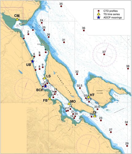
Fig. 1 Regional map of Baynes Sound showing CTD stations and locations of ADCP moorings (UB: Union Bay; BCF: BC Ferries) and temperature-salinity time series observations (CM: Comox Marina; LS: Lucky Seven; FB: Fanny Bay; MO: Mac’s Oysters; CI: Chrome Island; HT: Hornby Terminal). The base map showing bathymetric contours (blue) and mudflat regions (green) was modified from the Canadian Hydrographic Service nautical chart #3527. CTD Stations 39 and 40 are outside of map coverage and are located east of Hornby Island roughly extending the line of Stations 35 to 38.

Baynes Sound has a high diversity of shellfish habitats made up of intertidal mud and sand flats, rocky shorelines, and an extensive sandbar at the Northern entrance bordering the subtidal basin and channel. Shellfish aquaculture in British Columbia dates back to the 1920s, with Baynes Sound becoming the dominant shellfish producer over time (Barnes, 2007; BC Ministry of Sustainable Resource Management, 2002; Richardson & Newell, 2002). Although both wild and farmed clams have been harvested since the 1940s, the total shellfish production has recently become dominated by Pacific oyster production (Carswell et al., 2006). In 2019, the weight and dollar value for oysters (7,783 tonnes; $15,246,000), clams (1,114 tonnes; $6,972,000), mussels (727 tonnes; $4,135,000) and scallops (76 tonnes; $629,000) contributed to 52%, 59%, 3%, and 93% of the total Canadian shellfish landings, respectively (DFO, 2022). In the past, coastal management plans and spatial analysis have been undertaken to assess the status of shellfish production in Baynes Sound (BCM-SRM, 2002; Carswell et al., 2006).

Using results from extensive field studies carried out in 2002, Hay and Company Consultants (2003, henceforth HCC03) developed and validated ocean circulation and biogeochemical models to assess the carrying capacity of the region. Although HCC03’s conclusion was that “the commercial bivalve population is functioning at a level well below the maximum bivalve carrying capacity of Baynes Sound”, local oyster and clam production tonnages have respectively increased by factors of 2.6 and 1.5 from 2001 (HCC03) to 2015. Given the increase shellfish production and changes to shellfish tenures, it is timely to update the carrying capacity assessment with a spatially-explicit, high-resolution hydrodynamic model, the Finite Volume Community Ocean Model (FVCOM) (Foreman et al., 2015). The project motivation was to develop a coupled FVCOM-BiCEM model (Bivalve Culture Ecosystem Model) that is accessible to a broad spectrum of people, including regulatory sectors managing shellfish resources, including scientists, shellfish industry, local interest groups, and urban planners. Previous efforts had been carried out only through local, private sectors.

The objective of this study is to assist the Department of Fisheries and Oceans (DFO) in managing the shellfish industry in Baynes Sound by improving on the HCC03 circulation model by, for example, 1) refining its spatial resolution at a bivalve-farm scale; 2) allowing the wetting-and-drying of mudflats that influences clam feeding frequency estimates; 3) including better atmospheric forcing reflecting a more accurate representation of regional hydrodynamics; and 4) increasing resolution of water renewal time estimates by including both the surface and bottom layers. In turn, these increased model sensitivities enhanced the coupled biogeochemical model and provided confidence in the recent estimates of nutrient-seston-bivalve interactions across a regional carrying capacity assessment (Guyondet et al., 2022).

Although other circulation models have been developed for the Salish Sea, FVCOM was validated for Baynes Sound, a smaller adjoining inlet, where a bay-wide, highly refined spatial resolution was required to assess shellfish farm-to-farm interactions (Fig. 1). In particular, FVCOM includes a 40-m horizontal grid that provides much higher spatial-resolution within Baynes Sound relative to four previous circulation models that included the Salish Sea: 1) a Regional Ocean Modeling System (ROMS: Masson & Fine, 2012) application with 3 km resolution for the entire BC coast; 2) the same grid and ROMS dynamics expanded to include a geochemical model assessing potential nutrient limitation, oxygen depletion, and plankton productivity (Peña et al., 2016); 3) an application of the Nucleus for European Modelling of the Ocean (NEMO 3.6; Soontiens & Allen, 2017) with 500-m grid resolution to assess mixing and advection of a sill-basin estuarine system; and 4) a biogeochemical model (Khangaonkar et al., 2012), wherein Baynes Sound was represented by a single grid element without bordering islands. In general, these Salish Sea models are more suitable for large coastal systems exposed to broad-scale bathymetry, current regimes, and atmospheric settings in Strait of Georgia, while FVCOM provided sensitivity at the shellfish farm scale to allow the coupled FVCOM-BiCEM to detect interactions between phytoplankton and shellfish production (Guyondet et al., 2022).

Accomplishments toward the project objective will be described in this manuscript and they will contribute to future aquaculture carrying capacity assessments accounting for potential impacts associated with ever-evolving bivalve culture techniques, adaptive governance compliance standards, and climate change promoting ocean acidification (Filgueira et al., 2016; Guyondet et al., 2014; Haigh et al., 2015; Steeves et al., 2018).

HCC03 provided a solid foundation for this present study. Its physical oceanographic field component took place from May 13, 2002 to November 21, 2002 with a period of intense data collection from September 17 to September 20. Two types of data were collected. The first were profiles of temperature (T), salinity (S), density, turbidity, and fluorometry obtained at a standard set of stations using a CTD (conductivity-temperature-depth) probe, while the second consisted of water velocity observations along thirty-four cross-sound transects using a ship-mounted ADCP (Acoustic Doppler Current Profiler). Appendix B in HCC03's Carrying Capacity Report shows thirteen three-dimensional plots of temperature and salinity along the thalwegs of Baynes Sound and Lambert Channel between May 13 and September 19 of 2002, while Appendix D shows similar plots of phytoplankton and zooplankton density. Comparisons between these data and our more recent TS profiles are described later in this study. Appendix C in HCC03's Carrying Capacity Report shows thirty-four snapshots of the east–west and north–south model velocities along transects crossing Baynes Sound over the period of September 17–19, 2002 and they are compared with similar plots in Appendix C of the Field Data Report (HCC03, 2003).

The modelling component of the HCC03 study encompassed three telescoping grids. The first covered the Salish Sea with 2-km horizontal resolution, the second covered Baynes Sound and Lambert Channel with 200-m resolution, while the third had 15-m resolution and focused on tide-induced upwelling in the region around Shingle Point in Lambert Channel. The models were run sequentially with boundary forcing for the second taken from the first and boundary forcing for the third taken from the second. The finite difference numerical approximations in each model were Hay and Company’s update of those described in Stronach et al. (1993) and Crean et al. (1988). Temperatures and salinities from the Baynes Sound circulation model were evaluated through comparisons with CTD data collected in May, June, August, and September, while velocities were compared against ADCP observations taken in September 2002. Both the modelled and measured salinity values were found to be in relatively good agreement in all cases except June, where discrepancies were attributed to inaccuracies in initializing the Salish Sea model and prescribing Fraser River discharges into it. Agreement between modelled and observed velocities was found to be highly dependent on the stage of the tide, where the best agreement was observed during strong flood and ebb tidal periods, and the poorest agreement was observed when the currents were weak. However, since the primary purpose of the circulation model was to study the transport of nutrients and water replenishment for bivalve feeding, current accuracy is most important during flood and ebb. HCC03, therefore, concluded that this good agreement was sufficient to deem the model simulations as acceptable. In addition to coupling with a biogeochemical model, the circulation model was also used to determine the residence time of water within Baynes Sound by following the fate of a tracer, over a 30-day period, that was initially distributed uniformly in the Sound. They found that the e-folding time, i.e. the time for the amount of tracer to reduce to 37% of its initial value, was 15.8 days.

The remainder of this paper is organized as follows. In section 2, the new circulation model and observational data are described, and 2016–17 temperatures, salinities, and river discharges are compared with long term averages in order to determine their representativeness in the context of other years. In section 3, the model results are evaluated with available observations while section 4 analyses the oscillations in five temperature time series. Section 5 estimates the seasonal volume fluxes through the northern and southern entrances to Baynes Sound, while section 6 estimates water renewal times throughout the sound. Finally, section 7 presents a brief summary, and discusses future work, including coupling between FVCOM and a biogeochemical model.

2 The circulation model and observational data

a Circulation model

The circulation model employed in this study is the Finite Volume Community Ocean Model (FVCOM) developed by Chen et al. (2003, 2006a, 2006b, 2011). FVCOM solves the 3D hydrodynamic equations for velocity and surface elevation and 3D transport/diffusion equations for salinity and temperature in the presence of turbulent mixing. It can be forced with any combination of tides, wind, river runoff, surface heating, and open ocean inflows and can also be coupled to biogeochemical and sediment transport components. The particular code employed (version 4.1) is a more recent version of that used in previous applications to the British Columbia coast (Foreman et al., 2009; Foreman et al., 2012). Further details on FVCOM and a more complete list of publications that have used it can be found at http://fvcom.smast.umassd.edu/FVCOM/index.html.

FVCOM has a sizeable user community in Canada, having been applied not only to general ocean and lake circulation problems, but also to specifically help understand dispersion around salmon farms in B.C., New Brunswick (Page et al., 2014), and Newfoundland (Ratsimandresy et al., 2020). It was for this reason, and the flexibility its triangular grid allows in better fitting the coastline, that FVCOM was chosen to simulate the hydrodynamics of Baynes Sound. However, unlike the previous B.C. applications to generally steep-sided fjords and inlets, a wetting-and-drying capability was included to more accurately capture the effects of extensive mudflats in the region. The accuracy of this feature has been confirmed in the New Brunswick applications where the large Bay of Fundy tidal range plays an important role in local hydrodynamics.

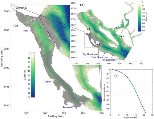
In the horizontal, the Baynes grid is comprised of irregularly sized triangles covering the northern half of the SOG (side lengths vary from approximately 4 km in the central strait to 40 m in Baynes Sound (Fig. 2a and b)), while in the vertical there are 20 unequally-spaced layers (Fig. 2c). As seen in Fig. 2c, the layer thickness when expressed as a fraction of the total depth has been chosen to be much smaller near the surface in order to better resolve the freshwater lens and the transmission of wind energy and heat flux to the upper ocean. The relative thickness then increases down the water column so that the bottom layer covers approximately 8% of the total depth. As subsequent temperature and salinity plots show there is little variation in the lower portions of the water column, this coarser resolution is sufficient.

Fig. 2 Triangular grid and bathymetry for the circulation model. (a) for the entire model domain showing the mouths of the Englishman, and Little and Big Qualicum rivers, (b) close-up view of Baynes Sound area with the Courtenay, Trent, Tsable, and Rosewall Rivers included in the model, and (c) bounds of the model vertical layers. Panel (a) includes tide gauge locations later used to evaluate the model: (1) Comox; (2) Little River; (3) Hornby Island; (4) Irvines Landing; and (5) Saltery Bay. Dashed lines in Panel (b) show transect lines across which volume fluxes are later calculated.

The model bathymetry was generated from Canadian Hydrographic Service (CHS) single-beam acoustic surveys with multi-beam soundings included where available. However, in order to reduce the ‘hydrostatic inconsistency’ and spurious currents (Haney, 1991) that can result with terrain-following vertical layers and steep bathymetry, as is found in some regions here, all depths were smoothed with a volume preserving technique that limits the ratio Δh/h within each triangle, where Δh is the difference between maximum and minimum depth and h is the average depth. This smoothing follows Hannah and Wright (1995) and is similar to the criteria recommended by Mellor et al. (1994).

The model is forced with i) the five tidal constituents M₂, S₂, N₂, K₁, and O₁ comprising approximately 76% of the total tidal height range at Comox; ii) climatological dynamic ocean topography (DOT) for summer and winter seasons; iii) freshwater discharge from four rivers emptying into Baynes Sound; and iv) winds and heat flux from the Environment and Climate Change Canada (ECCC) High Resolution Deterministic Prediction System (HRDPS) atmospheric model covering western Canada with 2.5 km horizontal resolution at two points across Baynes Sound. The M2 and K1 elevation amplitudes and phases were interpolated from Foreman et al. (2004). The remaining constituent harmonics were estimated using amplitude ratios and phase differences relative to the M2 (semi-diurnals) or K1 (diurnals) values at Comox. Though including the next three largest tidal constituents would increase the percentage of tidal height range explained to 87%, it is unlikely that this additional tidal energy would make much difference to subsequent results with a biogeochemical model. As will be seen, tidal current power measured at the two acoustic Doppler current profiler (ADCP) deployments in central Baynes Sound accounted for only a relatively small percentage of the total. Most of the power was in the sub-tidal frequency bands and attributable to variations in a combination of winds, river discharges, and inputs from the SOG. The only non-tidal component of sea surface height at the lateral boundaries was obtained from the average summer and winter DOT values from Foreman et al. (2008). We assumed the winter and summer values were for the season mid-points (Feb 15 and Aug 15) and then fit a sinusoid to obtain the values for each time step. Daily freshwater runoff for Courtenay, Trent, Tsable, and Rosewall rivers were included in the model. The mean annual freshwater discharge flow values included in the model are as follows: Courtenay River (51.3 m³s⁻¹), Trent (4.3 m³s⁻¹), Tsable (7.8 m³s⁻¹), and Rosewall Rivers (2.6 m³s⁻¹) (Braybrook et al., 1995; Riddell & Bryden, 1996)

Three-dimensional temperature and salinity fields interpolated from observations (conductivity, temperature, depth (CTD)) in the region were used to initialize the model and to specify temperatures and salinities along the northern and southern model boundaries during the model simulations. These fields were obtained as a sum of monthly climatological values and monthly anomalies. The climatological values were gridded from all available measurements within each calendar month between 1976 and 2016 and the anomaly fields were gridded from the differences between observations for the specific month and year and climatologies. The resulting fields are sufficiently realistic and smooth to serve as the model initial conditions without the need for lengthy spin-up. The model was spun-up during the first five days of simulation (April 25 to May 1, 2016), when the tides and other forcing were gradually brought to their full range. The spin-up time was excluded from all subsequent analyses.

FVCOM is linked to the Generalized Ocean Turbulence Model (GOTM; Burchard et al., 1999; Umlauf & Burchard, 2003), which offers several vertical mixing scheme choices. The results presented here were obtained with the Mellor-Yamada 2.5 scheme (MY2.5; Mellor & Yamada, 1982) and the same vertical mixing coefficient in both the velocity and temperature/salinity equations. Though FVCOM applications in other B.C. regions typically employed k-ϵ turbulent mixing, comparisons with results from MY2.5 in the Discovery Islands (Foreman et al., 2012) demonstrated that the particular choice made little difference to vertical profiles of velocity. Horizontal diffusion is parameterized with a Smagorinsky (1963) method whose formulation is described in Chen et al. (2008). Several coefficient values were tested before compromising on the value 0.02 m²s⁻¹ in the salinity and temperature transport/diffusion equations and 0.2 m²s⁻¹ for the momentum equations. These values provided reasonably smooth velocity fields and attempted to minimize potential contribution that horizontal mixing can make to vertical mixing in regions with steep bathymetry. In FVCOM, horizontal diffusion “occurs only parallel to” the vertical layers and this simplification can lead to overly diffusive model thermoclines and haloclines when those layers have significant slopes (Chen et al., 2006b).

b 2016–2017 temperature, salinity, and river discharge in the context of other years

Physical water-column variables, required to support both FVCOM and a coupled bivalve-aquaculture carrying capacity model, were collected with varying frequency and spatial resolution in Baynes Sound depending on modelling requirements and resources available. Vertical profiles of temperature, salinity, and oxygen were collected using a profiling Seabird-911 CTD (conductivity, temperature, depth) equipped with a 24 Niskin-bottle Rosette. For the most part, CTD profile surveys were carried out in the spring and summer periods between 2009 and 2019 in Baynes Sound and the Northern SOG (boundary zone) as part of the Ecosystem Research Initiative (ERI), the Program for Aquaculture Regulatory Research (PARR), and an Aquaculture Management Division (AMD) request for advice.

In general, central-axis stations (2, 5, 8, 11, 14, 17, 20, 22, and 23) were surveyed annually with the exception of 2010, 2015, and June 2017 (3-station tidal series) (Table S1). The number of sampling stations increased during this sampling period from 23 (inside BS) to 40 in order to increase spatial coverage in the boundary zone for the modelling period (2016–2017). Hourly tidal-series of vertical CTD profiles (Seabird-911-Rosette) at 3 fixed stations (ST2-upper, ST17-lower, ST23-outer Baynes Sound) were collected in both April and June of 2017. Additional CTD data were available from local DFO monitoring programs that provided increased spatial and temporal coverage within the entire modelling domain. Stations 39 and 40 are located in line with stations 35 to 38 with an equal inter-station distance.

In addition to CTD vertical profiles, portable YSI-EXO2 CTD sondes were deployed at 5 locations (Comox Marina, Denman Point (Lucky Seven farm), Fanny Bay, Metcalfe Bay (Mac’s Oysters farm), and Lambert Channel (Hornby Island ferry terminal)) at a water depth of 5 m to provide time-series data of temperature, salinity, and dissolved oxygen between June and December 2016 (Fig. 1). The CTD sonde deployments at Denman Point and Metcalfe Bay were intended to represent the upper and lower regions of Baynes Sound. A 2017 time-series CTD data set was acquired from the Hakai Institute who is responsible for a Fanny Bay mooring located at a mid-point in Baynes Sound.

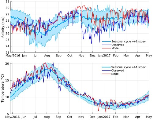
The FVCOM simulation covered the full annual cycle of May 2016 to April 2017, a time period chosen to provide the largest set of biological data to initialize and evaluate the follow-up biogeochemical model. Regardless of the particular choice, there will always be the question of how representative that period is in terms of capturing typical seasonal processes. From the physical perspective, Fig. 3 attempts, at least partially, to address that issue by superimposing sea surface salinities and temperatures observed at the Chrome Island lighthouse (see Fig. 1 for location) for May 2016 to April 2017 on curves of the average, and average plus/minus one standard deviation, computed over its complete observational period of 1961 to 2019 (model simulation values are also shown and will be discussed later). Though not consistently within one standard deviation of the long-term average, the cumulative time when the observed 2016–17 salinity curve is outside this band is considerably less than when it is inside with a significant drop from 29 to 25 psu in early November being notable. The 2016–17 temperatures are also generally within one standard deviation of the long-term average, though the steep drop from 20.3 °C on August 18 to 11.8 °C on September 6 is also notable.

Fig. 3 Chrome Island observed and modelled sea surface salinity (top) and temperature (bottom) for May 2016 to April 2017 superimposed on the average seasonal cycle plus/minus one standard deviation.

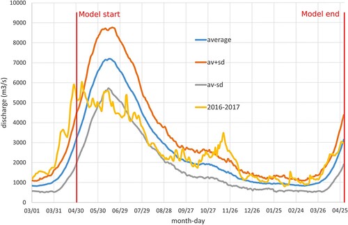
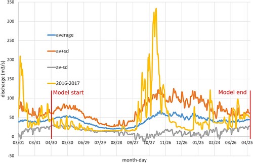
Fig. 4 provides another perspective of the representativeness of our simulation period by showing the average, average plus/minus one standard deviation, and 2016–2017 Fraser River discharges at Hope. The former three values were computed over the period of 1912 to 2019. These discharges can be viewed as a proxy for the volume of low salinity water in the southern SOG that could potentially enter into Baynes Sound, primarily from the south. The 2016–17 values are generally seen to be considerably larger than average prior to mid-May, lower than average from June through August, considerably larger than average in November, and generally within one standard deviation for the remainder of the simulation period. The fact that the discharges in March and April 2016 are beyond one standard deviation of the average suggests more freshwater, and lower than normal salinity, in the SOG at the beginning of our simulation.

Fig. 4 Average, average plus/minus one standard deviation, and March 1, 2016 to April 30, 2017 Fraser River discharges at Hope.

However, as the Fraser has a very large watershed, its discharge reflects both distant and local influences. A better indication of local freshwater influences is the Puntledge River which joins with the Tsolum River to become the Courtenay River just upstream of where it enters northern Baynes Sound. Given the influence of Courtenay River’s substantial freshwater contribution to Baynes Sound circulation, Waldie (1952) neglected the effect of all other streams except in their immediate vicinity of their estuaries. The Courtenay River’s discharge time-series data extends from 1914 to 2019 and in this case, the 2016–17 values (Fig. 5) show average or considerably larger than normal discharges prior to beginning of the model simulation (consistent with the Fraser), less than normal discharge between May and September followed by five storm events in October and November that, in the middle three instances, resulted in discharges well above normal. As discharges for the Englishman River (shown later), which lies south of the southern Baynes entrance (Fig. 2) but still within the model domain, show similar peaks in March 2016 and October 2016 through February 2017, we can conclude there were similar runoff patterns all along the eastern Vancouver Island coastline. Puntledge discharge was below average in December/January but close to normal from February to April, with the exception of a small storm in late February. These freshwater discharges and the resultant lower-than-normal salinity may influence Baynes’ ecosystem productivity through new nutrient inputs.

Fig. 5 Average, average plus/minus one standard deviation, and 2016–17 Puntledge River discharges just above its confluence with the Tsolum River just north of Courtenay.

A caveat should be noted in comparing these 2016–17 discharges with long-term statistics since the latter are not stationary due to climate change. For example, the Fraser River hydrograph has been shown to be flattening and have a peak that is arriving earlier in the year (Morrison et al., 2002). Analogous changes may be happening around Baynes Sound, as climate projections for coastal B.C. typically forecast wetter winters and dryer summers (e.g. Morrison et al., 2014). It is important to note that the summer of 2016 experienced record-breaking drought (Stage 4) and forest-fire conditions across the Sunshine Coast, within the Baynes Sound watershed, and the B.C. southern mainland influencing the Fraser River outflows (https://news.gov.bc.ca/releases/2016FLNR0134-001158). Though this issue certainly warrants further research, it is beyond the scope of the present investigation.

Temperature, salinity, and oxygen measurements have been taken over the entire water column at as many as forty stations in the Baynes Sound region since 2009 (Fig. 1 presents stations 1–38). Figs. 6 and 7 show the temperature and salinity profiles for April and June, the most frequently visited months, at stations BS2 and BS17 (Fig. 1), which are respectively located in the northern and southern ends of the Sound. These stations represent two distinct water masses influenced by spring river freshet (BS2) and tidally-induced mixing at the southern entrance (BS17). As 2016 is seen to be the freshest and warmest April at both stations, it would seem that water properties at the beginning of our model simulation period were quite anomalous. Certainly, the low salinities are consistent with the discharges seen in Fig. 5. The second freshest April is seen to be in 2017, at the end of our simulation, where the associated temperatures were “average”.

Fig. 6 Salinity and temperature profiles at CTD stations BS2 (left panels) and BS17 (right panels) for April.

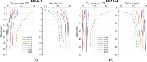
Fig. 7 Salinity and temperature profiles at CTD stations BS2 (left panels) and BS17 (right panels) for June.

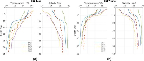
By June 2016, with the exception of the temperatures below 15 m at BS17, all temperature and salinity profiles are seen (Fig. 6) to be well within the envelope of profiles for other years. So, within two months, the anomalous April water properties had reverted back to “normal”, at least as determined by our limited observational set. However, as indicated by the anomalously fresh salinity profiles noted previously for April 2017 (Fig. 6), and perhaps as a lingering effect of the strong river discharges that arose in October and November 2016 (Figs. 4 and 5), this normality did not persist. And though beyond the end of our simulation period, Fig. 7 suggests that Baynes Sound remained anomalously fresh through to June 2017. In summary, over the duration of our model simulation period Baynes Sound was generally fresher than normal and had either normal, or warmer than normal, temperatures.

In general, the circulation pattern in Baynes Sound changes with the prevailing winds, river discharges, and inflows/outflows along the southern and northern entrances. Harmonic analyses of model output over the period of May 1 to October 31, 2016 produces an average sea surface topography (not shown), which indicates that there are weak geostrophic surface currents to the south throughout Baynes Sound. This scenario is consistent with river plumes discharging along Vancouver Island turning to the right. Waldie (1952) also documented the influence of the Courtenay River freshwater discharge that created tongue flows in a southern direction at a considerable distance along Denman Island.

3 FVCOM evaluations

Comparisons between hydrodynamic model output and observations are typically used to evaluate model accuracy, with the understanding that though there can be errors in (or problems with) the observations (an example is given later), they are generally accepted to reflect the truth. Fortunately, there are considerable data that can be used to evaluate the accuracy of our model simulation from May 1, 2016 to April 30, 2017. Those presented here will be restricted to comparisons of i) temperature and salinity, ii) currents; and iii) sea surface (predominantly tidal) elevation, as they will be the physical variables most affecting shellfish aquaculture.

a Temperature and salinity comparisons

Fig. 3 plotted observed and model sea surface salinities and temperatures at the Chrome Island lighthouse. Though there are only a few instances when the model temperatures missed observed warming or cooling events, relatively large salinity discrepancies are seen over the period of November to mid-December 2016, and to a lesser extent thereafter through to March 2017. Much of this can be attributed to the Englishman as well as Little and Big Qualicum Rivers not being included in our simulation and their freshwater discharges (analogous to those shown in Fig. 5 for the Puntledge) not affecting the model salinities at Chrome Island. Average root mean square (RMS) differences over the entire yearly simulation were 1.46 psu and 1.01 °C, respectively, with the largest salinity discrepancies arising in November and the largest temperature discrepancies arising in July.

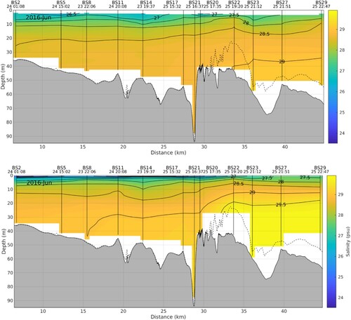
Figs. 8 and 9 compare observed and model temperature and salinity profiles at standard CTD stations along the central axis (Fig. 1) of Baynes Sound. Values from the June 2016 survey are shown here but similar plots are also available for April 2016 and April 2017 (Figs. S1 to S4), the only other months which had cruises during the model simulation period. As the April 2016 values were combined with other CTD observations to establish initial conditions for the model simulation, those model profiles are in close agreement with the observed. However, with the exception of slightly cooler values at depth beyond the southern entrance (stations BS22, BS23, BS27 and BS29), the June 2016 model temperatures are seen to be slightly warmer than those observed. Note that BS22 is close to the Chrome Island lighthouse and Fig. 3 showed the model sea surface temperatures (SSTs) to be too warm and the model sea surface salinities (SSSs) to be too fresh in late June. Though the near-surface model salinities are in reasonable agreement further to the north, they are slightly too salty at depth, especially beyond the southern entrance. Overall, the salinity and temperature discrepancies are less than 1.0 psu and 1 °C respectively, comparable to the RMS values at the Chrome Island lighthouse. We suspect they arise from a combination of i) inaccuracies in both the vertical and horizontal mixing and ii) the bathymetric smoothing that FVCOM requires to avoid instabilities and/or spurious currents. As seen in the June 2016 (Figs. 8 and 9) and April 2017 (Figs. S3 and S4), the model flow below 25 m over the sill at the southern entrance to Baynes Sound is blocked. This sill was shallowed in the model during the bathymetric smoothing. As the model was used in the subsequent biogeochemical modelling for aquaculture assessments, it was important to preserve the near-by shallow depths and mudflats. By not allowing the mudflats to become deeper during the smoothing, depths in the channel became shallower.

Fig. 8 Temperature profiles observed at CTD stations along the Baynes Sound thalweg during the June 2016 survey (upper panel) corresponding model values (lower panel) at the same locations and time. Station names, dates, and times for each CTD cast are at the top of each panel. Model values were interpolated to coincide with these times. The dashed line is the bottom profile from the model bathymetry, while the grey shaded region denotes the true bathymetry.

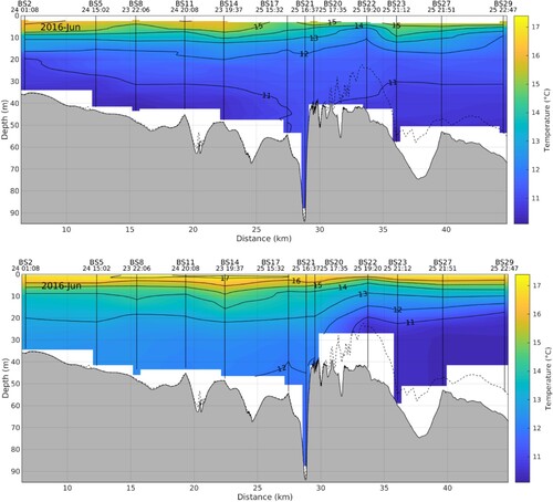
Fig. 9 Salinity profiles observed at CTD stations along the Baynes Sound thalweg during the June 2016 survey (upper panel) and corresponding model values (lower panel) at the same locations and time. Station names, dates, and times for each CTD cast are at the top of each panel. Model values were interpolated to coincide with these times. The dashed line is the bottom profile from the model bathymetry, while the grey shaded region denotes the true bathymetry.

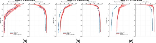
Whereas the analogous thalweg plot for April 2017 (Figs. S3 and S4) indicates that the model temperatures were generally too warm and the salinities too salty, Fig. 10 allows a more precise indication of model versus observed discrepancies. It shows profiles at station BS17 in central Baynes Sound for April and June 2016, as well as April 2017. As mentioned above, the April 2016 agreement is quite good because the observations were used to establish initial conditions for the model simulation. The observed temperature profile is seen to lie within the model envelope of daily variations while the corresponding observed salinities fall below the envelope (i.e. the model is too salty) by a maximum of about 0.5 psu near the surface and below 20 m depth. The June 2016 model temperatures are seen to be too warm by at most 1 °C while the associated salinities are too salty by at most 0.4 psu. Finally, the April 2017 profiles show the model temperatures again being approximately 1 °C too warm and the model salinities being approximately 0.6 psu too salty, both of which are consistent with the SST and SSS discrepancies seen for this time at Chrome Island (Fig. 3).

Fig. 10 Observed and model temperature and salinity profiles at CTD station BS17 for April and June 2016 and April 2017 from left to right panels (see Fig. 1). The thick red lines indicate model values at the time of observation while the thin red lines are at 20 min intervals over the day, thus providing an indication of variations over a tidal cycle. Note the different scaling on the x-axes.

The degree to which FVCOM captured observed temperatures and salinities in Baynes Sound is generally comparable to what HCC03 found with their model. Although the initial accuracy of their 2-km Strait of Georgia model was limited by taking April 2002 initial salinities and temperatures from 1968 when the Fraser River discharges for January to March were approximately double those in 2002, these discrepancies changed with the application of their atmospheric, Fraser, and Courtenay River forcing. By June 7, the model and observed temperatures in Baynes Sound were very close, both in terms of actual values and correctly capturing the observed stratification, but the model had become too salty by approximately 1–1.5 psu. As the simulation progressed to August 27 and September 17, times of the next surveys, the salinity discrepancy decreased slightly but model temperatures became too warm seemingly because cold water bottom intrusions from the Strait of Georgia were not reproduced correctly, analogous to that seen in Fig. 8a and b.

Similar to the daily SST and SSS observations taken at the Chrome Island lighthouse, temperatures and salinities were also observed (with 10-minute sampling and at approximately 5 m depth) at five other sites within or near Baynes Sound (see the yellow triangles in Fig. 1) for at least part of the model simulation period. As illustrated in Fig. 11, there is generally good agreement between the model and observed temperatures, in terms of capturing both actual values and variations in time. For example, the Coefficient of Determination (R²) between modelled and observed data are as follows: Comox Marina (R² = 0.91234); Fanny Bay Dock (R² = 0.90379); Hornby Island Terminal (R² = 0.77633); Lucky Seven (R² = 0.86549); Mac’s Oysters (R² = 0.88739). However, the agreement is uniformly much poorer for the associated salinities (not shown) and much of that can be attributed to bio-fouling of the measurement devices.

Fig. 11 Observed and modeled temperatures at the five sites (Comox Marina, Fanny Bay Dock, Hornby Terminal, Lucky Seven, Mac’s Oysters) shown with yellow triangles in Fig. 1.

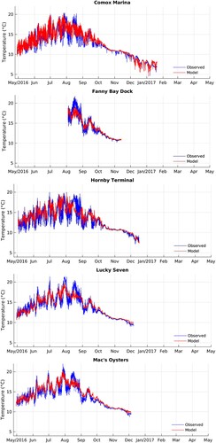
The model underestimates the amplitude of several cold and warm events in July and August into varying degrees at the five probe stations and at the Chrome Island lighthouse. The exact cause of this is unknown, but we speculate that the model may lack the advective capability to transfer anomalies from the southern open boundary during this time. Indeed, the beginning of August and beginning of September cold anomalies are seen in the southern open boundary temperature forcing. However, the mid-August warm anomaly is not stronger at the open boundary than the model values at the observation sites. Overmixing in the model can contribute to these discrepancies as well. However, the mid-August warming is not seen in the air temperature forcing, either which is another possible cause of the missed warm peak in the model water temperature.

b Current velocity comparisons

Unfortunately, there are not many current meter observations in Baynes Sound that can be used to evaluate the accuracy of our model currents. Though four ADCPs were deployed at different times and locations, instrument failures at two made their data largely unusable. The two successful deployments were carried out by 1) Cascadia Coast Research (Clayton Hiles, personal communication, 2014) under contract to BC Ferries for the period of February 25 to April 12, 2012; and 2) DFO (in support of this project) in Union Bay for the period of June 15 to August 30, 2016 (Fig. 1). Both successful deployments were upward-looking bottom moorings with the first having hourly observations over the range of 38.5 to 1.5 m in 1 m intervals, and the second having 5-minute sampling over the depth range of 11.1 to 2.1 m in 1 m intervals.

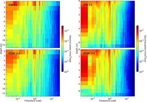
Though an ADCP typically measures currents in terms of orthogonal coordinates (e.g. east–west and north–south components), those currents can equivalently be expressed in terms of counter-rotating vectors, one rotating clockwise and the other counter-clockwise. The left panel of Fig. 12 adopts this convention in displaying the power spectra versus depth for the entire time series of the BC Ferries mooring. The clear vertical band at approximately two cycles per day is due to the semi-diurnal tides while the weaker band around one cycle per day arises from the diurnal tides. However, the most noteworthy feature in both rotary spectra is that most of their energy is in frequencies lower than daily, which would have been forced by variations in a combination of winds, river discharges, and inputs from the SOG. This low frequency energy is seen to be largest near the surface (predominantly from the winds and discharges) and smallest between 20 and 25 m depth, which is the interface between the two layers of estuarine flow (outward toward the SOG near the surface and inward from the SOG below) that exist in Baynes Sound. (This estuarine feature will be described in more detail later.)

Fig. 12 Rotary spectra versus depth at the BC Ferries ADCP mooring location over the period of February 25 to April 12. Left panels are for the observations in 2012 while the right panels are from the model simulation in 2017. CW and CCW denote clockwise and counter-clockwise components, respectively. Note the frequency axis and power colour legend have logarithmic scaling. Depth is relative to mean sea level.

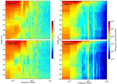
The right panel of Fig. 12 also displays rotary spectra computed over the period of February 25 to April 12 but for the model simulation in 2017. Acknowledging that there will be differences solely because of the different years, the model spectra do show many of the same features as those computed from the observations. The model has somewhat more energy near the surface and less energy at higher frequencies. But the relatively small energy in the tides, the much larger energy at low frequencies, and minimal energy in the 20 to 25 m depth range indicate the model has done a reasonable job of capturing the current spectra at this location and for this time of the year. Fig. 13 presents a similar comparison for currents at the Union Bay site over the period of June 15 to August 30, 2016. In this case, tides in the left panel are seen to account for a relatively larger proportion of the power and to be larger near the surface. However, significant energy still exists at frequencies below daily with more in the model currents than the observed. However, because this site is so shallow there is not a two-layer estuarine flow in this area. Mean flows at the Union Bay site over the observational period (not shown) are toward the north-northeast and range from a maximum of approximately 1.6 cm s⁻¹ at 4 m depth to 0.2 cm s⁻¹ near the bottom. The model shows similar mean flow profile at this site (not shown), albeit with maximum flow reaching 4 cm s⁻¹. The stronger model flow is consistent with the shallower model bathymetry at this site and the model attempting to preserve the flow volume.

Fig. 13 Rotary spectra versus depth at the Union Bay ADCP mooring location over the period of June 15 to August 30, 2016. Left panels, from observations; right panels, from the model simulation. CW and CCW denote clockwise and counter-clockwise components, respectively. Note the frequency axis and power colour legend have logarithmic scaling. Depth is respect to mean sea level.

Even though the tides comprise a relatively small proportion of the total current energy at the BC Ferries site, traditional harmonic tidal analyses were performed to compute the observed and model current ellipses over the water column. The coherent tidal energy portion of the total energy budget of the observed currents at the BCF location ranges from 9% near the surface and the bottom to 37% near 20 m depth. At the Union Bay location, it has two maxima of 32–35%, near the surface and at 6–8 m depth, and two minima at 4 m depth and close to the bottom at 10 m depth. These numbers are based on the February to April 2012 deployment at the BCF location (∼44 days) and the July 29 to August 30, 2016 deployment at Union Bay (∼32 days).

The model shows similar vertical distribution of tidal energy percentage for the periods matching the observations. At the BCF location, the tidal energy constitutes 3% of the total current energy at the surface, increasing to 47% at 22 m depth and then falling off to 26% at the bottom. At the Union Bay location, the model shows two maxima of 45–47%, one at the surface and another near 4 m depth, and two minima, at 2 m depth and at the bottom (the model bottom depth is 6.5 m at this location).

As the current vector for each tidal constituent traces out an elliptical pattern over its period, the ellipse parameters (major and minor axes lengths, orientation, and vector position at the time of maximum tidal potential forcing) provide a commonly used framework for characterizing tidal currents. The left-most column of Fig. 14 shows how the observed M2 (top) and K1 (bottom) ellipses vary with depth. Note that due to acoustic contamination, observations are not reliable near the surface, so the uppermost values only go to 2 m depth. However as tidal currents can vary seasonally, the next four columns show analogous ellipses arising from harmonic analyses of the model currents, specifically for the periods of JFM 2017 (January, February, March), MJ 2016 (May, June), JAS 2016 (July, August, September), and OND 2016 (October, November, December). Note also, that the observed ellipses are located at fixed distances from the bottom, while the vertical position of the model ellipses (located at mid-points of sigma-layers) varies with changes in sea surface height. As a result, the position of the near-surface model ellipses relative to the bottom undergoes tidal excursions of 2–3% of the water column height with such excursions for the near-bottom ellipses being negligible.

Fig. 14 Ellipses versus depth at the BC Ferries ADCP location: upper panel for M2 and lower panel for K1. The left-most column was computed from the observations over the period of Feb 25 to Apr 12, 2012, while the next four columns were computed from the model currents for the respective periods of JFM2017, MJ2016, JAS2016, and OND2016. Blue ellipses denote vectors that are rotating counterclockwise while red ellipses denote clockwise rotation.

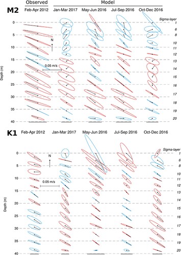
The K1 observed and model ellipses are generally seen to have similar eccentricity, orientation (both roughly aligned with the main axis of Baynes Sound), and magnitudes. Though the sense of rotation of the current vector within each ellipse often differs, this is only an important issue when the minor axes are large relative to the major, which is generally not the case here (eccentricity ratio is below 0.2 for the most depths). However, the considerable variation among the model phase lags (as designated by the black lines within each ellipse) is indicative of seasonal variations in ebb/flood timing associated with this constituent. The season with ellipses closest to those observed is JFM2017. However, agreement between the model and observed M2 ellipses is not as good, particularly in the upper 20 m. In the lower half of the water column, the best agreement is with the MJ2016 and JAS2016 values with ellipse errors (according to Cummins and Thupaki (2018)) between 0.010 and 0.015 m s⁻¹, when both sets of ellipses are reasonably consistent over that depth range. Considerable variations over the water column for the JFM model ellipses (i.e. baroclinic content) suggest that horizontal and vertical gradients in water density (e.g. salinity and temperature) were different in 2012 than 2017. Unfortunately, no CTD surveys were taken in April 2012, but Fig. 6 does show that salinities in April 2017 (and presumably JFM 2017) were fresher than normal. Though the Puntledge River discharges were comparable for JFM in 2012 and 2017 (not shown), the Fraser River discharges for JFM 2012 (also not shown) were considerably smaller than those for 2017. Therefore, it is reasonable to conclude that near surface water entering Baynes Sound from the SOG in 2012 was more saline and, thus, more likely to produce the barotropic ellipses seen in the left-most column of Fig. 14. A figure similar to 14 but for the ADCP at Union Bay has not been shown because model bathymetry has been significantly modified (smoothed) near the deployment location to ensure numerical stability of the simulation thus changing the local flow regime and preventing fair comparison between the model and observed currents.

c Sea surface elevation comparisons

As a proxy for assessing the accuracy of the tidal elevations within the model, Table 1 compares observed and model amplitudes and phases (harmonics) for the five constituents specified in the model boundary forcing. The semi-diurnal and diurnal constituents have periods around twelve and twenty-four hours respectively, with the largest, M2 and K1, having periods of 12.42 and 23.93 h respectively. This comparison is done at five tide gauge stations (Fig. 2a) within the model domain and with the model values calculated from the simulation that included wetting-and-drying mudflats in the FVCOM dynamics (shorter simulation without wetting-and-drying showed little change to the model harmonics). The observed harmonics were taken from Canadian Hydrographic Services data archives and are based on analyses of historical data, as none of these sites were active during the model simulation period. The closest active sites are Campbell River and Point Atkinson, both of which are just outside our model domain. Though the model amplitudes are consistently within 2 cm of their observed counterparts, some of the associated phase differences are as large as 10.9°. (Note, for semi-diurnal constituents a 5° phase difference translates to high/low water being out by approximately 10 min while for the diurnals, a 5° difference translates to a 20-minute error). This is because boundary forcing for the M2 and K1 constituents were taken directly from Foreman et al. (2004), while analogous values for constituents S2, N2, and O1 were estimated using amplitude ratios and phase differences based on harmonic analysis results for the Comox tide gauge. Though the results are not shown here, a sensitivity run with no wetting and drying of the mudflats (i.e. a minimum depth was set so that mudflats never became dry) made little difference to the model accuracy. Assuming the mudflats in our model are adequately represented, this indicates that even though there are extensive mudflats in Baynes Sound, they play a minor role in the overall regional tidal dynamics. In fact, Dupont et al. (2005) show (their Fig. 7) that the average frictional dissipation over the mudflat region of their Bay of Fundy model is a very small proportion of the total dissipation. Assuming a dissipation figure for Baynes would be similar, this would explain why our runs with and without mudflats showed very little change to the amplitudes and phases at our tide gauge sites. Additonally we note, that the difference between the volume of water in Baynes Sound in the model with wetting/drying and the model with a minimum depth of 4 m is only 2.3%.

Table 1. Comparison of observed and model amplitudes (m) and phases (degrees) at five tide gauge locations (Fig. 2a) and Union Bay ADCP location (Fig. 1). RMS values were calculated using equation 3 in Cummins and Oey (1997). The asterisked (*) constituents were inferred due to insufficient length of the analyzed time series.

Station	Constituent	Observed		Model
						Discrepancy with observation		RMS
		Amp	Phase	Amp	Phase	Amp	Phase	Abs	Rel (%)
Comox	O1	0.489	264.6	0.484	272.8	0.005	−8.1	0.049	10.0
	K1	0.885	287.5	0.878	286.9	0.007	0.6	0.008	0.9
	N2	0.220	7.7	0.222	11.5	−0.002	−3.8	0.010	4.7
	M2	1.002	33.9	1.009	33.2	−0.008	0.7	0.010	1.0
	S2	0.253	62.6	0.256	53.8	−0.003	8.8	0.028	10.9
Little River	O1	0.496	263.6	0.484	272.6	0.012	−8.9	0.055	11.0
	K1	0.895	288.0	0.877	286.8	0.018	1.2	0.018	2.0
	N2	0.216	3.5	0.220	10.4	−0.004	−7.0	0.019	8.8
	M2	0.984	33.8	1.002	32.2	−0.018	1.6	0.023	2.4
	S2	0.250	63.8	0.254	52.9	−0.004	10.9	0.034	13.6
Hornby Island	O1	0.469	267.6	0.483	272.5	−0.014	−5.0	0.031	6.5
	K1	0.881	288.9	0.875	286.6	0.006	2.3	0.025	2.8
	N2	0.228	10.7	0.219	11.1	0.009	−0.4	0.007	2.9
	M2	0.982	36.5	0.994	32.8	−0.013	3.7	0.046	4.7
	S2	0.262	65.6	0.253	53.5	0.010	12.2	0.039	15.0
Irvines Landing	O1	0.483	263.8	0.484	271.9	0.000	−8.1	0.048	10.0
	K1	0.892	286.4	0.878	285.9	0.014	0.5	0.011	1.3
	N2	0.213	5.5	0.218	10.7	−0.005	−5.2	0.014	6.7
	M2	0.987	32.3	0.992	32.5	−0.005	−0.2	0.004	0.4
	S2	0.248	61.4	0.252	53.2	−0.004	8.2	0.026	10.3
Saltery Bay	O1	0.481	264.7	0.487	272.3	−0.006	−7.5	0.045	9.4
	K1	0.873	287.7	0.883	286.4	−0.011	1.3	0.016	1.8
	N2	0.226	5.7	0.223	11.4	0.003	−5.6	0.016	7.0
	M2	0.996	32.9	1.014	33.1	−0.018	−0.2	0.013	1.3
	S2	0.244	63.1	0.258	53.9	−0.014	9.2	0.030	12.4
Union Bay	O1	0.490	267.3	0.493	271.8	−0.003	−4.5	0.027	5.5
	K1*	0.838	289.6	0.759	275.9	0.079	13.7	0.145	17.3
	N2	0.176	2.9	0.223	12.0	−0.046	−9.1	0.040	22.4
	M2	0.970	33.1	1.010	33.5	−0.040	−0.5	0.029	3.0
	S2*	0.233	60.3	0.276	46.1	−0.043	14.2	0.054	23.0

In addition to the tidal constituents at the tide gauges, we have analyzed the pressure record from the ADCP instrument deployed in Union Bay. The length of the time series was 76 days, which prevented direct estimate of constituents with close frequencies. For K1-P1 and S2-K2 pairs we used inference based on their theoretical ratios of amplitudes and assumed zero phase differences. The corresponding model series was trimmed to the length of the observed series and analyzed in a similar way for consistency. The results (Table 1) show a better model performance at this location than for the tide gauges for O1, a similar performance for M2 and an inferior performance for K1, N2 and S2. For all five constituents, however, the amplitude differences are within 8 cm and phase differences are within 15°. The model de-tided sea level oscillations of 2–3 cm in amplitude are significantly smaller than the observed oscillations of 5–7 cm, and, although both have synoptic time scales, they are not correlated with each other (not shown). This suggests that the large part of non-tidal sea level variability should come to the domain through the lateral boundaries. However, taking into account the overall small observed non-tidal variability in the domain, we consider the absence of synoptic scale sea level forcing in our model not critical for the model physical processes and for the purposes of the subsequent biogeochemical modelling.

4 Further analysis of the oscillations in the four temperature time series

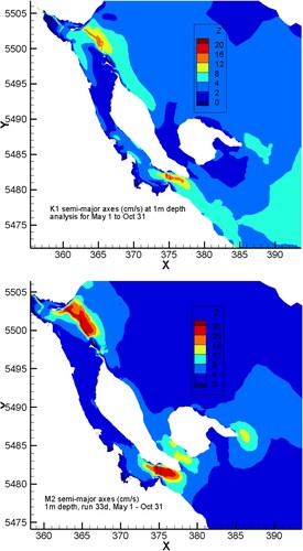
Fig. 15 shows the K1 and M2 major semi-axis currents at one-meter depth as calculated by a harmonic tidal analysis over the period of May 31 to October 31, 2016. The strongest currents are clearly seen at the northern and southern entrances to Baynes Sound and can be expected to have major impacts on tidal mixing and seabed sediment sorting and stability in these regions (Sutherland et al., 2018; Sutherland & Amos, 2020). As the S2 currents are approximately 40% of M2, there should also be a notable spring-neap cycle in this mixing and in fact, this seems to be evident in the temperature times series displayed in Fig 11. For example, Fig. 11 suggests that the temperature oscillations at the Mac’s Oysters site are generally consistent with the spring-neap tidal cycle over June through August. Although the daily range in tidal height (as computed by FVCOM at nearby model node) is used as a proxy for this cycle, it should be noted that tidal mixing varies with the velocity rather than height and this could accentuate the relative magnitude of the highs and lows to more closely capture the larger changes seen in the water temperatures. However, the winds also play a role as the largest water temperature peak in late July corresponds with relatively strong (4 m s⁻¹) winds from the northwest. Although there are times (e.g. early June) when warmer air temperatures lead and are likely to explain the rise in water temperature, there are other times when peaks in the water temperature must be influenced by other factors. Certainly, there are many instances where dips in air temperature do not cause similar dips in the water temperature.

Fig. 15 K1 (top) and M2 (bottom) semi-major axes at 1-metre depth as calculated from harmonic analysis of model currents for the period of May 1 to October 31, 2016.

In order to further explore the observed and model water temperature oscillations at synoptic/fortnightly time scales, a multivariate linear regression analysis (partial least squares, PLS) is performed using daily tidal range (as a proxy for the spring-neap cycle), air temperature and wind speed as predictors. As an example, Fig. 16 shows the observed water temperature and the corresponding predictor time series at the Mac’s Oysters site. All variables are taken at same location (i.e. tides from FVCOM and atmospheric variables from HRDPS) and resampled to daily values. Wind is rotated along the semi-major axis of variance which largely corresponds with the along-shore direction, e.g. the along shore component of wind at Mac’s Oysters is positive towards −35°T (325°T). The cross-shore component (along the semi-minor axis) is seen to be small in Fig. 16 and is ignored in the following calculations.

Fig. 16 Observed water temperature, model daily range in sea surface elevation, and air temperature and wind components along and cross the axis of Baynes Sound from HRDPS at Mac’s Oysters site for the period of May to November 2016.

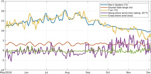
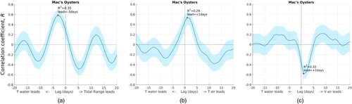
Strong oscillations at synoptic/fortnightly frequencies are observed in T_water (water temperature) during summer season only (July to September). During other months, changes in temperature are small so we restrict this analysis to summer months. Thus, T_water and T_air (air temperature) have strong seasonal component which we remove by applying a high-pass filter at 40-day cut-off before calculating correlations. The lag which produces the highest absolute value of the correlation between the predictor and T_water is determined (Fig. 17). For all three predictors the maximum correlation magnitudes are similar, with wind correlation being negative meaning positive anomalies in the observed T_water occur when the wind blows from the northwest. T_water lags T_air and wind by 1 d and leads the maximum spring tide by 3 days, as seen in Fig. 17.

Fig. 17 Lag time relationships between observed water temperature and i) tidal range (left graph), ii) air temperature (middle graph), and iii) wind (right graph).

The next step is to apply PLS analysis to calculate multivariate regression between T_water and the predictors shifted in time to account for the lag calculated above. The results are presented in Table 2 with the exception of the Fanny Bay three-month time-series, that was deemed to be too short for the analysis.

Table 2. Partial least squares regression of the observed and the model water temperature on the diurnal tidal range, air temperature, and wind speed at CTD probe stations: Predictor lead/lag period (days) and associated coefficient of determination (r²).

Station/Predictor	Predictor lead (+)/lag (−)		Total r^2		Partial r^2		Individual r^2
	Obs	Model	Obs	Model	Obs	Model	Obs	Model
Comox Marina			0.59	0.45
Tidal Range	6	−3			0.11	0.01	0.28	0.15
T air	1	1			0.13	0.05	0.28	0.15
V air	1	2			0.13	0.24	0.30	0.36
Hornby Terminal			0.56	0.27
Tidal Range	5	6			0.13	0.01	0.26	0.06
T air	1	1			0.08	0.10	0.19	0.18
V air	1	1			0.16	0.07	0.35	0.14
Lucky Seven			0.61	0.50
Tidal Range	−3	−2			0.11	0.04	0.34	0.23
T air	2	2			0.11	0.11	0.27	0.27
V air	2	2			0.13	0.14	0.32	0.29
Mac’s Oysters			0.60	0.49
Tidal Range	−3	−3			0.09	0.04	0.34	0.21
T air	1	2			0.08	0.13	0.28	0.27
V air	1	2			0.15	0.12	0.33	0.27

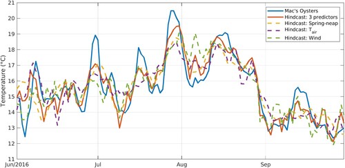
Individual skill in Table 2 is the variance explained by a single predictor on its own and this corresponds with the skill (R²) in the lagged correlation plots. Partial skill shows how much the model skill is improved by adding this predictor to the rest. For Mac’s Oysters, the tidal cycle and T_air improve the regression by a similar amount, adding 8–9% to the explained variance. The along-shore wind produces a higher improvement of 15%. The difference between the individual and partial skill is due to an inter-correlation of the predictors. Partial skills significantly lower than individual skills in our case indicate a high degree of mutual correlation between the predictors. The three predictors combined explain 60% of the variance in the observed T_water. For the model T_water, the regression skill is lower and ranges between 0.27 and 0.50 with diurnal tidal range explaining less variance than for the observed series consistently across at all stations. The hindcast water temperature series generated with the above regression are shown in Fig. 18. The seasonal signal that was subtracted prior to calculating the regression coefficients has been added back in this plot. In addition to the hindcast obtained from all three predictors (solid red line), hindcasts from individual predictors are also shown (dashed lines). No single predictor seems to be distinctly better than others, suggesting that each predictor plays an important role at different times. Note that at least part of the remaining unexplained variance could be due to nonlinear relationships. For example, as the wind influence is expected to be through the stress, it should vary quadratically. Other factors influencing water temperature may include non-local warming/cooling in combination with advection. Although the local wind is, in part, responsible for the surface currents, it does not reflect the entire complexity of the advective mechanism for Mac’s Oysters.

Fig. 18 Observed water temperature at the Mac’s Oysters location along with hindcasts based on regressions with each and all of the spring-neap tidal cycle, air temperature, and along-shore wind as predictors.

5 Volume fluxes in/out of Baynes Sound

The FVCOM currents produced over our yearly simulation can be used to estimate seasonal volume fluxes into and out of Baynes Sound. Figs. 19 and 20 show average velocity profiles along transects (Fig. 2b) crossing the northern and southern entrances to the Sound for the four seasons: spring (April-May-June), summer (July-August-September), fall (October-November-December), and winter (January-February–March). Table 3 quantifies the associated volume fluxes (including a partition of outflow versus inflow along with the combination) and includes river input so that overall balances can be estimated. (Note that the incoming/outgoing fluxes do not perfectly add to the combined values because slightly different approaches were used in their respective calculations). Two-layer estuarine flows (outflow at the surface, inflow at depth) are consistently seen at the southern entrance and in the northern (deeper) portion of the northern entrance. Note that the large outgoing volume flux at the northern entrance is generally restricted to the top 5 m (approximately; Fig. 19), while at the southern entrance it is between the top 5 and 35 m (Fig. 20). Sloping of the 2-layer system at the southern entrance is due to the Coriolis force wherein flows are pushed to their “right” in the northern hemisphere and to the “left” in the southern hemisphere. Similar slopes are also seen in the two-layer flows in Juan de Fuca Strait and Queen Charlotte Strait.

Fig. 19 Average velocity (m s⁻¹) profiles along a transect (Fig. 2b) crossing the northern entrance to the Sound for the four seasons: spring (April-May-June), summer (July-August-September), fall (October-November-December), and winter (January-February-March). Red = incoming, blue = outgoing, y-axis is depth (m), x-axis is transect distance (m), measured from Denman Island.

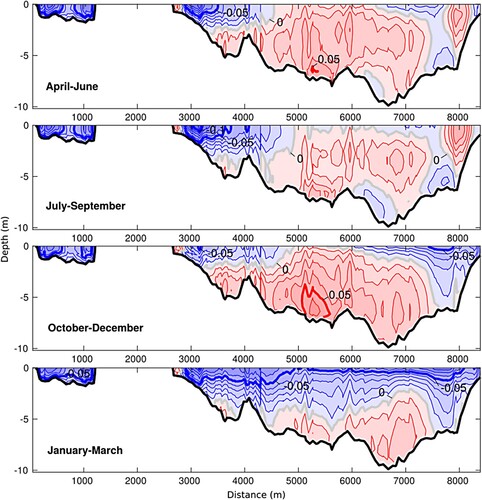
Fig. 20 Average seasonal velocity (m s⁻¹) profiles across a transect at the southern entrance to Baynes Sound (see Fig. 2b for transect location). X-axis is distance measured from Vancouver Island. Red = incoming, blue = outgoing.

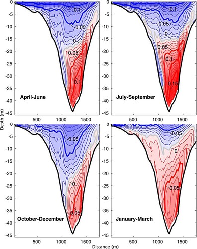
Table 3. Average seasonal volume transports (m³s⁻¹) crossing the northern and southern entrances to Baynes Sound, and estimated balances corresponding to the velocities shown in Figs. 20 and 21. AMJ = April, May, June; JAS = July, August, September; OND = October, November, December; JFM = January, February, March.

Season	North			South			Rivers	Balance
	inflow	outflow	net	inflow	outflow	net
AMJ	545	−321	224	566	−870	−304	67	−13
JAS	277	−393	−116	827	−757	70	33	−14
OND	646	−270	376	305	−778	−473	84	−13
JFM	177	−693	−516	690	−267	423	80	−12
Year	412	−418	−6	596	−670	−73	66	−13

The relative magnitude of outflow versus inflow is seen (Table 3) to not only fluctuate seasonally, but also between the two passages, i.e. one entrance is not consistently the conduit for inflow or outflow (Note that the volume transport estimates have been filtered to remove the tides). Except inflow in the fall and outflow in the winter, the larger fluxes are seen to be via the southern entrance. The relatively small, and consistently negative, seasonal imbalances can likely be attributed to a combination of i) model velocity output being 20-minute snapshots rather than averages over each time interval, ii) the FVCOM numerics not conserving volume perfectly, and iii) averaging errors arising when calculating the volume flux.

6 Water renewal time

In the context of carrying capacity assessments for shellfish aquaculture, water renewal or flushing is a key feature of coastal ecosystems providing an indication of the hydrodynamic capacity of the system to renew shellfish food through exchange and mixing. FVCOM outputs were combined with a passive numerical tracer to compute the spatial distribution of water renewal time (WRT) over BS following Koutitonsky et al. (2004). In brief, a passive tracer was introduced with an initial concentration C = 1 (arbitrary units) within BS, C = 0 everywhere else and forced to C = 0 at the river and open boundaries. This tracer was then transported and exchanged following the same advection–dispersion scheme as for temperature/salinity. Any location within BS was deemed renewed when the tracer concentration fell below 1/e (∼ 37%) of its initial value (e-folding renewal time). Therefore, the WRT corresponds to the time needed for the water initially located at a specific location within the Sound’s 3D space to be renewed by water coming from the outside, i.e. either from the SOG or from river run-off. Fig. 21 presents the WRT distribution in both the surface and bottom layers of the BS model. We can expect the variation in WRT over the tidal cycle to be a matter of hours, which would not change substantially the reported values of WRT, except for limited areas in the vicinity of the Sound’s entrances. Moreover, these WRT estimates were provided in the context of the general description of Baynes Sound’s hydrodynamics and as a comparison point with the HCC03 study.

Fig. 21 Spatial distribution of water renewal time (WRT) in the surface (left) and bottom (right) layers of Baynes Sound.

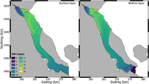
Overall WRT estimates in the 10–16 d range are consistent with the 15.8 d value reported by Hay and Co (2003) using a similar method but integrated through space. Although the WRT is influenced by the conditions prevailing at the time of the beginning of the simulation (1 May 2016), it can still provide insight in the main water circulation characteristics of BS. The surface layer results show the limited influence of the Courtenay River discharge and other smaller rivers. Moreover, WRT tends to increase from south to north in both the surface and bottom layers, which is consistent with the southern entrance showing the largest net exchange on a yearly basis, although tracer releases on other dates confirm that the WRT fluctuates both seasonally (as expected from Table 3) and with the particular conditions over the approximately fifteen-day flushing period. This result and the generally shorter WRT in the bottom layer highlight the importance of the two-layered estuarine circulation for the overall BS water circulation and renewal.

7 Summary, discussion, and future work

The foregoing presentation has detailed the development and evaluation of a circulation model for Baynes Sound. The intent was to update the earlier modelling efforts of Hay et al. (2003) with a newer model, FVCOM, whose grid has a finer spatial resolution and whose dynamics incorporate the wetting and drying of tidal flats. This model was forced with wind and heat flux values from the HRDPS 2.5 km atmospheric model, discharges from four rivers, and outer boundary elevations from observations and larger domain models. A simulation was carried out for the period of May 2016 to April 2017 and analyses were presented to characterize the Baynes Sound salinity, temperature, and river discharges for that time period in the context of long-term statistics. In general, salinities were seen to be fresher than normal while temperatures were either normal, or warmer than normal.

Model results were compared with CTD, ADCP, and sea surface height (SSH) observations and generally found to be in reasonable agreement. An experiment wherein the mudflat wetting and drying was replaced with a minimum depth that does not allow drying demonstrated that although the low-tide mudflats are extensive, they only make a small difference to the regional tidal dynamics, consistent with the energy dissipation finding of Dupont et al. (2005) in the Bay of Fundy. Tidal energy contribution at various locations towards the total observed SSH energy is as follows: 1) Little River: 98.0%; 2) Hornby Island: 98.6%; Irvines Landing: 98.8%; and Saltery Bay: 99.2%. The estimates are based on historical data, where none of the observed series overlaps with the simulation period. For the model, the tidal contribution is 99.9% at all tide gauges due to absence of synoptic SSH forcing. Non-tidal oscillations at synoptic time scales in the model are an order of 2 cm in amplitude, while in the observed series they are in the order of 5–7 cm. The standard deviation of the observed non-tidal SSH during summer months is 0.1, while during winter months it is 0.2 m. A multivariate linear regression analysis was carried out to determine the extent to which oscillations in near-surface temperature at four locations around Baynes Sound were dependent on the spring-neap tidal height range (a proxy for tidal mixing), air temperature, and along-sound wind velocity. No single predictor was found to be consistently better than the others, suggesting that each plays an important role at different times.

The model was used to estimate seasonal volume fluxes across the northern and southern entrances to the sound. Both transects showed two-layer estuarine flows wherein, with the exception of inflows in the fall and outflows in the winter, the larger fluxes were found to be through the deeper southern entrance. Water renewal times throughout the sound were also estimated and found to increase from south to north in both the surface and bottom layers; a result consistent with the southern entrance having the largest net exchange on a yearly basis.

Discharges for the Englishman and Little Qualicum Rivers (see Fig. 2 for locations) for the period of January 1, 2016 to April 30, 2017 are shown in Fig. 22 and seen to be very small from the beginning of the model simulation on May 1 until early October. Only after that time would several storms have provided significant freshwater to the SOG south of Baynes Sound. Though its mouth is closer to the southern entrance of Baynes Sound, the Big Qualicum River only had its discharges measured by Water Survey of Canada for years 1913 to 1974 (albeit with many gaps) and thus they are not available for the simulation time period. However, a dam and sluice gate control the flow of this river from Horne Lake and a comparison of lake outlet flows with those at the ocean mouth over the period of 1958 to 1962 show the former to be only slightly less than the latter. Furthermore, a plot comparing the 1964 to 1974 discharges at the river mouth with those for the Little Qualicum River shows the latter to be approximately three times larger over the months of October to March. (Unfortunately, very few Englishman River discharge measurements were available over the same time period). Assuming these relationships continued to our model simulation period, the Big Qualicum River would have contributed much less freshwater to the SOG south of Baynes Sound than the Little Qualicum and Englishman Rivers.

Fig. 22 Englishman and Little Qualicum River discharges (m³ s⁻¹) for the period of January 1, 2016 to April 30, 2017.

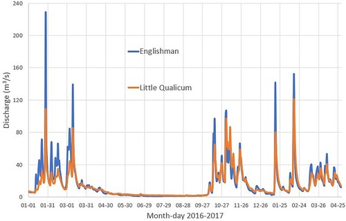
In all likelihood, repeating the FVCOM simulation with the inclusion of discharges from the Englishman and Little and Big Qualicum Rivers would improve the model versus observation salinity comparisons at Chrome Island (Fig. 3) between mid-October 2016 and early March 2017. To a lesser degree, it may also improve the temperature time series comparisons in Fig 11. However, from the perspective of the shellfish carrying capacity in Baynes Sound and the biogeochemical model that has been developed to assess it, this time period is relatively unimportant compared to the higher growth period of March through September. For example, phytoplankton populations dwindle, sink-out, and/or overwinter (resting spores) in the winter season between October and March. The fall diatom bloom, predominated by Skeletonema, Chaetoceros, ceases at mid-October in the SoG, while the spring bloom generally initiates in mid- to late March (Gower et al., 2013; Haigh et al., 1992, 1994; Haigh & Taylor, 1991; Sutherland et al., 2023). Limited light availability and cold temperatures during this winter period contribute to the reduction of phytoplankton productivity, regardless of river-based nitrogen sources that may augment limiting marine nitrogen sources associated with certain oceanographic scenarios (St. John et al., 1993). Moreover, incorporating these rivers would be a significant undertaking, requiring not only refinements to the grid near the three river mouths, but also re-aligning all the model forcing fields over the entire model domain. In light of these arguments, it was decided to leave the inclusion of these three rivers to future work.

Though not described here, the circulation model has been coupled to a biogeochemical model in order to update the shellfish carrying capacity conclusions presented by Hay et al. (2003). This objective placed constraints on the circulation model development as well. In terms of spatial extent, the open boundaries had to be located far enough from the main area of interest so aquaculture scenarios would not interfere with conditions at these boundaries. The spatial resolution had to be adjusted to enable an accurate delineation of farmed vs non-farmed areas and the requirement for a full year simulation was in part driven by the necessity to cover as much of the shellfish production cycle as possible. As shown in the present report, satisfactory results were obtained, in particular in terms of water temperature and salinity fields, the former being critical as a forcing for all biogeochemical processes and the latter confirming that the circulation model was suitable for accurately transporting all the pelagic biogeochemical variables. Preliminary findings of the coupled model study can be found in Guyondet et al. (2022) and a more complete discussion is in preparation.

Acknowledgements

We thank the Institute of Ocean Sciences (IOS) Water Properties Group regarding the CTD operation, calibration, and maintenance (Mark Belton, Hugh McLean, Steve Romaine, Scott Rose, Kenny Scozzafava, and Kaitlin Yehle); CTD data processing (Germaine Gatien, Di Wan); and nutrient analysis (Mark Belton, Janet Barwell-Clarke). The Canadian Coast Guard provided a research vessel (C.C.G Vector) for a platform for water-column sampling. We also thank Clayton Hiles of Cascadia Coast Research and BC Ferries for providing their ADCP data, Darren Tuele for deploying and recovering the ADCP in Union Bay, and Wiley Evans for sharing temperature and salinity time-series data collected from a Hakai buoy deployed in Fanny Bay.

Disclosure statement

No potential conflict of interest was reported by the author(s).

Supplemental data

Supplemental data for this article can be accessed online at https://doi.org/10.1080/07055900.2023.2287454.

Additional information

Funding

This project was supported by two Fisheries and Oceans Canada funding programs: (1) Ecosystem Research Initiative (project: SOG Benthic-Pelagic coupling; 2008–2010); and (2) the Program for Aquaculture Regulatory Research (project: PARR-2011-P-21).

References

- Barnes, P. (2007). Shellfish culture and particulate matter production and cycling: Field data report. Prepared for: B.C. Aquaculture Research and Development Committee, 1–290.
- BC Ministry of Sustainable Resource Management. (2002).
- Braybrook, C., Bryden, G., & Dambergs, A. (1995). Nile creek to trent river. Regional Water Management Vancouver Island Region Nanaimo, B.C., 98.
- Burchard, H., Bolding, K., & Villareal, M. R. (1999). GOTM – A general ocean turbulence model. Theory, applications and test cases. Technical Report EUR 18745 EN, European Commission. 101 p.
- Carswell, B., Cheesman, S., & Anderson, J. (2006). The use of spatial analysis for environmental assessment of shellfish aquaculture in Baynes Sound, Vancouver Island, British Columbia, Canada. Aquaculture, 253(1–4), 408–414. https://doi.org/10.1016/j.aquaculture.2005.08.024
- Chen, C., Beardsley, R. C., & Cowles, G. (2006a). An unstructured grid, finite-volume coastal ocean model (FVCOM) system. Oceanography, 19(1), 78–89. https://doi.org/10.5670/oceanog.2006.92
- Chen, C., Beardsley, R. C., & Cowles, G. (2006b). An unstructured grid, finite-volume coastal ocean model. FVCOM user manual.
- Chen, C., Huang, H., Beardsley, R. C., Xu, Qichun, Limeburner, R., Cowles, G. W., Yunfang, S., Qu, J., & Lin, H. (2011). Tidal dynamics in the Gulf of Maine and New England Shelf: An Application of FVCOM. Journal of Geophysical Res: Oceans 116, C12010. https://doi.org/10.1029/2011JC007054.
- Chen, C., Liu, H., & Beardsley, R. C. (2003). An unstructured, finite-volume, three-dimensional, primitive equation ocean model: Application to coastal ocean and estuaries. Journal of Atmospheric and Oceanic Technology, 20(1), 159–186. https://doi.org/10.1175/1520-0426(2003)020%3C0159:AUGFVT%3E2.0.CO;2
- Chen, C., Xu, Q., Houghton, R., & Beardsley, R. C. (2008). A model-dye comparison experiment in the tidal mixing front zone on the southern flank of georges bank. Journal of Geophysical Research: Oceans, 113, C02005. https://doi.org/10.1029/2007JC004106
- Crean, P. B., Murty, T. S., & Stronach, J. A. (1988). Mathematical modelling of tides and estuarine circulation: the coastal seas of southern British Columbia and Washington state. Lecture Notes on Coastal and Estuarine Studies. Managing editors: Bowman et al. Springer-Verlag, New York. 471 pp. ISBN: 3540968970; ISBN-13 9783540968979
- Cummins, P. F., & Oey, L. Y. (1997). Simulation of barotropic and baroclinic tides off northern British Columbia. Journal of Physical Oceanography, 27(5), 762–781. https://doi.org/10.1175/1520-0485(1997)027%3C0762:SOBABT%3E2.0.CO;2
- Cummins, P. F., & Thupaki, P. (2018). A note on evaluating model tidal currents against observations. Continental Shelf Research, 152(1), 35–37. https://doi.org/10.1016/j.csr.2017.10.007
- DFO. (2022). Aquaculture production and values, https://www.dfo-mpo.gc.ca/stats/aqua/aqua19-eng.htm#table1-fna
- Dupont, F., Hannah, C. G., & Greenberg, D. (2005). Modelling the sea level of the upper bay of fundy. Atmosphere-Ocean, 43(1), 33–47. https://doi.org/10.3137/ao.430103
- Filgueira, R., Guyondet, T., Comeau, L. A., & Tremblay, R. (2016). Bivalve aquaculture-environment interactions in context of climate change. Global Change Biology, 22(12), 2901–3913. https://doi.org/10.1111/gcb.13346
- Foreman, M. G. G., Chandler, P. C., Stucchi, D. J., Garver, K. A., Guo, M., Morrison, J., & Tuele, D. (2015). The ability of hydrodynamic models to inform decisions on the siting and management of aquaculture facilities in British Columbia. DFO Canadian Science Advisory Secretariat Res. Doc, 2015/005, vii + 49 p.
- Foreman, M. G. G., Crawford, W. R., Cherniawsky, J. Y., & Galbraith, J. (2008). Dynamic ocean topography for the Northeast Pacific and its continental margins. Geophysical Research Letters, 35, L22606. https://doi.org/10.1029/2008GL035152
- Foreman, M. G. G., Czajko, P., Stucchi, D. J., & Guo, M. (2009). A finite volume model simulation for the Broughton Archipelago, Canada. Ocean Modelling, 30(1), 29–47. https://doi.org/10.1016/j.ocemod.2009.05.009
- Foreman, M. G. G., Stucchi, D. J., Garver, K. A., Tuele, D., Isaac, J., Grime, T., & Guo, M. (2012). A circulation model for the discovery islands, British Columbia. Atmosphere-Ocean, 50(3), 301–316. https://doi.org/10.1080/07055900.2012.686900
- Foreman, M. G. G., Sutherland, G., & Cummins, P. F. (2004). M2 tidal dissipation around Vancouver Island: An inverse approach. Continental Shelf Research, 24(18), 2167–2185. https://doi.org/10.1016/j.csr.2004.07.008
- Gower, J., King, S., Statham, S., Fox, R., & Young, E. (2013). The malaspina dragon: A newly-discovered pattern of the early spring bloom in the strait of Georgia, British Columbia, Canada. Progress in Oceanography, 115, 181–188. https://doi.org/10.1016/j.pocean.2013.05.024
- Guyondet, T., Comeau, L. A., Bacher, C., Grant, J., Rosland, R., Sonier, R., & Filgueira, R. (2014). Climate change influences carrying capacity in a coastal embayment dedicated to shellfish aquaculture. Estuaries and Coasts, 38(5), 1593–1618. https://doi.org/10.1007/s12237-014-9899-x
- Guyondet, T., Krassovski, M. V., Sutherland, T. F., Foreman, M. G. G., & Filgueira, R. (2022). An ecological carrying capacity assessment for shellfish aquaculture in Baynes Sound. British Columbia. DFO Canadian Science Advisory Secretariat Res. Doc, 2022/003, Xi + 119 p.
- Haigh, R., Ianson, D., Holt, C. A., Neate, H. E., & Edwards, A. M. (2015). Effects of ocean acidification on temperate coastal marine ecosystems and fisheries in the northeast pacific. PLoS One, 10(2), e0117533. https://doi.org/10.1371/journal.pone.0117533
- Haigh, R., & Taylor, F. J. R. (1991). Mosaicism of microplankton communities in the northern strait of Georgia, British Columbia. Marine Biology, 110(2), 301–314. https://doi.org/10.1007/BF01313717
- Haigh, R., Taylor, F. J. R., & Sutherland, T. F. (1992). Phytoplankton ecology of sechelt inlet, a fjord system on the British Columbia coast. I. General features of the nano- and microplankton. Marine Ecology Progress Series, 89(2/3), 117–134. https://doi.org/10.3354/meps089117
- Haigh, R., Taylor, F. J. R., & Sutherland, T. F. (1994). Phytoplankton ecology of sechelt inlet, a fjord system on the British Columbia coast. II. Potentially harmful species. Marine Ecology Progress Series, 103, 151–164. https://doi.org/10.3354/meps103151
- Haney, R. L. (1991). On the pressure gradient force over steep topography in sigma coordinate ocean models. Journal of Physical Oceanography, 21(4), 610–619. https://doi.org/10.1175/1520-0485%281991%29021%3C0610%3AOTPGFO%3E2.0.CO%3B2
- Hannah, C. G., & Wright, D. G. (1995). Depth dependent analytical and numerical solutions for wind-driven flow in the coastal ocean. In D. R. Lynch, & A. M. Davies (Eds.), Quantitative skill assessment for coastal ocean models, coastal and estuarine studies (pp. 125–152). Americ. Geophys. Union.
- Hay & Company Consultants. (2003). Baynes Sound carrying capacity study technical report, MAFF.001, Ministry of Agriculture, Food and Fisheries, Ministry of Sustainable Resource Management and Environment Canada, Environmental Protection, Pacific and Yukon Region. vii + 24 p.
- Hay and Company Consultants. (2001). Productive capacity study of gorge harbour, BCSC.001. British Columbia Science Council, 23.
- Khangaonkar, T., Sackmann, B., Long, W., Mohamedali, T., & Roberts, M. (2012). Simulation of annual biogeochemical cycles of nutrient balance, phytoplankton blooms(s), and DO in Puget Sound using an unstructured grid model. Ocean Dynamics 62, 1352–1379. https://doi.org/10.1007/s10236-012-0562-4
- Koutitonsky, V., Guyondet, T., St-Hillaire, A., Courtenay, S. C., & Bohgen, A. D. (2004). Water renewal estimates for aquaculture developments in the Richibucto Estuary, Canada. Estuaries, 27(5), 339–350. https://doi.org/10.1007/BF02912045
- Masson, D., & Fine, I. (2012). Modeling seasonal to interannual ocean variability of coastal British Columbia. Journal of Geophysical Research, 117(C10019), https://doi.org/10.1029/2012JC008151
- Mellor, G. L., Ezer, T., & Oey, L.-Y. (1994). The pressure gradient conundrum of sigma coordinate ocean models. Journal of Atmospheric and Oceanic Technology, 11(4), 1126–1134. https://doi.org/10.1175/1520-0426(1994)011%3C1126:TPGCOS%3E2.0.CO;2
- Mellor, G. L., & Yamada, T. (1982). Development of a turbulent closure model for geophysical fluid problems. Reviews of Geophysics, 20(4), 857–875. https://doi.org/10.1029/RG020i004p00851
- Morrison, J., Callendar, W., Foreman, M. G. G., Masson, D., & Fine, I. V. (2014). A model simulation of future oceanic conditions along the British Columbia continental shelf. Part 1: Forcing fields and initial conditions. Atmosphere-Ocean, https://doi.org/10.1080/07055900.2013.868340
- Morrison, J., Quick, M. C., & Foreman, M. G. G. (2002). Climate change in the Fraser watershed: Flow and temperature predictions. Journal of Hydrology, 263(1-4), 230–244. https://doi.org/10.1016/S0022-1694(02)00065-3
- Page, F., Chang, B. D., Beattie, M., Losier, R., McCurdy, P., Bakker, J., Haughn, K., Thorpe, B., Fife, J., Scouten, S., Bartlett, G., & Ernst, B. (2014). Transport and dispersal of sea lice bath therapeutants from salmon farm net-pens and well-boats operated in southwest new Brunswick: A mid-project perspective and perspective for discussion. DFO Canadian Science Advisory Secretariat Res. Doc, 2014/102, v + 63 p.
- Peña, A. M., Masson, D., & Callendar, W. (2016). Annual plankton dynamics in a coupled physical–biological model of the strait of Georgia, British Columbia. Progress in Oceanography, 146, 58–74. https://doi.org/10.1016/j.pocean.2016.06.002
- Ratsimandresy, A. W., Donnet, S., & Goulet, P. (2020). Identification of geographic zones of influence associated with surface circulation for aquaculture bay management area application. Journal of Marine Systems, 204, 103291. https://doi.org/10.1016/j.jmarsys.2019.103291
- Richardson, J., & Newell, C. (2002). Building a model for sustainable west coast shellfish aquaculture production; Productive capacity study of Gorge Harbour, Cortes Island, B.C. Prepared for British Columbia Shellfish Growers Association. p. 38.
- Riddell, A., & Bryden, G. (1996). Courtenay river water allocation plan. Regional Water Management Vancouver Island Region Nanaimo, B.C., 88.
- Smagorinsky, J. (1963). General circulation experiments with the primitive equations, I. The basic experiment, Mon. Monthly Weather Review, 91(3), 99–164. https://doi.org/10.1175/1520-0493(1963)091<0099:GCEWTP>2.3.CO;2
- Soontiens, N., & Allen, S. E. (2017). Modelling sensitivities to mixing and advection in a sill-basin estuarine system. Ocean Modelling (Oxford), 112, 17–32. https://doi.org/10.1016/j.ocemod.2017.02.008
- St. John, M. A., Marinone, S. G., Stronach, J., Harrison, P. J., Fyfe, J., & Beamish, R. J. (1993). A horizontally resolving physical-biological model of nitrate concentration and primary productivity in the strait of Georgia. Canadian Journal of Fisheries and Aquatic Sciences, 50(7), 1456–1466. https://doi.org/10.1139/f93-166
- Steeves, L. E., Filgueira, R., Guyondet, T., Chasse, J., & Comeau, L. (2018). Past, present, and future: Performance of two bivalve species under changing environmental conditions. Frontier of Marine Science, 5, 184. https://doi.org/10.3389/fmars.2018.00184
- Stronach, J. A., Backhaus, J. O., & Murty, T. S. (1993). An update on the numerical simulations of oceanographic processes in the waters between Vancouver Island and the mainland: The GF8 model. Oceanography and Marine Biology: An Annual Review, 31, 1–86.
- Sutherland, T. F., & Amos, C. L. (2020). An in situ assessment of seabed stability in Baynes Sound, British Columbia, Canada. Journal of Coastal Research, 36(3), 472–486. https://doi.org/10.2112/JCOASTRES-D-19-00133.1
- Sutherland, T. F., Garcia-Hoyos, L. M., Poon, P., Krassovski, M. V., Foreman, M. G. G., Martin, A. J., & Amos, C. L. (2018). Seabed attributes and meiofaunal abundance associated with a hydrodynamic gradient in Baynes Sound, British Columbia, Canada. Journal of Coastal Research, 34(5), 1021–1034. https://doi.org/10.2112/JCOASTRES-D-17-00213.1
- Sutherland, T. F., Taylor, F. J. R., & Pond, S. (2023). Resting stage occurrence and auxospore formation of diatoms collected from fjordic sediments in sechelt inlet, British Columbia, Canada. Canadian Technology Rep. Fisheries Aquatic Science, 3521, vi + 21p.
- Umlauf, L., & Burchard, H. (2003). A generic length-scale equation for geophysical turbulence models. Journal of Marine Research, 61(2), 235–265. https://doi.org/10.1357/002224003322005087
- Waldie, R. J. (1952). Winter oceanography of Baynes Sound and the Lazo Bight. Manuscript Reports of the Biological Stations No. 441. Fisheries Research Bird Canadian., 27.