A Deep Learning Model with Axial Attention for Radar Echo Extrapolation

ABSTRACT

Radar echo extrapolation is an important approach in precipitation nowcasting which utilizes historical radar echo images to predict future echo images. In this paper, we introduce the self-attention mechanism into Trajectory Gated Recurrent Unit (TrajGRU) model. Under the sequence-to-sequence framework, we have developed a novel convolutional recurrent neural network called Self-attention Trajectory Gated Recurrent Unit (SA-TrajGRU), which incorporates the self-attention mechanism. The SA-TrajGRU model which combines spatiotemporal variant structure in TrajGRU and self-attention module is simple and effective. We evaluate our approach on the Moving MNIST-2 dataset and the CIKM AnalytiCup 2017 radar echo dataset. The experimental results show that the performance of the proposed SA-TrajGRU model is comparable to other convolutional recurrent neural network models. HSS and CSI scores of the SA-TrajGRU model are higher than scores of other models under the radar echo threshold of 25 dBZ, indicating that the SA-TrajGRU model has the most accurate prediction results under this threshold.

Introduction

Precipitation nowcasting is a task aimed at providing accurate and timely predictions of rainfall intensity within the next 6 hours, which is crucial for rapidly changing and destructive weather conditions, such as thunderstorms, strong convective weather, and extreme precipitation (Doviak, Zrnic, and Schotland 1994). Currently, numerical weather prediction (NWP), radar echo extrapolation methods, and probabilistic approaches are the main methods for precipitation forecasting. NWP models are the primary method for weather forecasts, utilizing mathematical models of the atmosphere and ocean to predict future weather based on current weather conditions. However, NWP models are sensitive to factors such as initial conditions, spatial accuracy, and assimilation algorithms. Moreover, NWP models require enormous computing power and are more suitable for traditional mesoscale and large-scale weather forecasting (Ganguly and Bras 2002).

Radar echo extrapolation refers to estimating the position and intensity of the echo based on historical records and to predicting the precipitation in the future time (Shi et al. 2018). Traditional radar echo extrapolation includes correlation techniques, optical flow methods, and cell-based methods. Rinehart and Garvey (1978) introduced the correlation technique by partitioning the data field into blocks, in which the optimal motion vector for each block is determined using a correlation method. However, the correlation technique leads to inconsistent motion estimates and discontinuous advection fields (Tuttle and Foote 1990). To address this problem, Li, Schmid, and Joss (1995) developed COTREC algorithm by minimizing the divergence of the velocities of adjacent blocks. Rather than using a correlation approach to determine motion vector, Bowler, Pierce, and Seed (2004) developed optical flow method which identifies the motion vector by calculating the optical flow field of radar echo. Compared with the correlation technique, the optical flow method has advantages for strong convective weather. Cell-based methods focus on identify and track three-dimensional convective cells. Some popular cell-based methods include TITAN (Dixon and Wiener 1993), SCIT (Johnson et al. 1998), and TRACE3D (Handwerker 2002). These methods are suitable for tracking isolated, large, strong echoes of single bodies.

Traditional radar echo extrapolation methods are simple and effective for precipitation nowcasting. However, due to uncertainties in an extrapolation nowcast (Bowler, Pierce, and Seed 2006), researchers have proposed probabilistic models. Seed (2003) introduced the S-PROG model, which utilized Spectral Prognosis to model the uncertainty in precipitation pattern evolution. Bowler, Pierce, and Seed (2006) developed STEPS, a blend of extrapolation nowcast and downscaled NWP forecast, which captured uncertainties in modeling the motion and temporal evolution of precipitation. Berenguer, Sempere-Torres, and Pegram (2011) developed a similar approach named SBMcast, which addresses the two main factors determining errors in radar nowcasting through Lagrangian extrapolation. Pysteps, an open-source Python library implemented by Pulkkinen et al. (2019), provides a platform and various tools for researchers, making precipitation nowcasting research more convenient.

Due to recent advances in machine learning, data-driven models have been introduced to precipitation nowcasting that can learn weather patterns through a large amount of historical radar echo data. Deep learning is the most popular research direction of machine learning. Compared with traditional machine learning methods, deep learning has the advantage of automatically extracting deep features. Therefore, more and more researchers use deep learning models to explore spatiotemporal sequence prediction, and radar echo extrapolation can be viewed as a special case of spatiotemporal sequence prediction where the input and output are radar images. The radar echo extrapolation based on deep learning fall into two broad categories: Convolutional neural networks (CNN) method and Convolutional Recurrent Neural Network (CRNN) method.

CNN method utilizes operations such as convolution and pooling to extract features from input image sequences and generates future frames through sliding windows. Klein, Wolf, and Afek (2015) proposed a dynamic convolutional neural network which generates two prediction probability vectors to predict precipitation. Based on the work of Klein, Wolf, and Afek (2015), Shi et al. (2018) proposed an advanced dynamic convolutional neural network by introducing a dynamic sub-network and a probability prediction layer, which increased the correlation between predictions and inputs. Guo, Xiao, and Yuan (2017) developed an integrated prediction model by combining multilayer perceptrons and optical flow, which achieved higher accuracy in short-term rainfall forecasting. Wu, Liang, and Wang (2018) used a 3D convolutional neural network to predict short-term rainfall based on historical radar echo data. However, this approach requires enormous computing power due to 3D convolution. Ayzel, Heistermann, and Winterrath (2019) applied a fully convolutional neural network to short-term rainfall prediction and achieved better results than the optical flow method used as a reference method. Agrawal et al. (2019) proposed a convolutional neural network for precipitation nowcasting on the basic of U-net structure.

CRNN is a neural network that replaces fully connected layers in recurrent neural networks with convolutional layers, making it capable of handling spatiotemporal sequences. Shi et al. (2015) formalized precipitation nowcasting as a spatiotemporal sequence prediction problem and introduced the Convolutional Long Short-Term Memory (ConvLSTM) model. In this model, in which all the linear operations in Long Short-Term Memory (LSTM) were replaced with convolution operations, and it was applied to precipitation nowcasting, achieving better performance than the optical flow method used as a reference method. Based on ConvLSTM model, several variants have been proposed, such as TrajGRU (Shi et al. 2017), Predictive Recurrent Neural Network (PredRNN) (Wang et al. 2017), and Predictive Recurrent Neural Network++ (PredRNN++) (Wang et al. 2018). These variants enhance their ability to capture spatiotemporal dependencies by adding spatiotemporal variable structures, introducing spatiotemporal memory cells, and utilizing cascade operations.

CRNN method is capable of handling image sequences. However, the CRNN method relies on convolution layers to capture spatial dependence, which are local and inefficient (Lin et al. 2020). Therefore, it is difficult for the CRNN method to capture the evolution of the precipitation pattern.

Self-attention mechanism is a process that calculates the weight scores for each position in the input sequence through methods such as positional encoding, and then weights the scores to obtain the output sequence. It is capable of capturing global information. Therefore, researchers have introduced self-attention from natural language processing to computer vision and proposed various self-attention mechanisms (Ho et al. 2019; Huang et al. 2019; Wang et al. 2018), which have improved the capabilities of image classification (Dosovitskiy et al. 2020), object detection (Shi et al. 2021), and video classification (Mo and Atanasov 2017). The success of self-attention in these tasks facilitated the application of self-attention to radar echo extrapolation. In this paper, we embed the axial attention (Ho et al. 2019) into the TrajGRU block, and construct a novel convolutional recurrent neural network model named SA-TrajGRU under the sequence-to-sequence framework. We applied the SA-TrajGRU model to radar echo extrapolation and compared it with other convolutional recurrent neural network models, such as ConvGRU (Ballas et al. 2015), ConvLSTM (Shi et al. 2015), TrajGRU (Shi et al. 2017), TrajLSTM (Luo, Li, and Ye 2020), PredRNN (Wang et al. 2017), PredRNN++ (Wang et al. 2018), PFST-LSTM (Luo, Li, and Ye 2020). The results indicate that the performance of the proposed SA-TrajGRU model is comparable to other convolutional recurrent neural network models.

Related work

Ranzato et al. (2014) proposed a generative model using a Recurrent Neural Network (RNN) to predict the subsequent frames for a given video sequence. Srivastava, Greff, and Schmidhuber (2015) employed a Fully Connected Long Short-Term Memory (FC-LSTM) model under sequence-to-sequence framework for multi-frame prediction. However, FC-LSTM disregarded spatial correlations. To address this problem, Shi et al. (2015) extended the FC-LSTM model and introduced the ConvLSTM model, which was successfully applied to precipitation nowcasting, outperforming the optical flow method used as a reference method. Similar to the ConvLSTM, Convolutional Gated Recurrent Unit (ConvGRU) was proposed in (Ballas et al. 2015). Due to the use of convolution for capturing spatiotemporal correlations, ConvLSTM, ConvGRU, and other variants are limited by the location-invariant nature of convolutional filters, which may not be well-suited for modeling spatiotemporal changes. Shi et al. (2017) proposed the TrajGRU model by using the sub-network to output the state-to-state connection structure before the state transition and utilizing a set of continuous optical flows to aggregate features, which improve prediction to some extent. Wang et al. (2017) introduced the PredRNN model by adding a spatiotemporal memory unit to the ConvLSTM unit for spatiotemporal sequence prediction. Wang et al. (2018) further proposed the PredRNN++ model by utilizing cascaded spatiotemporal memory units to capture dynamic features and employing a gradient highway unit to alleviate the issue of gradient vanishing, leading to better prediction results. Gradient vanishing refers to the situation where the weights in lower layers of the network are updated slowly or even get stuck, resulting in the gradual disappearance of gradients in these layers and the inability to effectively update them. To address the position mismatch issue and the absence of a spatial appearance preserver, Luo, Li, and Ye (2020) introduced the Pseudo-Flow Spatiotemporal LSTM (PFST-LSTM) model, which included a spatial memory cell and a position alignment module.

Convolutional receptive field is limited by the size of the convolutional kernel, as it only considers the context information of a fixed size around it. Therefore, one convolution operation cannot capture global spatial information, and the features are captured only by continuously increasing the number of convolution layers. However, increasing the depth of the network can lead to training difficulties, especially in recurrent neural networks. In contrast, self-attention in computer vision can aggregate global information and has a better ability to capture global spatial information. Recently, researchers have introduced self-attention to spatiotemporal sequence prediction. Wang et al. (2018) proposed the Eidetic 3D Long Short-Term Memory (E3D-LSTM) model by adding a 3D convolutional neural network and attention units to the ConvLSTM model, which can effectively capture spatiotemporal features, but only one image was generated at each time. The spatiotemporal features refer to global information in both the temporal and spatial dimensions. Lin et al. (2020) added pixel-level attention to ConvLSTM model, resulting in improving the ability to capture global spatial dependencies. However, this approach faces computational challenges due to a large amount of pixel-level attention computation. Sønderby et al. (2020) developed MetNet by utilizing axial self-attention to aggregate global context information, which can forecast precipitation rates up to 8 hours in advance. However, MetNet is suitable for processing large input patches corresponding to a million square kilometers. Trebing, Staǹczyk, and Mehrkanoon (2021) proposed SmaAt-UNet which equipped with attention modules and depthwise-separable convolutions based on the U-Net architecture. Luo et al. (2021) introduced the Interaction Dual Attention Long Short-Term Memory(IDA-LSTM) model, which improved the problem of underestimating the high-reflectivity areas in radar echo extrapolation. Wu et al. (2022) presented ISA-PredRNN model for precipitation nowcasting by introducing the self-attention mechanism to PredRNN-V2 (Wang et al. 2021). Compared with FC-LSTM, TrajGRU, ConvGRU, ConvLSTM and PredRNN-V2 model, ISA-PredRNN model can achieve the best performance on radar echo dataset in the Yinchuan area of Ningxia.

Method

Axial attention decomposes the two-dimensional attention into two one-dimensional attentions along the horizontal and vertical directions, as shown in Figure 1. For the given input feature map $X^{\mathit{C}\times \mathit{H}\times \mathit{W}}$, C, H, and W denote the channel, height, and width of the feature map, respectively. In order to obtain the horizontal attention $\mathit{A}{T}_h$, first, we obtain the query Q by using the equation $\mathrm{Q}=W_{\mathit{hq}}\mathit{X}$, and then transform the dimension of the query Q to $Q^{\mathit{W}\times \mathit{H}\times \mathit{C}1}$. Similarly, we obtain the key K by using the equation $\mathrm{K}=W_{\mathit{hk}}\mathit{X}$, and then transform the dimension of the key K to $K^{\mathit{W}\times \mathit{C}1\times \mathit{H}}$. Additionally, we obtain V by using the equation $\mathrm{V}=W_{\mathit{hv}}\mathit{X}$, and then transform the dimension of the value V to $V^{\mathit{W}\times \mathit{C}2\times \mathit{H}}$. Next, we multiply $Q^T$ with K, and then normalize $Q^T\mathit{K}$ by using softmax function to obtain the similarity matrix $E^{\mathit{W}\times \mathit{H}\times \mathit{H}}$. We obtain attention $P_h$ by multiplying E with V. Finally, we use a convolutional kernel$\mathit{\hspace{0.17em}}{W}_{\mathit{ho}}$ to restore the number of channels to the original C, and add result to the input feature map to establish the relationship between each pixel in the feature map and its corresponding W pixels in the same row. Similarly, in order to obtain vertical attention $\mathit{A}{T}_v$, we calculate the relationship between each pixel in the feature map and its corresponding H pixels in the same column. Finally, we add horizontal attention $\mathit{A}{T}_h$ and vertical attention $\mathit{A}{T}_v$ to obtain the output of the axial attention AT.

Figure 1. The illustration of Axial attention. The left part represents horizontal attention. X represents the input feature map, and $W_{\mathit{hq}}$,$\mathit{\hspace{0.17em}}{W}_{\mathit{hk}}$ and $W_{\mathit{hv}}\mathit{\hspace{0.17em}}$refer to weight matrices of query, key and value for horizontal attention, and $W_{\mathit{vq}}$,$\mathit{\hspace{0.17em}}{W}_{\mathit{vk}}$ and $W_{\mathit{vv}}\mathit{\hspace{0.17em}}$refer to weight matrices of query, key and value for vertical attention. $E^{\mathit{w}\times \mathit{H}\times \mathit{H}}$ and $E^{\mathit{H}\times \mathit{w}\times \mathit{w}}$ represent the similarity matrix. $P_h$ and $P_v$ is attention by multiplying E with V. $W_{\mathit{ho}}$ and $W_{\mathit{vo}}$ is a convolutional kernel, and $\mathit{A}{T}_h$ denotes the output of horizontal attention. The right part represents vertical attention $\mathit{A}{T}_v$ and at represents the output of the attention module.

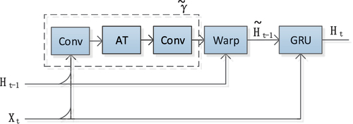
The TrajGRU unit was first established in Shi et al. (2017), which generates dynamic connection flow fields $U_t$ and $V_t$ by using a two-layer network γ. These flow fields are then utilized with bilinear sampling to sample $H_{\mathit{t}-1}$, as depicted in Figure 2. In this paper, axial attention is integrated into the TrajGRU network model’s sub-network, and the SA-TrajGRU unit with the self-attention mechanism is developed, as illustrated in Figure 3. The main formulas are given as follows:

Figure 2. The illustration of the TrajGRU unit. $X_t$ represents the input, $H_{\mathit{t}-1}$ represents the hidden state at time step t-1. γ denotes the sub-network within the TrajGRU model, which includes two convolutional recurrent neural networks (conv). Warp is the function used to select the dynamic connections. ${\tilde{H}}_{\mathit{t}-1}$ is the updated hidden state at time step t-1. GRU represents a GRU neural network model, and $H_t$ represents the hidden state at time step t.

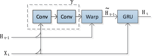
Figure 3. The illustration of the SA-TrajGRU unit. $X_t$ represents the input, and $H_{\mathit{t}-1}\mathit{\hspace{0.17em}}$represents the hidden state at time step t-1. At denotes the attention layer, and $\tilde{\gamma }$ represents the sub-network of the SA-TrajGRU unit, which includes two convolutional recurrent neural networks (conv) and the attention layer (AT). Warp is the function used to select the dynamic connections.$\mathit{\hspace{0.17em}}{\tilde{H}}_{\mathit{t}-1}$ represents the updated hidden state at time step t-1. GRU represents a GRU neural network model, and $H_t$ represents the hidden state at time step t.

$I_t=\mathrm{R}\mathit{elu}\left(W_{\mathit{xi}}\ast X_t+W_{\mathit{hi}}\ast H_{\mathit{t}-1}+b_i+b_h\right)$

$I_t=\mathit{A}{T}_h\left(I_t\right)+\mathit{A}{T}_v\left(I_t\right)$

$U_t,V_t=\underset{L}{\mathrm{split}}\left(W_{\mathit{ff}}\ast I_t+b_f\right)$

$Z_t=\mathit{\sigma }\left(W_{\mathit{xz}}\ast X_t+{\sum }_{l=1}^L{W}_{hz}^l\ast \mathit{warp}\left(H_{\mathit{t}-1},U_{\mathit{t},\mathit{l}},V_{\mathit{t},\mathit{l}}\right)\right)$

$R_t=\mathit{\sigma }\left(W_{\mathit{xr}}\ast X_t+{\sum }_{l=1}^L{W}_{hr}^l\ast \mathit{warp}\left(H_{\mathit{t}-1},U_{\mathit{t},\mathit{l}},V_{\mathit{t},\mathit{l}}\right)\right)$

$H_t^{\prime }=\tanh \left(W_{\mathit{xh}}\ast X_t+{R_t}^{\circ }\left({\sum }_{l=1}^L{W}_{hh}^l\ast \mathit{warp}\left(H_{\mathit{t}-1},U_{\mathit{t},\mathit{l}},V_{\mathit{t},\mathit{l}}\right)\right)\right)$

(1) $H_t={\left(1-Z_t\right)}^{\circ }{H}_t^{\prime }+{Z_t}^{\circ }{H}_{\mathit{t}-1}$(1)

Here, * denotes the convolution operation, and ° represents the Hadamard product. $\mathit{A}{T}_h$ is used to obtain the horizontal attention function, while $\mathit{A}{T}_v$ is to obtain the vertical attention function. L represents the total number of allowed links. The flow fields $U_t$ and $V_t$ store the dynamic connections generated by the network $\tilde{\gamma }$. The warp function selects the dynamic connections through bilinear sampling.

Under the sequence-to-sequence framework, we proposed a novel convolutional recurrent network named SA-TrajGRU, as shown in Figure 4. In the Encode part, the network architecture consists of three layers of convolution and SA-TrajGRU units, where the convolutional layers mainly perform downsampling to reduce the output image size and increase the number of channels. In the Decode part, the network architecture consists of three layers of deconvolution and SA-TrajGRU units, where the deconvolution layers primarily perform upsampling to increase the output image size. The parameter configurations for the SA-TrajGRU model are described in Table 1. For the convolution and deconvolution block, the Kernel column in the table represents the kernel size. For the SA-TrajGRU layers, the Kernel column represents the kernel size of input to state and state to state. Stride indicates the stride value for each layer, and CH I/O represents the input and output channel numbers for each corresponding layer.

Figure 4. Encode-decode architecture based on SA-TrajGRU units. $X_{\mathit{t}-1}$ and $X_t$ represent the input, while ${\tilde{X}}_{\mathit{t}+1}$ and ${\tilde{X}}_{\mathit{t}+2}$ represent the output. Conv refers to the convolution block, and SA-TrajGRU represents the SA-TrajGRU unit, and Deconv represents the deconvolution block.

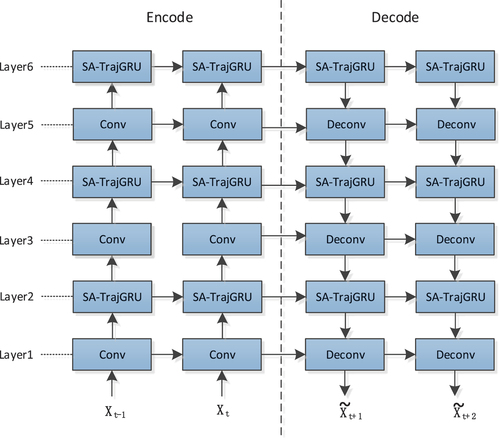
Table 1. The details of the SA-TrajGRU model.

Part	Layer	Kernel	Stride	Ch I/O	Type
Encode	Layer1	3×3	2	1/16	Conv
	Layer2	3×3	1	16/32	SA-TrajGRU
	Layer3	3×3	2	32/64	Conv
	Layer4	3×3	1	64/32	SA-TrajGRU
	Layer5	3×3	2	32/16	Conv
	Layer6	3×3	1	16/16	SA-TrajGRU
Decode	Layer6	3×3	1	16/16	SA-TrajGRU
	Layer5	3×3	2	16/32	Deconv
	Layer4	3×3	1	32/64	SA-TrajGRU
	Layer3	3×3	2	64/32	Deconv
	Layer2	3×3	1	32/16	SA-TrajGRU
	Layer1	3×3	2	16/1	Deconv

Experiments

To evaluate the performance of the model, synthetic image sequences from Moving MNIST-2 dataset and radar data from the CIKM AnalytiCup 2017 competition were used as the datasets. All experiments are implemented on the NVIDIA GeForce RTX 3080 Ti GPU platform using PyTorch. Each model is trained using the Adam optimizer (Kingma and Ba 2014) with an initial learning rate of 0.0004. Since the loss functions typically include L1 loss, L2 loss, and L1+L2 loss, we trained the reference models using L1, L2, and L1+L2 loss and found that they yield similar prediction results. Therefore, for the MovingMNIST and CIKM AnalytiCup 2017 datasets, we employ L2 Loss, i.e. Mean Squared Error (MSE) loss as the loss function. The MSE is calculated as follows:

(2) $\mathrm{MSE}=\frac{{\sum }_{n=1}^N{\sum }_{i=1}^h{\sum }_{j=1}^w{\left({\mathit{y}}_{\mathit{n},\mathit{i},\mathit{j}}-{\tilde{y}}_{\mathit{n},\mathit{i},\mathit{j}}\right)}^2}{\mathit{N}}$(2)

where N is the number of samples, h and w represent the height and width of the feature map, $y_{\mathit{n},\mathit{i},\mathit{j}}\mathit{\hspace{0.17em}}$ denotes the pixel value of the ground truth, and ${\tilde{y}}_{\mathit{n},\mathit{i},\mathit{j}}$ represents the pixel value of the prediction.

Experiment on moving MNIST-2

The Moving MNIST-2 experiment involves sampling two digits from the original MNIST dataset and generating synthetic image sequences by adjusting parameters such as rotation, direction, and speed. Each frame in the image sequence contains two handwritten digits, and the image size is 64 × 64 pixels. The synthetic image sequence dataset consists of 8,000 training samples, 2,000 validation samples, and 4,000 testing samples. The input consists of the first five frames of the image sequence, and the output consists of the subsequent 10 frames. In this experiment, the training process is stopped after 50, 000 iterations, and the mini-batch size is set to 16.

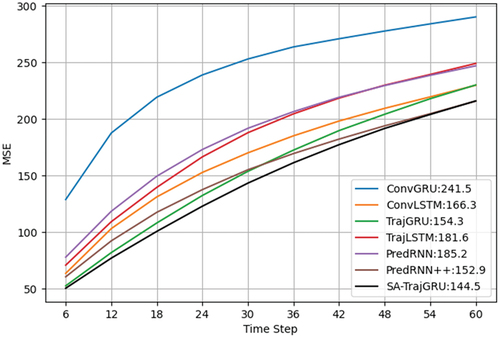
To present the performance of different models lead time, we present the frame-wise scores of the MSE on the Moving MNIST-2 test set in Figure 5. As shown in the figure, it is evident that the MSE value increases over time. We know that the MSE value reflects the prediction performance of the model, and a smaller MSE value indicates better performance. Therefore, all models show deteriorating prediction performance over time. Additionally, we can observe that our proposed SA-TrajGRU model, although exhibiting an increase in MSE value over time, consistently achieves the smallest MSE value compared to other models at the same time step. Consequently, the proposed SA-TrajGRU model consistently exhibits the best performance.

Figure 5. Frame-wise MSE comparisons of different models on the moving MNIST-2 test set. The numbers following the model names in the captions represent the average values of MSE.

Figure 6 shows the prediction case of different models on the Moving MNIST-2 test set. The first row represents the input sequence, the second row shows the ground truth, and the subsequent rows exhibit the predictions made by different models. We can compare the predicted images of different models with the ground truth images (the second row) to evaluate the model’s prediction performance. The closer the predicted images with the ground truth images, the better the prediction performance of the model. As depicted in Figure 6, we can see that as time increases, the prediction performance of all models become worse, and the predicted images become more and more blurry. From Figure 6, it can be observed that among all the models, the TrajGRU and SA-TrajGRU models can better preserve the details of the predicted images. Furthermore, upon careful observation of the predicted images of these two models, we can notice that the TrajGRU model exhibits some noise, whereas the proposed SA-TrajGRU model has less noise.

Figure 6. Prediction case on the moving MNIST-2 test set.

Experiment on radar data

The radar echo dataset used in this paper is from the CIKM AnalytiCup 2017 competition data. Specific data can be downloaded from the Tianchi Laboratory website on Alibaba Cloud, and the detailed download link in the Supplementary Materials. It covers an area of 101 km × 101 km in Shenzhen, with a horizontal resolution of 1 kilometer and a time resolution of 6 minutes. Each image in the dataset contains 101 × 101 pixels. The training dataset consists of 10,000 sequence samples, while the testing dataset contains 4,000 sequence samples. Each sequence sample contains 15 radar images. In the radar echo extrapolation experiment, we select the first five echo images from each sequence as the input, and the subsequent ten echo images as the predicted output. In other words, we use the radar echo data from the first 30 minutes to predict the radar echo data for the next 60 minutes.

In the experiment, all models were trained using pixel values. The training process is stopped after 80,000 iterations, and the mini-batch is set to 8, and pixel values of all the echo maps are normalized to a range of [−1.0 1.0]. The evaluation metrics for radar echo extrapolation include rainfall Root Mean Squared Error (Rainfall-RMSE), Heidke Skill Score (HSS), Critical Success Index (CSI), Probability of Detection (POD), and False Alarm Rate (FAR). The Rainfall-RMSE metric is defined as the average root mean squared error between the predicted rainfall and the ground truth. To calculate the predicted rainfall, first, we calculate the reflectivity dBZ by using the following formula (Luo, Li, and Ye 2020):

(3) $\mathrm{dBZ}=\mathrm{p}\ast 95/255-10$(3)

where p denotes pixel value. Then, we calculate the rainfall using the Z-R relationship: dBZ = 10 log a + 10b log R, where R is the rainfall rate in mm/h, and a, b are two constants with a = 200, b = 1.6. The calculated results are shown in Table 2. It can be seen that compared with those of ConvLSTM, TrajGRU,TrajLSTM, PredRNN, PredRNN++, and PFST-LSTM, the rainfall-RMSE of the SA-TrajGRU model is the smallest.

Table 2. Comparison of the average rainfall-RMSE scores of different models.

Precipitation intensity	Rainfall-RMSE(mm/h)
ConvGRU	35.574
ConvLSTM	5.346
TrajGRU	5.290
TrajLSTM	5.273
PredRNN	5.244
PredRNN++	5.170
PFST-LSTM	5.328
SA-TrajGRU	5.115

To calculate HSS, CSI, POD, FAR for a given reflectivity threshold τ, firstly, we convert the threshold τ to a pixel value p using the following formula:

(4) $\mathrm{p}=\left(\mathit{\tau }+10\right)\times 255/95$(4)

Then we compare the pixel value p against the predicted and ground truth values point to point. If p is greater than the predicted value, prediction = 1, otherwise, prediction = 0. Similarly, if p is greater than the ground truth value, truth = 1, otherwise, truth = 0. We can obtain TP (True Positive) when prediction = 1 and truth = 1, FP (False Positive) when prediction = 1 and truth = 0, TN (True Negative) when prediction = 0 and truth = 0, and FN (False Negative) when prediction = 0 and truth = 1. The calculation formulas for the evaluation metrics of HSS, CSI, POD, and FAR are as follows:

(5) $\mathrm{HSS}=\frac{\mathit{TP}\ast TN-FN\ast FP}{\left(\mathit{TP}+\mathit{FN}\right)\ast \left(\mathit{FN}+\mathit{TN}\right)+\left(\mathit{TP}+\mathit{FP}\mathit{\hspace{0.17em}}\right)\ast \left(\mathit{FP}+\mathit{TN}\right)}$(5)

(6) $\mathrm{CSI}=\frac{\mathit{TP}}{\mathit{TP}+\mathit{FP}+\mathit{FN}}$(6)

(7) $\mathrm{POD}=\frac{\mathit{TP}}{\mathit{TP}+\mathit{FN}}$(7)

(8) $\mathrm{FAR}=\frac{\mathit{FP}}{\mathit{TP}+\mathit{FP}}$(8)

HSS and CSI consider both the detection probability and the false alarm rate simultaneously, which can directly reflect the model’s performance. Hence, we choose HSS and CSI as evaluation metrics to assess the performance of radar echo extrapolation. We use the corresponding relationship between dBZ and precipitation (Zhang 2020), as shown in Table 3. We select 25, 35, and 45 dBZ as the thresholds to represent light rain, moderate rain, and heavy rain, and calculate HSS and CSI. Generally, a higher HSS and CSI indicate better model performance.

Table 3. Correspondence between dBZ and precipitation intensity.

Precipitation intensity	dBZ	Precipitation intensity (mm/h)
Light Rain	15–30	.2–2.0
Moderate Rain	30–40	2.0–10
Heavy Rain	40–45	10–30
Torrential Rain	46–50	30–50
Severe Rain	50–55	50–100
Extreme Rain	56–70	>100

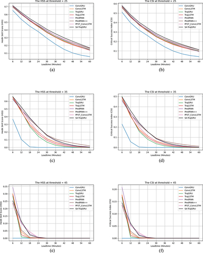
Figure 7 illustrates HSS and CSI scores of different models on the CIKM AnalytiCup 2017 test set under thresholds of 25, 35, and 45 dBZ. As shown in Figure 7, HSS and CSI scores of the model decrease over time under the same threshold. HSS and CSI scores of the SA-TrajGRU model are higher than scores of other models under the radar echo threshold of 25, indicating that the SA-TrajGRU model has the most accurate prediction results under this threshold. HSS and CSI scores of SA-TrajGRU are comparable to scores of PredRNN and PredRNN++ under the radar echo threshold of 35, indicating that the SA-TrajGRU, PredRNN and PredRNN ++ models have similar ability of prediction. HSS and CSI scores of PredRNN++, PFST_ConvLSTM, and SA-TrajGRU models are relatively higher than scores of other models under the radar echo threshold of 45.

Figure 7. HSS and CSI scores of different nowcast lead time. (a) HSS τ = 25 dBZ. (b) CSI τ = 25 dBZ. (c) HSS τ = 35 dBZ. (d) CSI τ = 35 dBZ. (e) HSS τ = 45 dBZ. (f) CSI τ = 45 dBZ.

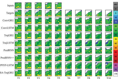
Figure 8 illustrates a prediction case of convective precipitation using different methods on the CIKM AnalytiCup 2017 test set. As can be seen, the prediction of all extrapolation methods become worse over time, and the predicted images become more and more blurred. In the whole stage, ConvGRU, ConvLSTM, TrajGRU and TrajLSTM model could only roughly predict the contours of the high-reflectivity areas, and the other models preserved more details in the radar echoes. From T1 to T6, we can see that the details of high-reflectivity areas of PredRNN, PredRNN++ and SA-TrajGRU models are well maintained, especially SA-TrajGRU model is more accurate in predicting location of high-reflectivity areas. From T7 to T10, compared with other models, SA-TrajGRU is better at predicting shape of the precipitating area. Similar phenomenon is also observed in other prediction cases.

Figure 8. Prediction case of convective precipitation on the CIKM AnalytiCup 2017 test set.

Conclusions

In this paper, we embed axial attention into the TrajGRU unit, and proposed a convolutional recurrent neural network with self-attention mechanism named SA-TrajGRU. Through experiments on the CIKM AnalytiCup 2017 radar echo dataset, we demonstrate that the performance of the proposed SA-TrajGRU model is comparable to other convolutional recurrent neural network models, and SA-TrajGRU model has the most accurate prediction results under the radar echo threshold of 25. However, the forecasting ability of this method degrades rapidly over time, especially in the high reflectivity region. In the future, the SA-TrajGRU model needs to be further optimized to improve the forecasting ability, especially in the high reflectivity region. Furthermore, to increase the usefulness of the study to the precipitation nowcasting audience, we will utilize Short-Term Ensemble Prediction System (STEPS) as a reference model for comparative analysis in our future work.

Acknowledgements

We acknowledge Pro. Xiangfeng Guan for providing English proofreading and valuable suggestion.

Data availability statement

The data that support the findings of this study are available the Tianchi Laboratory website on Alibaba Cloud. Data are available at https://tianchi.aliyun.com/dataset/1085 with the permission of Alibaba.

Disclosure statement

No potential conflict of interest was reported by the authors.

Supplementary material

Supplemental data for this article can be accessed online at https://doi.org/10.1080/08839514.2024.2311003.

Additional information

Funding

This work was supported by the Natural Science Foundation of Fujian Province of China (Nos.2021J011225, 2023J011099).

References

- Agrawal, S., L. Barrington, C. Bromberg, J. Burge, C. Gazen, and J. Hickey, 2019. Machine learning for precipitation nowcasting from radar images. Proceedings of the 33rd Conference on Neural Information Processing Systems, Vancouver, Canada,1–18. doi:10.48550/arXiv.1912.12132.
- Ayzel, G., M. Heistermann, and T. Winterrath. 2019. Optical flow models as an open benchmark for radar-based precipitation nowcasting (rainymotion v0.1). Geoscientific Model Development 12 (4):1387–1402. doi:10.5194/gmd-12-1387-2019.
- Ballas, N., L. Yao, C. Pal, and A. Courville. 2015. Delving deeper into convolutional networks for learning video representations. arXiv E-Prints. doi:10.48550/arXiv.1511.06432.
- Berenguer, M., D. Sempere-Torres, and G. G. S. Pegram. 2011. Sbmcast – an ensemble nowcasting technique to assess the uncertainty in rainfall forecasts by Lagrangian extrapolation. Canadian Journal of Fisheries and Aquatic Sciences 404 (3–4):226–40. doi:10.1016/j.jhydrol.2011.04.033.
- Bowler, N. E., C. E. Pierce, and A. W. Seed. 2004. Development of a rainfall nowcasting algorithm based on optical flow techniques. Canadian Journal of Fisheries and Aquatic Sciences 288 (1):74–91. doi:10.1016/j.jhydrol.2003.11.011.
- Bowler, N. E., C. E. Pierce, and A. W. Seed. 2006. STEPS: A probabilistic precipitation forecasting scheme which merges an extrapolation nowcast with downscaled NWP. Quarterly Journal of the Royal Meteorological Society 132 (620):2127–55. doi:10.1256/qj.04.100.
- Dixon, M., and G. Wiener. 1993. TITAN: Thunderstorm identification, tracking, analysis, and nowcasting—A radar-based methodology. Journal of Atmospheric and Oceanic Technology 10 (6):785. doi:10.1175/1520-0426(1993)010<0785:TTITAA>2.0.CO;2.
- Dosovitskiy, A., L. Beyer, A. Kolesnikov, D. Weissenborn, and N. Houlsby. 2020. An image is worth 16x16 words: Transformers for image recognition at scale. arXiv E-Prints. doi:10.48550/arXiv.2010.11929.
- Doviak, R. J., D. S. Zrnic, and R. M. Schotland. 1994. Doppler radar and weather observations. Applied Optics 33 (21):453.
- Ganguly, A. R., and R. L. Bras. 2002. Distributed quantitative precipitation forecasting using information from radar and numerical weather prediction models. Journal of Hydrometeorology 4 (6):1168–80. doi:10.1175/1525-7541(2003)004<1168:DQPFUI>2.0.CO;2.
- Guo, S. Z., D. Xiao, and X. Y. Yuan. 2017. Short-term rainfall prediction method based on neural network and model integration. Chinese Journal of Progress in Meteorological Science and Technology 7 (1):7.
- Handwerker, J. 2002. Cell tracking with TRACE3D—a new algorithm. Atmospheric Research 61 (1):15–34. doi:10.1016/S0169-8095(01)00100-4.
- Ho, J., N. Kalchbrenner, D. Weissenborn, and T. Salimans. 2019. Axial attention in multidimensional transformers. arXiv E-Prints. doi:10.48550/arXiv.1912.12180.
- Huang, Z., X. Wang, L. Huang, C. Huang, Y. Wei, and W. Liu. 2019. Ccnet: Criss-cross attention for semantic segmentation. In ICCV. doi:10.48550/arXiv.1811.11721.
- Johnson, J. T., P. L. Mackeen, A. Witt, E. D. W. Mitchell, G. J. Stumpf, M. D. Eilts, and K. W. Thomas. 1998. The storm cell identification and tracking algorithm: An enhanced WSR-88D algorithm. Weather and Forecasting 13 (2):263–76. doi:10.1175/1520-0434(1998)013<0263:TSCIAT>2.0.CO;2.
- Kingma, D., and J. Ba. 2014. Adam: A method for stochastic optimization. Computer science. arXiv E-Prints. doi:10.48550/arXiv.1412.6980.
- Klein, B., L. Wolf, and Y. Afek. 2015. A dynamic convolutional layer for short rangeweather prediction. Computer Vision & Pattern Recognition. IEEE. doi:10.1109/CVPR.2015.7299117.
- Lin, Z., M. Li, Z. Zheng, Y. Cheng, and C. Yuan. 2020. Self-attention ConvLSTM for spatiotemporal prediction. Proceedings of the AAAI Conference on Artificial Intelligence 34 (7):11531–38. doi:10.1609/aaai.v34i07.6819.
- Li, L., W. Schmid, and J. Joss. 1995. Nowcasting of motion and growth of precipitation with radar over a complex orography. Journal of Applied Meteorology 34 (6):1286–300. doi:10.1175/1520-0450(1995)034<1286:NOMAGO>2.0.CO;2.
- Luo, C., X. Li, Y. Wen, Y. Ye, and X. Zhang. 2021. A novel LSTM Model with interaction dual attention for radar echo extrapolation. Remote Sensing 13 (2):164. doi:10.3390/rs13020164.
- Luo, C., X. Li, and Y. Ye. 2020. PFST-LSTM: A SpatioTemporal LSTM Model with pseudoflow prediction for precipitation nowcasting. IEEE Journal of Selected Topics in Applied Earth Observations and Remote Sensing 99:1–1. doi:10.1109/JSTARS.2020.3040648.
- Mo, S., and N. Atanasov. 2017. A spatiotemporal model with visual attention for video classification. arXiv E-Prints. doi:10.48550/arXiv.1707.02069.
- Pulkkinen, S., D. Nerini, A. Pérez Hortal, C. Velasco-Forero, and L. Foresti. 2019. Pysteps – a community-driven open-source library for precipitation nowcasting. doi:10.13140/RG.2.2.31368.67840.
- Ranzato, M., A. Szlam, J. Bruna, M. Mathieu, R. Collobert, and S. Chopra. 2014. Video (language) modeling: a baseline for generative models of natural videos. arXiv E-Prints. doi:10.48550/arXiv.1412.6604.
- Rinehart, R. E., and E. T. Garvey. 1978. Three-dimensional storm motion detection by conventional weather radar. Nature 273 (5660):287–289. doi:10.1038/273287a0.
- Seed, A. W. 2003. A dynamic and spatial scaling approach to advection forecasting. Journal of Applied Meteorology 42 (3):381–88. doi:10.1175/1520-0450(2003)042<0381:ADASSA>2.0.CO;2.
- Shi, X., Z. Chen, H. Wang, D. Y. Yeung, W. K. Wong, and W. C. Woo. 2015. Convolutional LSTM network: A machine learning approach for precipitation nowcasting. arXiv e-prints. d oi: arXiv:1506.04214.
- Shi, X., Z. Gao, L. Lausen, H. Wang, D. Y. Yeung, W. K. Wong, and W.C. Woo. 2017. Deep learning for precipitation nowcasting: A benchmark and a new model. arXiv e-prints. doi:10.48550/arXiv.1706.03458.
- Shi, E., Q. Li, D. Q. Gu, and Z.M. Zhao. 2018. Radar echo extrapolation method based on convolutional neural network. Chinese Journal of Computer Applications 38 (3):6.
- Shi, H., Q. Zhou, Y. Ni, X. Wu, and L. J. Latecki. 2021. DPNET: Dual-path network for efficient object detectioj with lightweight self-attention. arXiv E-Prints. doi:10.48550/arXiv.2111.00500.
- Sønderby, C. K., L. Espeholt, J. Heek, M. Dehghani, A. Oliver, T. Salimans, S. Agrawal, J. Hickey, and N. Kalchbrenner. 2020. Metnet: A neural weather model for precipitation forecasting. arXiv E-Prints. doi:10.48550/arXiv.2003.12140.
- Srivastava, R. K., K. Greff, and J. Schmidhuber. 2015. Training very deep networks. Advances in Neural Information Processing Systems 2377–85. doi:10.48550/arXiv.1507.06228.
- Trebing, K., T. Staǹczyk, and S. Mehrkanoon. 2021. SmaAt-UNet: Precipitation nowcasting using a small attention-UNet architecture. Pattern Recognition Letters 145:178–186. doi:10.1016/j.patrec.2021.01.036.
- Tuttle, J. D., and G. B. Foote. 1990. Determination of the boundary layer airflow from a single doppler radar. Journal of Atmospheric and Oceanic Technology 7 (2):218–32. doi:10.1175/1520-0426(1990)007<0218:DOTBLA>2.0.CO;2.
- Wang, Y., Z. Gao, M. Long, J. Wang, and P. S. Yu. 2018. PredRNN++: Towards a resolution of the deep-in-time dilemma in spatiotemporal predictive learning. arXiv e-prints. doi:10.48550/arXiv.1804.06300.
- Wang, X., R. Girshick, A. Gupta, and K. He. 2018. Non-local neural networks. CVPR. doi:10.48550/arXiv.1711.07971.
- Wang, Y., M. Long, J. Wang, Z. Gao, and P. S. Yu. 2017. Predrnn: Recurrent neural networks for predictive learning using spatiotemporal lstms. 31st Conference on Neural Information Processing Systems (NIPS 2017), Long Beach, CA, USA, 879–888.
- Wang, Y., H. Wu, J. Zhang, Z. Gao, J. Wang, P. S. Yu, and M. Long. 2021. PredRNN: A recurrent neural network for spatiotemporal predictive learning. arXiv e-prints. doi:10.48550/arXiv.2103.09504.
- Wu, K., W. Liang, and S. Q. Wang. 2018. Regional rainfall forecast based on 3D convolutional neural network. Chinese Journal of Image and Signal Processing 7 (4):200–12. doi:10.12677/JISP.2018.74023.
- Wu, D., L. Wu, T. Zhang, W. Zhang, J. Huang, and X. Wang. 2022. Short-term rainfall prediction based on radar echo using an improved self-attention PredRNN deep learning model. Atmosphere 13 (12):1963. doi:10.3390/atmos13121963.
- Zhang, J. L. 2020. Research on method of precipitation prediction in severe convective weather based on deep learning. Nanjing University of Science and Technology.