Predication of Water Pollution Peak Concentrations by Hybrid BP Artificial Neural Network Coupled with Genetic Algorithm

ABSTRACT

Water pollutions can severely affect water environment, causing water quality degradation and threatening aquatic wildlife. Deemed as guideline for maximum environmental impact assessment, water pollution peak concentration (WPPC) has been intensively studied to organize effective countermeasures. In this study, a back propagation artificial neural network (BPANN) coupled with genetic algorithm (GA) was constructed to predict peak concentrations. Compared with BPANN, multiple linear regressions model (MLRM) and step-wise multiple linear regressions model (SMLRM), GA-BPANN model showed superior accuracy in both simulating and predicting peak concentrations (R² = 0.93 and 0.67 0.69 respectively). In 12 peak concentration cases, GA-BPANN model’s mean absolute relative error (MARE) ranges from 0.0 to 0.58, averaged at 0.09, significantly lower than BPANN, MLRM and SMLRM (MARE = 0.29, 0.45 and 0.48). Further analysis revealed that GA-BPANN model can be used as an effective and efficient tool for water quality simulation and early warning prediction.

Introduction

Water pollution refers to the increase of harmful substances in water bodies caused by human activities that reduce the quality of the water environment (Syeed et al. 2023). The main sources of pollution include industrial wastewater, urban and rural sewage, pesticides, fertilizers, heavy metals, etc. (Feng et al. 2024; Sun et al. 2023; Zhang et al. 2022a). Once pollutions occur, they will have serious impacts on the aquatic lives and pose potential health risk to those who use polluted waters as drinking sources. Toxic pollutants can even kill aquatic organisms directly, leading to a significant reduction or even extinction of aquatic populations, disrupting the food chain and biodiversity of the ecosystems. Besides, enduring water pollution poses severe threat to human health too. Drinking contaminated water can lead to health problems such as gastrointestinal diseases, liver diseases, or even cancers (Li et al. 2019a; Liu et al. 2022; Ugochukwu et al. 2022; Wiering, Kirschke, and Akif 2023; Zhou et al. 2022). Therefore, it is of great significance to predict the development of water pollution and peak concentration is often considered to be most vital information (Uddin, Nash, and Olbert 2021, 2022a,b 2023a). Since it usually serves as the basis for maximum environmental impact assessment (MEIA), and deemed as the guideline for effective countermeasures.

Predicting water pollution peaks is a complex problem that requires consideration of multiple natural and anthrogenic factors. To build a comprehensive mathematical model usually involves basic sub-processes, such as weather conditions, hydrodynamics, bio-chemical processes, ecological cycles, social production, and emission (Abouelsaad et al. 2022; Alasl et al. 2012; Ambrose, Wool, and Barnwell 2009; Burchard-Levine et al. 2014). There are now many effective and efficient ways to construct such models, among which numerical models based on pollutant transportive and reactive processes, and data-driven models based on linear or non-linear projective functions are most wildly used and well recognized (Ding et al. 2023; Duraisamy, Iaccarino, and Xiao 2019; Georgescu et al. 2023; Hao et al. 2021; Markus et al. 2010). Numerical models, in most cases, are built on rigorous physical, chemical, or biological fundamentals, which on one hand can simulate and represent spatial and temporal water quality variations objectively (Costa et al. 2021; Li et al. 2021; Yu et al. 2022), while on the other hand, inevitably necessitate geographic, hydrologic, meteorological and water quality survey abundance, which might not be so easy to collect, especially when study cases are located in remote or under-developed areas. Data-driven models are those that fully recognize, analyze, and utilize multivariate data through various data-mining and info-reconstructive technologies like machine learning and artificial intelligence (Pany, Rath, and Swain 2023; Uddin et al. 2023a,c; Wang et al. 2021). For instance, by introducing machine learning algorithms to reconfigure water quality index models, the modified WQI models are proved to be more objective, data-driven, and less susceptible to eclipsing and ambiguity errors (Uddin et al. 2023d,e). Artificial Neural Network (ANN), as an AI-based technique to solve various nonlinear problems, also becomes more and more popular in different fields, due to the its capabilities in nonlinear projection, self-learning, and adaptation (Kim, Cho, and Recknagel 2023; Kumar et al. 2024).

The study area, Wujiang, is a typical sub-tropic river in southern China. It originates in the remote mountains of Hunan province and flows into Guangdong, where it eventually confluents with Beijiang which serves as drinking water source for millions of local residents and millions more for the downstream Pearl River Delta (PRD). For years, Wujiang has been constantly bothered by mining and metal smelting enterprises in upper Hunan province. Cross-border lead pollutions induced by storm overflow and factory accidental spills put a high risk to the region and become the center of public scrutiny. Lead, especially dissolved absorbable Lead, is one kind of heavy metal that can jeopardize human digestive, immune or nerve systems, causing nausea, loss of appetite, vomiting, bloating or diarrhea, etc. if reaching acute high level (Abbaszade et al. 2022). Although local government has built state-of-art water quality auto-monitoring stations at the provincial border of Wujiang, to monitor heavy metal variations, the corelative relationship between cross border water quality and downstream drinking water source is still not clear. Impact assessment and prediction of inbound water quality conditions on downstream drinking water sources remain a huge challenge to the local government.

The objective of this paper is to develop an improved BPANN model to predict dissolved lead concentrations (DLC) at downstream stations, based on the data obtained at upstream border. GA (Genetic Algorithm) is used to make up for the defects of BPANN model by incorporating multi-dimensional parallel optimization functions. Major efforts of this paper include:

1. To implement hybrid GA-BPANN and other models on DLC peak concentration simulation and prediction in a typical remote mountain river of southern China.

2. To evaluate model performance of GA-BPANN, BPANN and multiple linear regression models in terms of peak concentration precision comparison.

3. To assess capabilities of various models to reflect nonlinearity and time-delay phenomenon of pollution concentration variation.

The work here provides guidance for decision-making and early warning purposes on lead pollution control, maximum environmental impact assessment and potential ecological and health risk evaluation.

Materials and Methods

Study Area

Wujiang originates from Chenzhou city, Hunan Province, and flows southeast into Guangdong Province. Chenzhou is renowned as “world nonferrous metals museum,” where more than 110 types of minerals, valued exceeding RMB 260 billion, have been discovered (Liao et al. 2005; Yuan and Chen 2018; Zhou et al. 2022). Among those minerals, lead and zinc ores are the main and most popular resources in the market. Owing to the rich natural metal mineral resources, a large number of metal mining, smelting and metal manufacturing plants have gathered locally. Years of industrial production have discharged large amounts of heavy metal-rich wastewater and residues into the environment, resulting in serious pollution of water and soil in local areas (Ding et al. 2017; Xu et al. 2015). In recent years, although the local government has invested large number of resources to control heavy metal pollution, strictly requiring polluting enterprises to achieve standard emissions, and point source pollution has been effectively managed and controlled, local upstream tributary sediments, tailings mines, and soil pollution remains severe, requiring longer periods of treatment and restoration. Whenever a heavy rainfall event occurs, the release of sediment from tributaries and a large amount of non-point source heavy metal pollution can directly lead to serious pollution of heavy metals in the main stream of the Wujiang River, threatening the water quality safety of downstream water sources in Guangdong (Li et al. 2019a; Li et al. 2019b; Wu and Chen 2010).

Sampling and QA/QC Measures

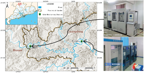
Since 2013, Guangdong Province has built a high-precision water quality automatic monitoring station (WQAMS), Sanxi station, at the Wujiang provincial border of Hunan and Guangdong to monitor the physical, chemical, and heavy metal indicators. A similar WQAMS, Pingshi station, was built at downstream local drinking water source to ensure that Wujiang water quality is safe for drinking standards. The distance between the two WQAMS is approximately 40 kilometers, with two major tributaries- Nanhua river and Yizhang river, converging from south and north bank respectively (Figure 1).

Figure 1. Sampling stations of Sanxi and Pinshi WQAMS along Wujiang river.

Both WQAMS take water samples at 4 hours interval daily. To ensure the data quality, auto-monitoring equipment is checked manually on site and apparatus precision is calibrated by standard samples every week. Manual sampling comparison experiments between automatic monitoring and indoor laboratory are carried out monthly, to ensure that WQAMS’ results are in accordance with conventional manual monitor data. Every year, a thorough maintenance procedure on apparatus accuracy, precision, detection limit, and other related parameters is tested, verified, updated, or repaired if damaged. Last but not the least, daily data are strictly audited online and anomalies will be checked and handled by local maintenance crew or by sending online commands by control center to trigger off one of the six different types of remote QA/QC procedures shown in Figure 2.

Figure 2. Sanxi WQAMS online simulator and monitor panel.

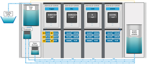
①Blank sample calibration, ② Standard sample calibration, ③ Low level standard sample check, ④ High level standard sample check, ⑤ Standard solution check, ⑥ Duplicate sample analysis.

Data Description

The water quality monitoring indicators include water temperature, pH, conductivity (Cond), dissolved oxygen (DO), turbidity (Turb), ammonia nitrogen, total phosphorus (TP), total nitrogen (TN), copper, lead, zinc, arsenic, etc. The meteorological indicators used are the daily rainfall and water elevation from the Sanxi Station published by the Guangdong Provincial Water Resources Department (http://210.76.80.76:9001/#/rainfall). Based on Pearson correlation analysis, five indicators of Pb, water level, rainfall, pH, and turbidity in the Sanxi Water Station were initially selected as input variables for the model to predict the concentration of Pb in the downstream Pingshi Water Station.

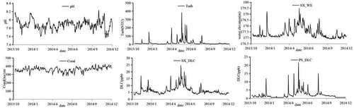
446 days of Data from Oct. 11^th, 2013 to Dec. 31^th, 2014 was collected. Each indicator was daily averaged in the first place, to eliminate possible data noise interference. By ticking off invalid data induced by instrumental malfunctions, system maintenance and QA/QC procedures, 430 days of paired dataset were put in use for this research (Figure 3). Upstream water quality and hydrodynamic indicators including pH, Cond, Turb, DLC and water elevation data from Sanxi WQAMS were used as input to predict downstream DLC level at Pingshi WQAMS.

Figure 3. Sampling stations of Sanxi and Pinshi WQAMS along Wujiang river.

Model Development

The proposed hybrid model is developed from BPANN, which is known for its unique capability to fit any non-linear function or process at any precision. However, its single point searching scheme for optimal structural parameters can easily fall into trap for local but global optimal results, which ultimately undermines the accuracy and reliability of the model. In this case, the introduction of GA, known for its parallel optimization capability, is necessary to avoid that defect. To demonstrate the efficiency and accuracy of the GA-BPANN, model performance comparisons were conducted with BPANN model and two other linear models, MLRM and SMLRM.

BPANN

BP ANN models are originated from recent knowledge of signal transition and interactions between brain and its associated nervous systems and often used to approximate functions that have no definite formations or data series about which we have little knowledge at all. BPANN is one of the most widely used neural network models. Its characteristic is that it adopts the process separation operation mode of forward propulsion of simulation and prediction and backward propagation of error correction. According to the direction of error reduction between the predicted output value and the actual value, the connection weights and thresholds between nodes and neurons are corrected layer by layer to ensure the continuous improvement of network simulation and prediction accuracy.

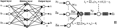
A basic 3-layer interconnected neural network as Figure 4, comprised of an input layer, a hidden layer and an output layer, is often found to be competent to fit and predict complex environmental processes. The input layer consists of one or more input nodes, each of which are connected to the adjacent hidden layer nodes known as “Neurons.” Neurons are also connected in the same way to the output layer nodes.

Figure 4. Illustrative map of a typical 3-layer BPANN.

The construction process of BPANN usually includes three stages: input data initialization, network training and simulation/prediction.

(1) Input data initialization. The main purpose of initialization is to eliminate the gradient difference between data sequences caused by dimensional difference among multiple input variables. Transformation of the input variables into standardized values between 0 and 1 is wildly formulated as follows:

$\widetilde{x_i}=\frac{x_i-x_{\mathit{min}}}{x_{\mathit{max}}-x_{\mathit{min}}}$

In which，x_i,x_max and x_min represent the ith, maximum and minimum input values.

(2) Network training. The network training process is mainly to fit the connection weights and thresholds between the input layer and the middle layer, and between the middle layer and the output layer. Each neuron node in the middle layer S_i defines as.

$S_i={\sum }_{p=1}^m(w_{\mathit{pi}}\times x_p)-{\theta }_i$

$L_j={\sum }_{i=1}^n(v_{\mathit{ij}}\times \mathit{f}(S_i))-{\gamma }_j$

Neuron node further transmits the accumulated input information to the output layer node through the transfer function f(x) as:

$\mathit{f}\left(\mathit{x}\right)=\frac{1}{1-{\mathit{e}}^{-\mathit{x}}}$

The prediction error E is calculated as follows, and used to readjust the weights and thresholds of each layer in reverse direction.

$\mathit{E}=\sum _{\mathit{i}=1}^N\sum _{\mathit{j}=1}^k{\left({\mathit{y}}_{\mathit{ij}}-{\hat{y}}_{\mathit{ij}}\right)}^2$

$\left\{\begin{array}{c}{{\mathit{v}}_{\mathit{ij}}}^{\mathit{l}+1}={{\mathit{v}}_{\mathit{ij}}}^{\mathit{l}}-\mathit{\lambda }\frac{\mathrm{\partial E}}{{{\mathit{v}}_{\mathit{ij}}}^{\mathit{l}}}\\ {{\gamma }_j}^{\mathit{l}+1}={{\gamma }_j}^{\mathit{l}}-\mathit{\lambda }\frac{\mathrm{\partial E}}{{{\gamma }_j}^{\mathit{l}}}\\ {{\mathit{w}}_{\mathit{pi}}}^{\mathit{l}+1}={{\mathit{w}}_{\mathit{pi}}}^{\mathit{l}}-\mathit{\lambda }\frac{\mathrm{\partial E}}{{{\mathit{w}}_{\mathit{pi}}}^{\mathit{l}}}\\ {{\theta }_i}^{\mathit{l}+1}={{\theta }_i}^{\mathit{l}}-\mathit{\lambda }\frac{\mathrm{\partial E}}{{{\theta }_i}^{\mathit{l}}}\end{array}\right.$

(3) Simulation/prediction. After the weight and threshold are corrected, the error E value is recalculated. If it is less than the preset minimum value, it means that the model converges to the desired level, then the training is finished; otherwise, the iteration will continue until the accuracy requirements are met or the maximum training times are reached.

GA-BPANN

The basic idea of the hybrid genetic neural network model is to use the powerful multidimensional parallel optimization of genetic algorithm to make up for the defects of the traditional artificial neural network model based on the weight and threshold correction method by the reverse error gradient, to avoid the “optimal illusion” of the local extremum in the process of parameter optimization of ANN model (Muttil et al. 2005; Mulia et al. 2013).

GA is an optimization method of parallel random search developed based on natural biological genetics and evolution theory. By introducing the concepts of gene, chromosome, population, and fitness function, and using data coding and decoding, population individual selection, chromosome cross replication, gene mutation and other operations, the complex and cumbersome parameter optimization process is transformed into the biological evolution and evolution process of “survival of the fittest,” which can effectively avoid the optimization result falling into the local optimal value rather than the global optimum. Moreover, GA also has distinctive advantages in self-organizing, adapting, and self-learning capabilities. Obtaining information from genetic evolutionary process of self-organized optimal search, GA allows only the individuals with higher fitness function value or higher probability of survival to evolve into upgraded genetic structures so that continuous improvements can be assured.

The basic GA subprocesses include:

1. Coding process. It is the process of converting commonly used decimal data into binary or real string code, so that it can be used for subsequent corresponding evolutionary algorithms.

2. Decoding process. It is the reverse of the encoding process, which restores the encoded data to decimal data.

3. Selection. The selection operation is to select some individuals in the old population with a certain probability, and then inherit and evolve them into the new population. The individual selection probability is related to the fitness function value. The higher the fitness, the greater the selection probability.

4. Crossover. The crossover operation is to generate new excellent individuals through the exchange and combination of single or multipoint positions of two individual chromosomes, and then complete the individual evolution process.

5. Mutation. The mutation process is the process of mutation operation on any position gene in random individuals, so as to produce new excellent individuals.

The coupling strategy is to use GA to search for the optimal neural structure and function weights and coefficients (Yi et al. 2022). The general procedures are as follows,

1. Create a basic structure of a BP-ANN, including layers of the network, nodes in each layer, and stimulus function formations etc., mostly based on the input and output sample data characteristics.

2. Randomly generalize a set of weights and thresholds coefficients for BP-ANN, which are the main object of GA optimization. Initialize GA primary parameters, including generation numbers, population size, crossover and mutation probability. Generation numbers control the number of times genes evolve and can be served as the termination condition for the entire algorithm.

3. Set up population size, which equals the number of chromosome individuals in each generation and intimately affects the convergence speed and efficiency of GA.

4. Set up crossover probability, which controls the frequency of use of the crossover operator, which can accelerate convergence and reach the most promising optimal solutions. Therefore, a larger crossover probability is generally chosen, but too high a crossover probability may also lead to premature convergence.

5. Set up mutation probability, which controls the frequency of use of mutation operators and determines the local search ability of genetic algorithms, these parameters are generally preliminarily determined based on the scale and range of the data to be processed, and multiple experiments are required to obtain parameters with better application effects.

6. Represent the objective function of optimization with fitness values; iterates selection, crossover, and mutation procedures, aiming to downsize convergence error between BP-ANN output values and observed records. Once fitness value reaches pre-set thresholds or evolution times exceeds generation number, the GA optimization process will be terminated.

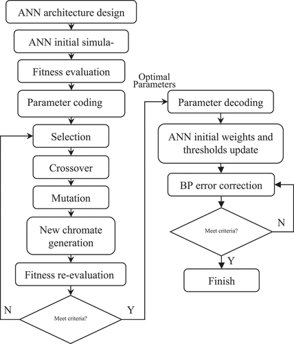
A simplified schematic flowchart is demonstrated as follows in Figure 5:

Figure 5. Schematic flowchart of hybrid GA-BPANN.

MLRM

MLRM is a way of multiple linear regressions and often refers to a linear regression model with multiple explanatory variables, which is used to explain the linear relationship between the explained variable and other multiple explanatory variables (Rossi et al. 2022). Its basic format is as follows:

$\mathit{y}=\mathit{\epsilon }+{\beta }_0+{\beta }_1{x}_1+{\beta }_2{x}_2+\cdots +{\beta }_m{x}_m$

Where β₀ is the constant term, also known as the intercept. β₁, β₂, …, β_m is named as partial regression coefficient or simply regression coefficient. The equation indicates that the response variable y in the data can be approximated as a linear function of the independent variables x₁, x₂, …, x_m. ε is the random error (i.e., residual) after removing the effects of the m independent variables on y. The partial regression coefficient β_j (j = 1, 2, …, m) represents the average change in y when x_j is changed by one unit while the other independent variables are held constant.

The model parameters β₁, β₂, …, β_m are estimated from the sample data to obtain the multiple linear regression equation:

$\hat{y}=b_0+b_1{x}_1+b_2{x}_2+\cdots +b_m{x}_m$

Where b₀, b₁, b₂, …, b_m are the estimates of the model parameters and $\hat{y}$ is the estimated value of y, which represents the mean value of y when a set of independent variables x₁, x₂, …, x_m are taken.

As with simple linear regression, the parameter estimates for the multiple linear regression model can be obtained by the least squares method, i.e., minimizing the sum of squares of the residuals based on the observed n cases of data:

$\mathrm{Q}={\sum }_{k=1}^n{\left(y_k-{\hat{y}}_{\mathit{k}}\right)}^2={\sum }_{k=1}^n{\left[y_k-\left(b_0+b_1{x}_{1\mathit{k}}+b_2{x}_{2\mathit{k}}+\cdots +b_m{x}_{\mathit{mk}}\right)\right]}^2$

Mathematically, b₀, b₁, b₂, …, b_m can be obtained by solving the system of equations and finding the constant term b₀ of the regression equation by the following equation:

$\{\begin{array}{c}{l}_{11}{b}_1+l_{12}{b}_2+\dots +l_{1\mathit{m}}{b}_m=l_{1\mathit{y}}\\ \dots \dots \\ l_{\mathit{m}1}{b}_1+l_{\mathit{m}2}{b}_2+\dots +l_{\mathit{mm}}{b}_m=l_{\mathit{my}}\end{array}$

$l_{\mathit{ij}}=\sum \left(x_i-{\bar{x}}_{\mathit{i}}\right)\left(x_j-{\bar{x}}_{\mathit{j}}\right)=\sum x_i{x}_j-\frac{\sum x_i\sum x_j}{\mathit{n}}$

$l_{\mathit{iy}}=\sum \left(x_j-{\bar{x}}_{\mathit{j}}\right)\left(\mathrm{y}-{\bar{y}}_{\mathit{j}}\right)=\sum x_j\mathit{y}-\frac{\sum x_j\sum \text{nolimitsy}}{\mathit{n}}$

$\mathit{i},\mathit{j}=1,2,\dots ,\mathit{m}$

$b_0=\bar{y}-\left(b_1{\bar{x}}_1+b_2{\bar{x}}_2+\cdots +b_m{\bar{x}}_{\mathit{m}}\right)$

where l_ij is the sum of the off-mean-squared differences of the independent variables (i=j) or the sum of the off-mean products of the two independent variables (i≠j). l_iy is the sum of the off-mean products of the independent variable x_j and the response variable y.

SMLRM

Stepwise multiple linear regressions model (SMLRM) is a way of multiple linear regressions (Radovanović et al. 2022; Sharma et al. 2015; Zounemat-Kermani et al. 2014). After each new independent variable is introduced forward, the previously selected independent variables are reexamined to evaluate their value of remaining in the equation. For this purpose, the introduction and elimination are alternated until there are no new statistically significant variables to be introduced and no statistically significant variables to be eliminated.

Only one independent variable is introduced or excluded at each step. Whether an independent variable is introduced or excluded depends on the F-test or the corrected coefficient of determination of its partial regression sum of squares (Wiegand et al. 2010).

If (m‒1) independent variables have been introduced in the equation, and the variable x_j is introduced on top of it, the regression sum of squares of the equation (i.e., containing m independent variables) after the introduction of x_j is SS₁ and the residual is SS₂. The regression sum of squares of the previous equation containing (m-1) independent variables (excluding x_j) is SS₃, the partial regression sum of squares of x_j is U = SS₁–SS₃. The test statistic can be expressed by the following equation:

$F_j=\frac{U}{S{S}_2/\left(\mathit{n}-\mathit{m}-1\right)}$ (F_j follows Fα (1, n – m − 1) distribution)

In which, U is the partial regression sum of squares of x_j, (i.e., U = SS₁–SS₃). Generally, the value of α is taken as 0.05.

If F_j > Fα(1, n − m − 1), then x_j is selected into the equation. Otherwise, it is not selected. The process is reversed by removing the statistically insignificant independent variables from the equation, but the test is the same.

Model Performance Evaluation

To evaluate accuracy and effectiveness of various models, Mean Absolute Relative Error (MARE) and coefficient of determination (R²) is used as follows (Georgescu et al. 2023; Uddin et al. 2023c,f,g):

$\mathit{MARE}=\frac{1}{N}\sum _{\mathit{i}=1}^N\frac{\left(\widehat{y_i}-y_i\right)}{y_i}\times 100\mathrm{\%}$

$R^2=1-\frac{1}{N}\frac{{\sum }_1^N{\left(\widehat{y_i}-y_i\right)}^2}{{\sum }_1^N{\left(y_i-\hat{y}\right)}^2}$

In which, $\widehat{y_i}$, $\hat{y}$ , y_i are modeled, mean modeled and observed value.

Moreover, Pearson coefficients are used to evaluate datasets correlation and consistency by SPSS22.0 software.

Results and Discussion

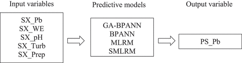
In order to predict DLC concentration variation at Pingshi (represented by PS_Pb), a group of variables, major information of upstream Sanxi town, including DLC (SX_Pb), water elevation(SX_WE), precipitation (SX_prep) and water chemical species like pH (SX_Ph), conductivity (SX_Cond) and turbidity (SX_Turb), was incorporated and used as input variables for GA-BPANN, BPANN, MLRM and SMLRM models, as shown in Figure 6.

Figure 6. Model input and output structure.

Descriptive Statistics of Input/Output Data

Data from October 2013 to July 2014 are used as the basis for model construction and calibration; Data from August 2014 to December 2014 are the model verification materials. Descriptive statistics of calibration data (as in Table 1) and predictive data (as in Table 2) show that mean value and standard deviation of DLC at Pingshi are lower than in Sanxi, which means that water quality level and variation at the provincial border are higher and more volatile. The skewness and kurtosis coefficients also reveal that Sanxi’s DLC process is more leptokurtic distributed than Pingshi. Skewness of SX_pH and SX_Cond are less than 1.645, which can be interpreted as that these indices are more normalized distributed than other indices. Kurtosis of SX_Prep, SX_Turb and SX_Pb are the highest, indicating that these indices have the most radical transition process and are potentially interactive.

Table 1. Descriptive statistics of calibration data from Oct. 2013 to July 2014.

Species	N	Min.	Max.	Mean	Std.	Skewness	Kurtosis
PS_Pb	304	0.50	21.51	2.15	2.40	3.78	20.2
SX_Pb	289	3.11	24.54	7.01	3.22	1.96	5.31
SX_WE	296	177	179.5	177	0.46	1.54	2.19
SX_Prep	304	0	71.5	3.24	8.76	4.37	23.8
SX_ pH	289	7.6	8.18	7.89	0.11	0.14	0.20
SX_Cond	289	281	412	355	24.9	−0.42	0.13
SX_Turb	289	2.00	383	21.9	38.9	5.15	34.2

Table 2. Descriptive statistics of predictive data from Aug. 2014 to Dec. 2014.

Species	N	Min.	Max.	Mean	Std.	Skewness	Kurtosis
PS_Pb	152	0.50	15.0	1.56	1.47	5.67	47.9
SX_Pb	152	3.25	11.6	5.03	1.18	2.07	8.81
SX_WE	152	177	179	177	0.28	2.12	5.93
SX_Prep	153	0	52.0	2.83	8.33	3.92	16.4
SX_ pH	153	7.57	8.24	7.87	0.13	−0.15	−0.04
SX_Cond	153	287	429	375	24.2	−0.55	0.93
SX_Turb	153	4.00	108	9.38	11.1	6.76	52.6

Model Application and Evaluation

General Evaluation

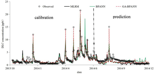
BPANN, GA-BPANN, MLRM and SMLRM were implemented to simulate and predict DLC process at Pingshi station. GA-BPANN turns out to be most accurate in both calibration and prediction phase, especially at the peak concentration simulation. Meanwhile, BPANN is more precise than MLRM and SMLRM, as shown in Figure 7.

Figure 7. Calibration and prediction of DLC at Pinshi station by MLRM, BPANN and GA-BPANN.

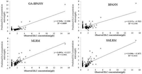
Linear correlative analysis between observed and simulated DLC of Pingshi station during calibration phase was conducted to evaluate accuracy of various models.GA-BPANN has the highest R² value at 0.9284, far exceeds R² value by BPANN, MLRM and SMRM at 0.7993,0.7087 and 0.7, as shown in Figure 8.

Figure 8. Linear corelative analysis between observed and simulated DLC of Pingshi station at calibration phase.

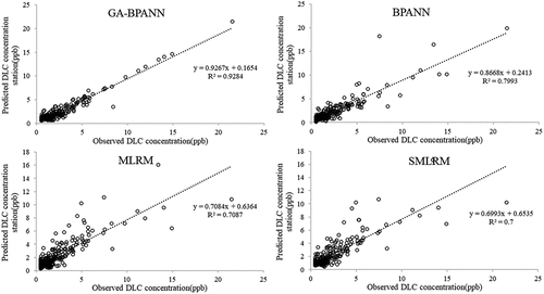
GA-BPANN also has the highest R² value at 0.6699, far exceeds R² value by BPANN, MLRM and SMRM at 0.3794,0.5943 and 0.4533, as shown in Figure 9. In general, GA-BPANN prevails in both calibration and prediction phases and turns out to be the more efficient than BPANN in reaching an error convergence.

Figure 9. Linear corelative analysis between observed and simulated DLC of Pingshi station at predictive phase.

Peak Concentration Evaluation

12 major peak concentrations were selected for comparison as shown in Table 3. It turns out that GA-BPANN generates the best calibrated and predictive results, AREs range between 0.0% to 57.8%, averaged at 9.0%. 9 cases ARE is lower than 5%, 11 cases ARE is lower than 20%. BP-ANN shows lower accuracy compared with GA-BPANN, ARE range between 8% to 59% and averaged at 29%. Meanwhile none is below 5%, with only 2 cases lower than 10%. Linear regression models like MLRM and SMLRM are comparatively much less accurate than GA-BPANN and BP-ANN. Peak concentration predication errors are generally over 20%, range between 17% to 163% and 19% to 118% respectively. and average AREs are 45% and 48%. R² comparison reveals that GA-BPANN is highest in both calibration and verification phases, BP ANN has higher R² than MLRM and SMLRA in calibration phase, but lower in verification phase (Table 3).

Table 3. Simulated DLC(SDLC) and ARE by various models.

Date	DLC (ppb)	Modeled DLC (ppb)				MARE (%)
		MLRM	SMLRA	BPANN	GA-BPANN	MLRM	SMLRA	BPANN	GA-BPANN
2013/11/13	2.15	5.65	4.68	3.31	1.85	163%	118%	54%	14%
2013/12/17	11.97	7.97	8.19	11.04	11.95	33%	32%	8%	0%
2014/3/13	2.77	4.27	4.25	3.53	2.66	54%	54%	28%	4%
2014/4/1	14.03	9.58	9.40	10.19	14.03	32%	33%	27%	0%
2014/4/27	14.90	6.41	6.94	10.19	14.66	57%	53%	32%	2%
2014/5/13	5.53	4.48	4.45	3.88	4.52	19%	20%	30%	18%
2014/5/19	21.51	10.85	10.18	19.87	21.49	50%	53%	8%	0%
2014/5/23	11.17	9.02	9.07	9.50	11.10	19%	19%	15%	1%
2014/6/4	7.54	6.23	5.83	6.32	7.34	17%	23%	16%	3%
2014/6/11	9.77	7.15	7.28	5.69	9.78	27%	25%	42%	0%
2014/7/2	8.39	3.27	3.24	3.43	3.54	61%	61%	59%	58%
2014/8/20*	15.04	7.19	7.28	8.40	14.34	52%	52%	44%	5%
Min.	2.15	3.27	3.24	3.31	1.85	17%	19%	8%	0%
Max.	21.51	10.85	10.18	19.87	21.49	163%	118%	59%	58%
Average	10.40	6.84	6.73	7.95	9.77	48%	45%	29%	9%
R^2 in calibration phase	-					0.71	0.70	0.80	0.93
R^2 in verification phase						0.59	0.45	0.38	0.67

ppb means part per billion, is the unit of concentrations

Discussion

The mechanism of non-point source pollution caused by rainfall runoff is very complex, involving multiple natural factors such as hydrology, meteorology, ecology, and environment. The peak impact factors that form river pollution clusters are more complex, and the relationship is also more complex. Existing research suggests that when significant rainfall occurs, it generally first forms surface runoff on the ground surface. DLC in the soil enters the water body under the erosion and leaching of rainwater or surface runoff, and then flows into the river, forming varying degrees of peak processes in hydrodynamic processes such as advection and diffusion in the river. Among them, rainfall intensity, rainfall duration, spatial distribution of rainfall, land use status of the basin, Soil type, DLC content in soil and its dissolution property, surface slope, distance between polluted land and river, natural slope of the river, sediment content, pH, flow rate and flow rate are all important factors affecting the peak concentration (Lin et al. 2024; Qiao et al. 2023; Su et. al. 2022; Yu et al. 2023; Zou et al. 2024). And these factors play different roles in different rainfall intensities, different levels of Soil contamination and different types of rivers. At present, there are also some water quality pollution models based on the mechanism of rainfall runoff, such as the SWAT model recommended by the US EPA, HSPF model, etc. However, their structure is very complex, and the requirements for basic data are extremely strict. Moreover, the model has hundreds of internal parameters, and the calibration and validation process are very complicated and time consuming, which is very unfavorable for areas lacking data.

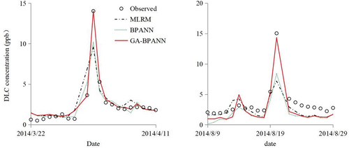
The coupling relationship between the factors that affect the peak concentration of water pollutions is complex and usually nonlinear. First, pollution sources, especially non-point sources, are often volatile. Its distribution, duration and intensity are highly corelated to rain precipitation (Lei et al. 2023; Poudyal, Cochrane, and Bello-Mendoza 2021), land use and slope (Agbeshie and Abugre 2021; Badalge et al. 2024; Zhang et al. 2022a, b), soil property (Ding et al. 2017), vegetation (Li et al. 2024; Tan et al. 2024) etc. Secondly, water quality’s response to source loading variations is nonlinear due to the non-linear physical advection and dispersion processes of water environment. besides, biochemical degradation of pollutants is also not linear, especially when environmental factors like water temperature, turbidity, or solar radiation etc. changes (Su et al. 2022; Sun et al. 2024). Figure 10 provides two predictive cases by ANNs and linear models. GA-BPANN stands out and achieves the best predictive precision on April 1^st and August 20^th peaks.

Figure 10. Typical peak DLC process simulation by various models.

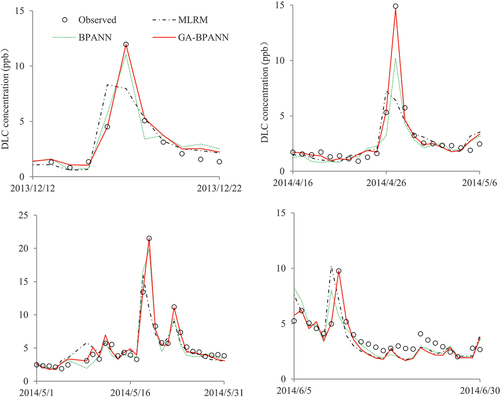
Other studies have also shown that in addition to the nonlinear superposition effect of multiple factors of non-point source pollution on peak concentration, it can also lead to significant time delay effects in some specific cases (Cuss et al. 2021; Schmidt et al. 2021; Xie et al. 2024). From the perspective of mechanism analysis, if there is spatial consistency between the rainfall concentration area and the heavily polluted land area, the peak concentration of pollution is generally synchronized with the peak flow of the river. If inconsistent, it is generally later than the peak transportation. Since general linear model equations do not consider the time delay effect of multiple factors on peak concentration processes, it is very difficult or even impossible to predict the delayed process. This article found in four typical peak concentration cases that MLRM cannot simulate the prediction of peaks with time-delay properties. However, in comparison, the GA-BPANN model can effectively solve the time-delay prediction problem in all cases and achieve the highest prediction accuracy as shown in Figure 11.

Figure 11. Typical peak DLC process simulation by various models.

In general, the fitting accuracy error of linear models, including MLRM and SMLRM models, is more than 40%. GA-BPANN model prevails in every peak concentration prediction, with an averaged Absolute relative error of 9% (Table 3). The cause of differentiated performance, we believe, owes to the model structure and the nature of the peak pollution process. As a highly nonlinear problem as discussed above, peak pollution process is, in most cases, a nonlinear coupling of numbers of nonlinear relevant processes, such as hydrodynamics, biochemical cycling, and meteorological forcings etc. Typical linear regression models like MLRM and SMLRM, project predictions by linear combination of independent factors (Borode and Olubambi 2023; Selim et al. 2023; Sterc et al. 2023). So, if coupling relationship among these factors is linear, it can achieve accurate predictions, otherwise it may fail. BP network, on the other hand, uses an input-output pattern mapping scheme to represent mathematical equations or process. The stimulus functions it employs, equipped with weights variables to add up, and thresholds values to control the impulse of data information from each node, play an important role in approximation of a target function or process. Its backpropagation error adjustment algorithm ensures that the sum of square errors of the network will keep in a descending direction, and further enhances its ability to fit linear or nonlinear predictions (García-Alba et al. 2019; Haggerty et al. 2023).

Conclusion

A hybrid BPANN model enhanced by GA is proposed and applied to peak concentration prediction and could be used in early warning purposes for future water pollution incidents. The introduction of parallel searching scheme of GA to BPANN helps to achieve better performance in both calibrate and predictive simulations. From this research study, the following conclusions can be drawn:

• GA-BPANN outperformed original BPANN, and MLRM/SMLRM linear regression models in cases of peak concentration prediction. GA-BPANN had the lowest MARE (9%) and highest R² (0.93 and 0.67 at calibrate and predictive phase), followed by BP ANN, which was resulted in a slightly higher MARE (29%) and lower R² (0.80and 0.38).

• Compared with linear regression models, ANNs may get better MARE results, but BPANN’s predictive R² (0.38) is relatively lower, indicating that conventional ANN needs reinforced modification for further improvement.

• Peak pollution concentration simulations revealed that GA-BPANN could result in higher accuracy and superior capability in fitting coupling nonlinear pollution processes, and could also solve the problems of time delay phenomena.

• In general, GA-BPANN demonstrated acceptable precision in simulating water pollution peaks in both timing and concentration predictions, and could be used as an effective tool for future water quality early-warning.

Despite of the improvement of GA-BPANN, we found that there are potential challenges and problems that need to be addressed in future applications. Especially, in extreme case scenarios, when pollutant concentration is exceedingly low, GA-BPANN seems to less effective and performs poorer than linear regression models, suggesting that it may need to incorporate certain pattern recognition algorithm and set proper thresholds to filter or adjust predictive outputs.

Disclosure Statement

No potential conflict of interest was reported by the author(s).

Additional information

Funding

The work was supported by Major Science and Technology Program for Water Pollution Control and Treatment [2014ZX07206-005-003-001] funded by Ministry of Science and Technologyof the People’s Republic of China.; R&D projects in key areas of Guangdong Province [2020B1111350001].

References

- Abbaszade, G., D. Tserendorj, N. Salazar-Yanez, D. Zacháry, P. Völgyesi, E. Tóth, and C. Szabó. 2022. Lead and stable lead isotopes as tracers of soil pollution and human health risk assessment in former industrial cities of Hungary. Applied geochemistry 145:105397. doi:10.1016/j.apgeochem.2022.105397.
- Abouelsaad, O., E. Matta, M. Omar, and R. Hinkelmann. 2022. Numerical simulation of dissolved oxygen as a water quality indicator in artificial lagoons–case study el gouna. Egypt Regional Studies in Marine Science 56:102697. doi:10.1016/j.rsma.2022.102697.
- Agbeshie, A. A., and S. Abugre. 2021. Soil properties and tree growth performance along a slope of a reclaimed land in the rain forest agroecological zone of Ghana. Scientific African 13:e00951. doi:10.1016/j.sciaf.2021.e00951.
- Alasl, M. K., M. Khosravi, M. Hosseini, G. R. Pazuki, and R. Nezakati Esmail Zadeh. 2012. Measurement and mathematical modelling of nutrient level and water quality parameters. Water Science & Technology 66 (9):1962–24. doi:10.2166/wst.2012.333.
- Ambrose, R. B., T. A. Wool, and T. O. Barnwell. 2009. Development of water quality modeling in the United States. Environmental Engineering Research 14 (4):200–10. doi:10.4491/eer.2009.14.4.200.
- Badalge, N. D. K., J. Kim, S. Y. Lee, B. J. Lee, and J. Hur. 2024. Land use effects on spatiotemporal variations of dissolved organic matter fluorescence and water quality parameters in watersheds, and their interrelationships. Journal of Hydrology 631:130840. doi:10.1016/j.jhydrol.2024.130840.
- Borode, A., and P. Olubambi. 2023. Modelling the effects of mixing ratio and temperature on the thermal conductivity of GNP-Alumina hybrid nanofluids: A comparison of ANN, RSM, and linear regression methods. Heliyon 9 (8):e19228. doi:10.1016/j.heliyon.2023.e19228.
- Burchard-Levine, A., S. Liu, F. Vince, M. Li, and A. Ostfeld. 2014. A hybrid evolutionary data driven model for river water quality early warning. Journal of Environmental Management 143:8–16. doi:10.1016/j.jenvman.2014.04.017.
- Costa, C. M. D. S. B., I. R. Leite, A. K. Almeida, and I. K. de Almeida. 2021. Choosing an appropriate water quality model–A review. Environmental Monitoring and Assessment 193 (1):1–15. doi:10.1007/s10661-020-08786-1.
- Cuss, C. W., M. Ghotbizadeh, I. Grant-Weaver, M. B. Javed, T. Noernberg, and W. Shotyk. 2021. Delayed mixing of iron-laden tributaries in large boreal rivers: Implications for iron transport, water quality and monitoring. Journal of Hydrology 597:125747. doi:10.1016/j.jhydrol.2020.125747.
- Ding, Q., G. Cheng, Y. Wang, and D. Zhuang. 2017. Effects of natural factors on the spatial distribution of heavy metals in soils surrounding mining regions. Science of Total Environment 578:577–85. doi:10.1016/j.scitotenv.2016.11.001.
- Ding, F., W. J. Zhang, S. H. Cao, S. L. Hao, L. Y. Chen, X. Xie, W. P. Li, and J. M. Jiang. 2023. Optimization of water quality index models using machine learning approaches. Water Research 243:120337. doi:10.1016/j.watres.2023.120337.
- Duraisamy, K., G. Iaccarino, and H. Xiao. 2019. Turbulence modeling in the age of data. Annual Review of Fluid Mechanics 51 (1):357–77. doi:10.1146/annurev-fluid-010518-040547.
- Feng, H. Y., J. Schyns, S. Maarten, M. Kroll, M. J. Yang, H. Su, Y. Y. Liu, Y. P. Lv, X. B. Zhang, K. Yang, et al. 2024. Water pollution scenarios and response options for China. Science of the Total Environment 914:169807–13. doi:10.1016/j.scitotenv.2023.169807.
- García-Alba, J., J. F. Barcena, C. Ugarteburu, and A. García. 2019. Artificial neural networks as emulators of process-based models to analyse bathing water quality in estuaries. Water Research 150:283–95. doi:10.1016/j.watres.2018.11.063.
- Georgescu, P. L., S. Moldovanu, C. Iticescu, M. Calmuc, V. Calmuc, C. Topa, and L. Moraru. 2023. Assessing and forecasting water quality in the Danube River by using neural network approaches. Science of the Total Environment 879:162998–14. doi:10.1016/j.scitotenv.2023.162998.
- Haggerty, R. J. X. S., H. F. Yu, Y. S. Li, and Y. Li. 2023. Application of machine learning in groundwater quality modeling – a comprehensive review. Water Research 233:119745. doi:10.1016/j.watres.2023.119745.
- Hao, J., Y. Lin, G. Ren, G. Yang, X. Han, X. Wang, and Y. Feng. 2021. Comprehensive benefit evaluation of conservation tillage based on BP neural network in the Loess Plateau. Soil and Tillage Research 205:104784. doi:10.1016/j.still.2020.104784.
- Kim, H. G., K. H. Cho, and F. Recknagel. 2023. Time-series modelling of harmful cyanobacteria blooms by convolutional neural networks and wavelet generated time-frequency images of environmental driving variables. Water Research 246:120662. doi:10.1016/j.watres.2023.120662.
- Kumar, M. A., N. Srinivas, P. Ramya, N. Ahlawat, J. Sharma, and F. Vinod. 2024. Monitoring the quality of ground water in pipelines using deep neural network model. Groundwater for Sustainable Development 24:101073. doi:10.1016/j.gsd.2023.101073.
- Lei, K. G., Y. Li, Y. B. Zhang, S. Y. Wang, E. Yu, F. Li, F. Xiao, and F. Xia. 2023. Development of a new method framework to estimate the nonlinear and interaction relationship between environmental factors and soil heavy metals. Science of the Total Environment 905:167133. doi:10.1016/j.scitotenv.2023.167133.
- Liao, X., T. Chen, H. Xie, and Y. Liu. 2005. Soil as contamination and its risk assessment in areas near the industrial districts of Chenzhou City, Southern China. Environment international 31 (6):791–98. doi:10.1016/j.envint.2005.05.030.
- Li, T., Y. Liu, S. Lin, Y. Liu, and Y. Xie. 2019b. Soil pollution management in China: A brief introduction. Sustainability 11 (3):556. doi:10.3390/su11030556.
- Lin, F., H. L. Ren, J. S. Qin, M. Q. Wang, M. Shi, Y. C. Li, R. J. Wang, and Y. M. Hu. 2024. Analysis of pollutant dispersion patterns in rivers under different rainfall based on an integrated water-land model. Journal of Environmental Management 354:120314. doi:10.1016/j.jenvman.2024.120314.
- Li, R., C. Y. Tang, X. Li, T. Jiang, Y. P. Shi, and Y. J. Cao. 2019a. Reconstructing the historical pollution levels and ecological risks over the past sixty years in sediments of the Beijiang River, South China. Science of the Total Environment 649:448–60. doi:10.1016/j.scitotenv.2018.08.283.
- Liu, Z. Y., Y. Fei, H. D. Shi, L. Mo, and J. X. Qi. 2022. Prediction of high-risk areas of soil heavy metal pollution with multiple factors on a large scale in industrial agglomeration areas. Science of the Total Environment 808:151874–12. doi:10.1016/j.scitotenv.2021.151874.
- Li, D., Y. Wei, Z. Dong, C. Wang, and C. Wang. 2021. Quantitative study on the early warning indexes of conventional sudden water pollution in a plain river network. Journal of Cleaner Production 303:127067. doi:10.1016/j.jclepro.2021.127067.
- Li, J. X., L. C. Wu, L. M. Chen, J. Zhang, Z. H. Shi, J. X. Li, L. C. Wu, L. M. Chen, J. Zhang, Z. H. Shi, et al. 2024. Effects of slopes, rainfall intensity and grass cover on runoff loss of mercury from floodplain soil in Oak Ridge TN: A laboratory pilot study. Geoderma 441:116750. doi:10.1016/j.geoderma.2023.116750.
- Markus, M., M. I. Hejazi, P. Bajcsy, O. Giustolisi, and D. A. Savic. 2010. Prediction of weekly nitrate-N fluctuations in a small agricultural watershed in Illinois. Journal of Hydroin-Formatics 12 (3):251–61. doi:10.2166/hydro.2010.064.
- Mulia, I. E., H. Tay, K. Roopsekhar, and P. Tkalich. 2013. Hybrid ANN–GA model for predict-ing turbidity and chlorophyll-a concentrations. Journal of Hydro-Environment Research 7 (4):279–99. doi:10.1016/j.jher.2013.04.003.
- Muttil, N., and J. H. Lee. 2005. Genetic programming for analysis and real-time prediction of coastal algal blooms. Ecological Modelling 189 (3–4):363–76. doi:10.1016/j.ecolmodel.2005.03.018.
- Pany, R., A. Rath, and P. C. Swain. 2023. Water quality assessment for River Mahanadi of Odisha, India using statistical techniques and artificial neural networks. Journal of Cleaner Production 417:137713. doi:10.1016/j.jclepro.2023.137713.
- Poudyal, S., T. A. Cochrane, and R. Bello-Mendoza. 2021. Carpark pollutant yields from first flush stormwater runoff. Environmental Challenges 5:100301. doi:10.1016/j.envc.2021.100301.
- Qiao, P. W., S. Wang, J. B. Li, Q. Y. Zhao, Y. Wei, M. Lei, J. Yang, and Z. G. Zhang. 2023. Process, influencing factors, and simulation of the lateral transport of heavy metals in surface runoff in a mining area driven by rainfall: A review. Science of the Total Environment 857:159119. doi:10.1016/j.scitotenv.2022.159119.
- Radovanović, S., M. Milivojević, B. Stojanović, S. Obradović, D. Divac, and N. Milivojević. 2022. Modeling of Water Losses in Hydraulic Tunnels under Pressure Based on Stepwise Regression Method. Applied Sciences 12(18):9019. doi: 10.3390/app12189019.
- Rossi, E., I. Pecorini, and R. Iannelli. 2022. Multilinear regression model for biogas production prediction from dry anaerobic digestion of OFMSW. Sustainability 14 (8):4393. doi:10.3390/su14084393.
- Schmidt, S. I., J. Hejzlar, J. KopᡠCek, M. C. Paule-Mercado, P. Porcal, and Y. Vystavna. 2021. Relationships between a catchment-scale forest disturbance index, time delays, and chemical properties of surface water. Ecological Indicators 125:107558. doi:10.1016/j.ecolind.2021.107558.
- Selim, A., S. N. A. Shuvo, M. M. Islam, M. Moniruzzaman, S. Shah, and M. Ohiduzzaman. 2023. Predictive models for dissolved oxygen in an urban lake by regression analysis and artificial neural network. Total Environment Research Themes 7 (7):100066. doi:10.1016/j.totert.2023.100066.
- Sharma, M. J., and S. J. Yu. 2015. Stepwise regression data envelopment analysis for variable reduction. Applied Mathematics and Computation 253:126–34. doi:10.1016/j.amc.2014.12.050.
- Sterc, T. B., B. Filipovic-Grcic, B. Fran, and K. Mesic. 2023. Methods for estimation of OHL conductor temperature based on ANN and regression analysis. International Journal of Electrical Power & Energy Systems 151:109192. doi:10.1016/j.ijepes.2023.109192.
- Sun, H., X. Y. Hu, X. H. Yang, H. Wang, and J. H. Cheng. 2023. Estimating water pollution and economic cost embodied in the mining industry: An interprovincial analysis in China. Resources Policy 86:104284–12. doi:10.1016/j.resourpol.2023.104284.
- Sun, Y. X., Q. S. Jiang, R. Zou, W. J. Ma, M. C. Hu, Y. H. Chen, and Y. Liu. 2024. Exploring nonlinear responses of lake nutrients and algal blooms to restoration measures: A three-dimensional flux network modelling approach. Journal of Hydrology 631:130723. doi:10.1016/j.jhydrol.2024.130723.
- Su, H., R. Zou, X. L. Zhang, Z. Y. Liang, R. Ye, and Y. Liu. 2022. Exploring the type and strength of nonlinearity in water quality responses to nutrient loading reduction in shallow eutrophic water bodies: Insights from many numerical simulations. Journal of Environmental Management 313:115000. doi:10.1016/j.jenvman.2022.115000.
- Syeed, M., M. Hossain, M. Karim, F. Uddin, M. Hasan, and R. Khan. 2023. Surface water quality profiling using the water quality index, pollution index and statistical methods: A critical review. Environmental and Sustainability Indicators 18 (3):100247–23. doi:10.1016/j.indic.2023.100247.
- Tan, X. Y., Y. W. Jia, D. W. Yang, C. W. Niu, and C. Hao. 2024. Impact ways and their contributions to vegetation-induced runoff changes in the loess plateau. Journal of Hydrology: Regional Studies.51:101630. doi:10.1016/j.ejrh.2023.101630.
- Uddin, M. G., M. T. M. Diganta, A. M. Sajib, A. Rahman, S. Nash, T. Dabrowski, R. Ahmadian, M. Hartnett, and A. I. Olbert. 2023. Assessing the impact of COVID-19 lockdown on surface water quality in Ireland using advanced Irish water quality index (IEWQI) model. Environmental Pollution 336:122456. doi:10.1016/j.envpol.2023.
- Uddin, M. G., S. Nash, and A. Olbert. 2021. A review of water quality index models and their use for assessing surface water quality. Ecological Indicators 122:107218–21. doi:10.1016/j.ecolind.2020.107218.
- Uddin, M. G., S. Nash, A. Rahman, and A. Olbert. 2022a. A comprehensive method for improvement of water quality index (WQI). Water Research 219:118532. doi:10.1016/j.watres.2022.118532.
- Uddin, M. G., S. Nash, A. Rahman, and A. Olbert. 2022b. A comprehensive method for improvement of water quality index (WQI) models for coastal water quality assessment. Water Research 216:118532–20. doi:10.1016/j.watres.2022.118532.
- Uddin, M. G., S. Nash, A. Rahman, and A. Olbert. 2023a. Assessing optimization techniques for improving water quality model. Journal of Cleaner Production 385:135671. doi:10.1016/j.jclepro.2022.135671.
- Uddin, M. G., S. Nash, A. Rahman, and A. Olbert. 2023b. Marine waters assessment using improved water quality model incorporating machine learning approaches. Journal of Environmental Management 344:118368. doi:10.1016/j.jenvman.2023.118368.
- Uddin, M. G., S. Nash, A. Rahman, and A. Olbert. 2023c. A novel approach for estimating and predicting uncertainty in water quality index model using machine learning approaches. Water Research 229:119422–21. doi:10.1016/j.watres.2022.119422.
- Uddin, M. G., S. Nash, A. Rahman, and A. Olbert. 2023d. Performance analysis of the water quality index model for predicting water state using machine learning techniques. Process Safety and Environmental Protection 169:808–28. doi:10.1016/j.psep.2022.11.073.
- Uddin, M. G., S. Nash, A. Rahman, and A. Olbert. 2023e. A sophisticated model for rating water quality. Science of the Total Environment 868:161614. doi:10.1016/j.scitotenv.2023.161614.
- Uddin, M. G., A. Rahman, S. Nash, M. T. M. Diganta, A. M. Sajib, M. Moniruzzaman, and A. Olbert. 2023. Comparison between the WFD approaches and newly developed water quality model for monitoring transitional and coastal water quality in Northern Ireland. Science of the Total Environment 901:165960. doi:10.1016/j.scitotenv.2023.165960.
- Ugochukwu, U. C., N. Chukwuone, C. Jidere, B. Ezeudu, C. Ikpo, and J. Ozor. 2022. Heavy metal contamination of soil, sediment, and water due to galena mining in Ebonyi State Nigeria: Economic costs of pollution based on exposure health risks. Journal of Environmental Management 321:115864–69. doi:10.1016/j.jenvman.2022.115864.
- Wang, J., Y. Geng, Q. Zhao, Y. Zhang, Y. Miao, X. Yuan, W. Zhang, and W. Zhang. 2021. Water quality prediction of water sources based on meteorological factors using the CA-NARX approach. Journal of Environmental Modeling & Assessment 26 (4):529–41. doi:10.1007/s10666-021-09759-5.
- Wiegand, R. E. 2010. Performance of using multiple stepwise algorithms for variable selection. Statistics in Medicine 29 (15):1647–59. doi:10.1002/sim.3943.
- Wiering, M., S. Kirschke, and N. U. Akif. 2023. Addressing diffuse water pollution from agriculture: Do governance structures matter for the nature of measures taken? Journal of Environmental Management 332:117329–9. doi:10.1016/j.jenvman.2023.117329.
- Wu, B., and T. B. Chen. 2010. Changes in hair arsenic concentration in a population exposed to heavy pollution: Follow-up investigation in Chenzhou City, Hunan Province, Southern China. Journal of Environmental Sciences 22 (2):283–89. doi:10.1016/S1001-0742(09)60106-6.
- Xie, D. N., B. Zhao, R. H. Kang, X. X. Ma, T. Larssen, Z. D. Jin, and L. Duan. 2024. Delayed recovery of surface water chemistry from acidification in subtropical forest region of China. Science of the Total Environment 912:169126. doi:10.1016/j.scitotenv.2023.169126.
- Xu, B., Q. Xu, C. Liang, L. Li, and L. Jiang. 2015. Occurrence and health risk assessment of trace heavy metals via groundwater in Shizhuyuan Polymetallic Mine in Chenzhou City, China. Front Environmental Science and Engineering 9 (3):482–93. doi:10.1007/s11783-014-0675-8.
- Yi, X., Z. Wang, S. Liu, X. Hou, and Q. Tang. 2022. An accelerated degradation durability evaluation model for the turbine impeller of a turbine based on a genetic algorithms back-propagation neural network. Applied Sciences 12 (18):9302. doi:10.3390/app12189302.
- Yuan, S., and J. Chen. 2018. Analysis on the construction of nonferrous metal logistics park in ZX City of Hunan Province. In 2018 International Conference on Economy, Management and Entrepreneurship (ICOEME 2018). Atlantis Press, 224–27. doi:10.1016/j.gexplo.2014.09.010
- Yu, H., G. Jin, S. Jin, Z. Chen, W. Fan, and D. Xiao. 2022. Numerical modeling of COD transportation in Liaodong Bay: Impact of COD loads from rivers flowing into the sea. Water 14 (19):3114. doi:10.3390/w14193114.
- Yu, Q. W., Z. H. Sun, J. Y. Shen, X. Xu, Q. Y. Han, and M. Zhu. 2023. The nonlinear effect of new urbanization on water pollutant emissions: Empirical analysis based on the panel threshold model. Journal of Environmental Management 345:118564. doi:10.1016/j.jenvman.2023.118564.
- Zhang, Y., S. J. Granger, M. A. Semenov, H. R. Upadhayay, and A. L. Collins. 2022a. Diffuse water pollution during recent extreme wet-weather in the UK Environmental damage costs and insight into the future. Journal of Cleaner Production 338:130633–12. doi:10.1016/j.jclepro.2022.130633.
- Zhang, Z. Y., J. L. Huang, J. Bian, Y. Huang, J. Cai, and J. Bian. 2022b. Use of interpretable machine learning to identify the factors influencing the nonlinear linkage between land use and river water quality in the Chesapeake Bay watershed. Ecological Indicators 140:108977. doi:10.1016/j.ecolind.2022.108977.
- Zhou, L. F., X. L. Zhao, Y. B. Meng, Y. Yang, M. M. Teng, F. H. Song, and F. C. Wu. 2022. Identification priority source of soil heavy metals pollution based on source-specific ecological and human health risk analysis in a typical smelting and mining region of South China. Ecotoxicology & Environmental Safety 242:113864–11. doi:10.1016/j.ecoenv.2022.113864.
- Zou, Y. W., S. Lou, Z. R. Zhang, S. G. Liu, X. S. Zhou, F. Zhou, L. D. Radnaeva, E. Nikitina, and I. V. Fedorova. 2024. Predictions of heavy metal concentrations by physiochemical water quality parameters in coastal areas of Yangtze river estuary. Marine Pollution Bulletin 199:115951. doi:10.1016/j.marpolbul.2023.115951.
- Zounemat-Kermani, M., and M. Scholz. 2014. Modeling of dissolved oxygen applying stepwise regression and a template-based fuzzy logic system. Journal of Environmental Engineer-Ing 140 (1):69–76. doi:10.1061/(ASCE)EE.1943-7870.0000780.