Precision in Insurance Forecasting: Enhancing Potential with Ensemble and Combination Models based on the Adaptive Neuro-Fuzzy Inference System in the Egyptian Insurance Industry

ABSTRACT

Enhancing the precision of retention ratio predictions holds profound significance for insurance industry decision-makers and those vested in advancing insurance services. Precision helps insurance companies navigate inflationary pressures and evaluate underwriting profitability, enabling reliable prognoses of future underwriting gains. As far as we know, although there have been multiple attempts to construct a predictive model for retention ratio, none of these attempts have used combining models or studied the Egyptian market. Therefore, this study contributes significantly to this developing field by providing combining models, which combined statistical time series models such as Exponential Smoothing (ES), and Autoregressive Integrated Moving Average (ARIMA), with Adaptive Neuro-Fuzzy Inference System (ANFIS). Two different types of combinations are employed with these models. Furthermore, the study introduces three ensemble models designed for the purpose of predicting the retention ratio within the Egyptian insurance market. Dataset was carefully gathered from the EFSA’s annual reports, focused on the property-liability insurance sector within the Egyptian insurance market and covers the time period from 1989 to 2021. Next, the proposed models are assessed employing well-established statistical assessment metrics, namely, Mean Absolute Error (MAE), Mean Absolute Percent Error (MAPE), R Square (R²), and Root Mean Square Error (RMSE). The results show that combining and ensemble methods improve predicted accuracy. A multi-linear regression-based ensemble model that combines ARIMA, ES, and ANFIS models outperforms both single and combined models in robustness. The article concludes that the insurance industry can greatly benefit from modern predictive methods to make sound decisions.

Introduction

The insurance industry is a critical component of any economy, as insurance companies contribute significantly to the stability of the financial system. In recent times, the industry has undergone rapid changes, and intense competitive pressures have forced insurance firms to adopt competitive strategies that improve their financial performance.

One key metric that is widely used by insurance companies to evaluate their performance is the premium retention ratio. This ratio enables insurers to assess their profitability, risk management strategies, competitive positioning, and financial stability, while also providing a measure of the efficiency of key functions such as underwriting, reinsurance, and claims compromise. Forecasting, which represents a vital tool for predicting the future and planning strategies, is also essential from an economic standpoint (Cappiello 2020; Lee and Lee 2012).

The retention ratio significantly contributes to insurance businesses achieving their objectives. The retention ratio is a crucial indicator used to evaluate the effectiveness of underwriting decisions and the industry’s potential for success. It indicates the percentage of risks that insurance companies choose not to transfer to reinsurance. Companies with higher retention ratios tend to have better underwriting methods and are more inclined to generate positive results (Hasibuan, Sadalia, and Muda 2020). Research in the overall insurance sector focuses on choosing appropriate statistical techniques to get precise estimations of the correlation between variables. To ensure the validity of the analysis and testing, these estimates need to be precise, effective, and uniform.

Forecasting is a vital technique that enables insurance businesses to anticipate future results and formulate strategies accordingly. Thus, accurate and efficient forecasting systems are highly sought after in this industry. To this end, modern predictive methods are increasingly being employed by insurance companies to obtain accurate predictions of the premium retention ratio. This enables them to make sound decisions and build resilience against financial challenges and economic downturns (Khalil, Liu, and Ali 2022). Consequently, techniques for accurate and effective forecasting are in high demand, and insurance companies seek to employ modern predictive methods to obtain accurate predictions for the premium retention ratio. These predictions aid companies in making sound decisions and enhance their ability to face financial challenges and economic downturns (Hasibuan, Sadalia, and Muda 2020).

Several methods of predicting have been proposed across various areas. Nevertheless, traditional statistical methods for analyzing time series data, such in (Adnan et al. 2017; Box et al. 2015; Hu et al. 2013; Karia, Bujang, and Ahmad 2013; Khashei and Bijari 2011; Lai et al. 2006; Soliman Osama 2003; Taha, Ibrahim, and Minai 2011; Zhang et al. 2017), and these techniques are classified into two categories Time series models such as the exponential smoothing model (ES), and the autoregressive integrated moving average model (ARIMA) are powerful forecasting tools used in many applications (Asadollahfardi et al. 2018), and complex prediction issues have been resolved with the aid of causal models like regression models, which employ the theory of cause and effect and the identification of influential components (Majid and Ahmad Mir 2018). However, these techniques have some drawbacks on generalization issue, satisfy the statistical assumptions, and treating with subjectivity, uncertainty, and small data, that can extent in issue of insurance industry. In addition, for sequences with random and nonlinear properties, it was challenging to mine the information accurately and effectively using statistical models (Fu et al. 2021). On the other hand, the efficacy of Artificial Intelligence (AI) techniques, such as the Adaptive Neuro-Fuzzy Inference System (ANFIS), has been widely studied in various application areas, and historical and recent research indicate that ANFIS can outperform conventional forecasting methods. ANFIS, a hybrid machine learning model, combines the strengths of both Artificial Neural Networks (ANNs) and Fuzzy Logic Systems (FLSs), thereby offering the advantages of both methods (Chen et al. 2018; Namal; Rathnayake, Dang, and Hoshino 2021).

In recent years, the integration of combining and ensemble methods into predictive models has significantly advanced the accuracy and reliability of predictions. These methods have the potential to enhance decision-making in various industries, including finance and economics, by providing valuable insights into the underlying patterns in the data. Therefore, it is essential to continue exploring and developing these approaches to improve the accuracy and robustness of predictive models (Bokaba, Doorsamy, and Sena Paul 2022; Liu et al. 2020; Matloob et al. 2021). The benefits of these approaches have been well documented in the literature, as they provide a more comprehensive and holistic perspective when modeling complex systems. Moreover, they are capable of handling high-dimensional data with varying degrees of complexity and noise, which makes them particularly useful in practical applications. Consequently, there has been a significant research effort in developing new and innovative combining and ensemble methods, as well as refining existing ones, to improve their performance and applicability across different domains. The field of predictive modeling is constantly evolving, and combining and ensemble methods are expected to play a crucial role in advancing this field in the years to come (Bokaba, Doorsamy, and Sena Paul 2022).

Despite these considerable efforts, there are still a dearth of review studies that evaluate the forecasting models used in the performance ratios forecasting of insurance companies and discuss the models from a more multivariate standpoint. To address this gap, this research offers significant contributions to the field of prediction methods and insurance company performance. The study’s primary objective is to improve predictability and develop an accurate model for regulators to predict performance and rank insurance companies. To achieve this goal, this study introduces predictive frameworks utilizing both ARIMA-ANFIS and ES-ANFIS methodologies. Additionally, the study proposes various ensemble models which utilize ARIMA, ES, and ANFIS models based on multi-linear regression to predict the retention ratio of the Egyptian insurance market. The primary intent of these models is to enhance the precision in predicting the retention ratio within the Egyptian insurance market. Such models not only furnish insightful projections for retention ratios but also help actuaries in their professional responsibility of making strategic choices in the insurance companies and offer significant practical implications for the insurance sector. The research presents several significant contributions to the insurance literature as outlined below:

1. The authors suggest a variety of combination and ensemble predictive models to enhance the accuracy of retention ratio predictions for Egyptian insurance firms. The combination models integrate statistical models with the ANFIS in various manners, depending on either the error of the statistical models or their predicted outcomes. The ensemble models employ a stacking methodology, amalgamating the inputs of ARIMA, EXP, and ANFIS grounded on multi-linear regression models. Four metrics are proposed to evaluate the prediction performance in all models. These methodologies given can overcome the limitations of solely using individual models and effectively manage challenges in insurance data, such as uncertainty and limited dataset size and assist actuaries in fulfilling their professional obligation to engage in strategic decision-making inside insurance businesses.

2. To the best of our knowledge, this work is the first empirical investigation to employ combination and ensemble methods for predicting retention ratios in the Egyptian insurance market. This research addresses a large gap in existing literature, making it a valuable contribution to the field.

3. The authors present the initial sets of data pertaining to retention ratios within the insurance market of Egypt. This provision enables the analysis of retention ratios across various insurance sectors in diverse nations. The data possesses the potential to facilitate a comparative analysis of legislative and event-related commonalities throughout nations, so rendering it a useful asset for the insurance business.

4. Finally, the authors’ primary objective is to provide insurance businesses with a thorough and practical technique that will help them create and implement successful internal policies and strategies. Overall, the study offers a number of important contributions to the field of insurance and gives crucial insights into retention ratios and their forecasting within the Egyptian insurance sector.

The remainder of this work is outlined as follows: brief introduction to prior studies is given in section “Related works”. Section “Empirical analysis” provides a detailed account of the research methodology, including the research design, data collection methods, and the evaluation metrics. Section “Methodology” will describe the specific techniques and approaches that used to predict the Egyptian insurance market’s retention ratio, including any statistical and computational tools employed in the study. The findings are presented and analyzed in section “Results and discussion”. Finally, we present the conclusion in section “Conclusion”.

Related Works

The researchers have proposed multiple predictive models across various areas. Nevertheless, traditional statistical methods for analyzing time series data, such as Autoregressive (AR), Autoregressive moving average (ARMA), Autoregressive integrated moving average (ARIMA), and Exponential smoothing (ES), are inadequate in capturing the intricate nature and patterns inherent in time series data. Many studies in literature have used conventional statistical time series methods in insurance and other fields. For instance, Soliman Osama (2003) used ARIMA models to forecast loss ratios in property and casualty insurance companies and found that the ARIMA model was effective in predicting the loss ratios. Taha, Ibrahim, and Minai (2011) applied Exponential Smoothing, Box-Jenkins analysis, and Time Series Regression models to actual reported loss reserves data in the general insurance sector. Choudhury and Jones (2014) employed Simple Exponential Smoothing, ARMA, Damped-Trend Linear Exponential Smoothing, and Double Exponential Smoothing models to make predictions about crop yield. The findings determined that the ARMA model was superior to the other models considered.

Many researchers have studied artificial intelligence (AI) prediction models, such as SVM, deep learning, ANN, and neuro fuzzy models like ANFIS, to address the shortcomings of the previous models. For instance, Wei et al. (2019) presented a comprehensive examination of both traditional models and artificial intelligence models. In this context, it is evident that the prevailing models consist of Time Series (TS) models, regression models, Artificial Neural Network (ANN), SVM and Random Forest (RF) models. In (He 2017), CNN and RNN were used to predict a northern Chinese city’s electrical load. CNN was utilized to extract key features from the historical load sequence, while RNN modeled implicit dynamics to predict load. In Kaur and Bassi (2022) investigated the efficiency of ANN and SVM across insurance companies of CNX 500, and the findings showed that ANN performed best for the ICICIPRULI data model, while SVM performed best for the ICICIGI data model. Our study examined the utilization of a neuro fuzzy approach, with a particular emphasis on the Adaptive Neuro-Fuzzy Inference System (ANFIS) model.

ANFIS is utilized in a few investigations in various fields, several studies have compared the effectiveness of ANFIS to other forecasting techniques. For instance, Nadimi et al. (2010) demonstrated that ANFIS, among other intelligent techniques, exhibited superior capabilities to cope with uncertainty, complexity, non-linearity, fuzziness, and ambiguity, particularly in problems requiring high precision and reliability in predictions. In a similar vein, Azadeh et al. (2015) used computer simulations’ random number generation capabilities to represent the complicated pattern of inputs, resulting in increased ANFIS forecasting accuracy. Furthermore, when compared to other models, the suggested ANFIS models were also found to yield better accurate findings in terms of MAPE. Khademi et al. (2016) predicted the compressive strength of recycled aggregate concrete using three data-driven models: ANN, MLR and ANFIS. Their research showed that while ANN did better than MLR, ANFIS was superior. Rathnayake, Dang, and Hoshino (2021) compares the performance of ANFIS-based quad-copter systems using Genetic Algorithms (GA) and Particle Swarm Optimization (PSO) to tune Fuzzy Inference System (FIS) gains. Results show PSO-ANFIS achieves the highest performance in altitude control and trajectory navigation simulations, highlighting its effectiveness for autonomous quad-copter trajectory control.

Other studies have also shown that ANFIS performs well in small data problems. For instance, Dewan et al. (2016) and Fachini and Lopes (2019) discovered that ANFIS was one of the suitable techniques for handling limited data and provided more accurate estimations than other methods. Acakpovi et al. (2020) assessed the performance of ANFIS in predicting electricity demands and found that ANFIS provided accurate predictions compared to other forecasting models such as SVR, LS-SVM, and ARIMA. In addition, ANFIS has been compared to ARIMA in predicting loss ratio in the petroleum sector of Egypt in (Khalil, Liu, and Ali 2022) and estimating macroeconomic indicators in (Kuzu and Selçuk 2022). The results of these studies showed that ANFIS outperformed ARIMA in terms of accuracy and computational efficiency. Overall, these studies suggest that ANFIS is a robust and effective forecasting method that can provide superior performance in various application areas.

In recent years have shown that combining and ensemble predicting methods can result in improved patterns recognition and increased accuracy compared to using individual models. The efficacy of combining and ensemble methods has been confirmed by several studies. For instance, Wang and Hu (2015) proposed a combined model consisting of ARIMA, ELM, SVM, and LSSVM, which proved to be effective in producing better results than individual forecasting methods. Barak and Saeedeh Sadegh (2016) used a combination of ARIMA and ANFIS models to forecast annual energy consumption in Iran, and the results showed that the proposed ensemble method improved the accuracy of single ARIMA and ANFIS models. Shao, Boey, and Luo (2019) developed a combination forecasting model using SVM, BP neural network, and ARIMA. Ma, Tan, and Xu (2020) proposed a combined model to improve short-term traffic flow prediction accuracy, which demonstrated better performance than ANFIS and exponential smoothing alone. Arora and Keshari (2021) proposed an ensemble model based on ANFIS and ARIMA to estimate the re-aeration coefficient of Yamuna River, Delhi, and found that the ensembled ANFIS-ARIMA model significantly reduced the variance. Tripathi, Kumar, and Kumar Inani (2020) forecasting the three largest traded currency pairs (EUR/USD, GBP/USD, and JPY/USD) using a new ensemble method and observed that the proposed methodology was effective in generating better forecasts than the component models separately.

Based on a comprehensive analysis of available research in insurance domain, it becomes clear that there is a gap in research for using combination or ensemble methods based on ANFIS. Furthermore, the application of these methodologies in predicting such important ratio within the insurance sector. Consequently, this study aims to bridge this research gap by presenting an integrated models that are predicting the retention ratio for Egyptian insurance market with more accuracy through diverse scenarios.

Empirical Analysis

In this section, we will show the description and source of the study dataset and discuss the research’s framework used in this paper. The evaluation metrics and the predicting procedures will be presented.

Data

The presented dataset depicts the retention ratio of the Egyptian insurance market over an extended period of time. The data for this study was obtained from the annual reports of Egyptian insurance companies that are published by the Egyptian Financial Supervisory Authority (EFSA) and are publicly available on their website (https://fra.gov.eg). Specifically, the study focused on the property-liability insurance sector within the Egyptian insurance market and covers the time period from 1989 to 2021. Figure 1 displays the plot of the Egyptian insurance market’s Retention Ratio during this period.

Figure 1. The retention ratio of the Egyptian insurance market from 1989 to 2021.

Splitting data into training and testing sets is a fundamental practice in statistical modeling, crucial for assessing model performance, preventing overfitting, and ensuring the model’s ability to generalize well to unseen data. By training the model on one subset of the data and then evaluating it on a separate subset that it hasn’t seen before, practitioners can better understand and mitigate issues related to overfitting and underfitting, while also comparing the efficacy of different models (Joseph and Vakayil 2022; Kahloot and Ekler 2021). According to the findings of our comprehensive literature research, the holdout (80:20) splitting approach is employed, as previously utilized in references (Joseph 2022) and (Hasanov, Wolter, and Glende 2022), to divide our time series data into two independent sets. The initial dataset comprised 80% of the data, covering the time frame from 1989 to 2015, and was employed for the development of the models deployed in the training process. The second subset consisted of 20% of the data collected between 2016 and 2021. This subset was utilized to validate and assess the effectiveness of the proposed models. Table 1 displays a summary of the descriptive statistics for the Egyptian insurance market’s Retention Ratio.

Table 1. Descriptive statistics of the premium retention ratio of Egyptian insurance market.

Descriptive Statistics
N*	33
Minimum	37.7%
Maximum	59.8%
Mean	47
Std. Deviation	6.98

*The number of years from 1989 to 2021.

The Research’s Framework

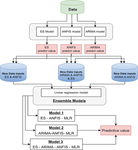
To better illustrate the proposed predictive system, a block diagram graphical representation is provided in Figure 2. The first phase of the proposed system entails the collection of data, as elucidated in section “Data”, and visualizing the time series of the gathered datasets. Subsequently, the data undergoes pre-processing, which is also illustrated in the initial phase of Figure 2. This phase involves essential data processing tasks, such as removing outliers, imputing missing values, and dividing the data into training and testing sets, before any future operations can occur.

Figure 2. Block diagram of the study.

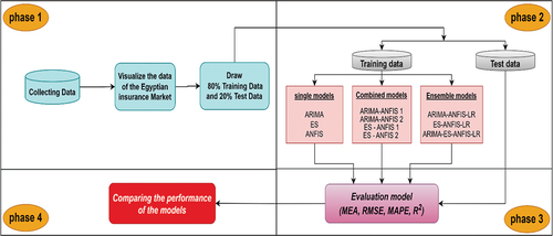
The second phase of Figure 2 incorporates two statistical time series models, specifically ARIMA and ES models, in addition to an artificial intelligence model, the ANFIS models, as well as combination models using two patterns relying on either the statistical models’ error or predicted values. In addition, the ensemble models use multi-linear regression models based on ARIMA, ES, and ANFIS in three patterns, combining the models in different ways, as delineated in section “Methodology”. In the third phase, the performance of all predictive models utilized in the study is evaluated using four evaluation measures, as discussed in section “Discussion on the evaluation metrics of forecasting models”. Finally, the results obtained using the combination and ensemble models are compared to those obtained using the individual models.

Overall, this block diagram provides a clear and concise overview of the proposed predictive system, detailing the various phases involved and the methods utilized at each phase of the process.

Discussion on the Evaluation Metrics of Forecasting Models

The evaluation of a model’s performance is dependent on its ability to generate forecast values that are closely aligned with the observed values for the test data. To compare the efficacy of the ARIMA, ES, ANFIS, and other combination and ensemble models used in this study, four distinct forecast consistency measures were utilized. Four statistical criteria, namely Mean Absolute Error (MAE), Mean Absolute Percent Error (MAPE), R Square (R²), and Root Mean Square Error (RMSE), were adopted as measures of forecasting accuracy to assess the models (Jain et al. 2019; Khalil et al. 2022; Wei et al. 2019), as defined in Equations (1)(1) $\mathit{MAPE}=\frac{100}{n}\sum _{\mathit{t}=1}^n\left|\frac{y_t-y_t^{\ast }}{y_t}\right|,$(1) -(4(4) $R^2=1-\frac{{\sum }_{t=1}^n{\left(y_t-y_t^{\ast }\right)}^2}{{\sum }_{t=1}^n{\left(y_t-{\bar{y}}_{\mathit{t}}\right)}^2},$(4) ), respectively. The measures are presented as follows:

(1) $\mathit{MAPE}=\frac{100}{n}\sum _{\mathit{t}=1}^n\left|\frac{y_t-y_t^{\ast }}{y_t}\right|,$(1)

(2) $\mathit{MAE}=\frac{1}{n}\sum _{\mathit{t}=1}^n\left|y_t-y_t^{\ast }\right|,$(2)

(3) $\mathit{RMSE}=\sqrt{\frac{1}{n}\sum _{\mathit{t}=1}^n{\left(y_t-y_t^{\ast }\right)}^2},$(3)

(4) $R^2=1-\frac{{\sum }_{t=1}^n{\left(y_t-y_t^{\ast }\right)}^2}{{\sum }_{t=1}^n{\left(y_t-{\bar{y}}_{\mathit{t}}\right)}^2},$(4)

where $y_t$ and $y_t^{\ast }$ denote actual and predicted model data samples, respectively. $\mathit{n}$ is the sample size. ${\bar{y}}_{\mathit{t}}$ is the average of actual data.

Methodology

In this section, the analytical techniques employed in the study are presented in detail, including any statistical or computational tools used. The goal of this section is to provide a clear and comprehensive account of the methods used to analyze the data.

The practice of forecasting time series is widely recognized as one of the most difficult applications of contemporary time series forecasting. Thus, we propose a framework that uses both statistical time series (ARIMA and ES models) and artificial intelligent approaches (ANFIS model), embedding them in a combination model and ensemble model for better results and to provide the decision Makers in insurance companies with more precise predictions. Each learning model is subjected to a grid search in order to obtain the best parameter tuning.

Statistical Time Series Methods

Autoregressive Integrated Moving Average Model (ARIMA)

The ARIMA model integrates autoregression and the moving average, which was introduced by Box and Jenkins (Box et al. 2015). The ARIMA model consists of three different levels: identification, parameter estimation, and prediction. At the level of identification, stationarity is validated for accuracy (Farsi et al. 2021). Data from non-stationary time series can be converted into data from stationary time series by differentiating or power transforming it (Choubin and Malekian 2017). Iterating this procedure d times results in a d-order integration of the model. In the next stage, the number of moving average terms (q) and the number of autoregressive terms (p) were then calculated using the graphical features of the autocorrelation function (ACF) and partial autocorrelation function (PACF). Finally, we estimate subsequent data values using historical ones as a guide (Geetha and Nasira 2016). The future value of a variable in an ARIMA model is assumed to be a linear mixture of previous values and past errors, expressed as follows:

(5) $y_t=a_0+\sum _{\mathit{i}=1}^p{\varphi }_i{y}_{\mathit{t}-1}+\sum _{\mathit{j}=0}^q{\varphi }_j{\epsilon }_{\mathit{t}-\mathit{j}},$(5)

where $y_t$ stationary is a stochastic process,$\mathit{\hspace{0.17em}}{a}_0$ is the constant, ${\epsilon }_t\mathit{\hspace{0.17em}}$ is the error or white noise disturbance term, ${\varphi }_i$ represents the auto-regression coefficient and ${\varphi }_j\mathit{\hspace{0.17em}}$is the moving average coefficient.

Obtaining reasonable estimates for p, q, and d is a significant obstacle when employing the ARIMA model. The data’s temporal correlation structure is identified by (ACF and PACF). Parameters of the ARIMA model can be chosen with the assistance of the ACF and PACF plots, but modelers should still try out various values for p, q, and d to obtain the best fit. In this article, the optimal values of parameters were selected according to the lowest values of the Akaike information criterion (AIC) and the Bayesian information criterion (BIC) measures for the ARIMA models values for predicting the retention ratio of Egyptian insurance market, where it is used to compare different models and select the best one for a given dataset (Farsi et al. 2021; Khozani et al. 2022). The AIC and BIC are defined as follows (Hyndman and Athanasopoulos 2021):

(6) $\mathit{AIC}=2\mathit{k}-\mathit{nln}\left(\mathit{L}\right),$(6)

(7) $\mathit{BIC}=\mathit{kIn}\left(\mathit{n}\right)-\mathit{nln}\left(\mathit{L}\right),$(7)

where $\mathit{L}\mathit{\hspace{0.17em}}=\mathit{\hspace{0.17em}}\mathit{L}\mathit{\hspace{0.17em}}\left(\hat{\theta }\right)$ is the maximum value of likelihood function of model, and k is the number of parameters and n is the number of observations in the dataset. As a final step, verifying the generation stop is performed. The optimal ARIMA parameter values may be obtained automatically using this method, which is a major plus. ARIMA models were executed in MATLAB (2022a).

Exponential Smooth Model (ES)

The term “ES” designates the adaptive techniques used to forecast time series. Because of its adaptive mechanism, ease of implementation, and straightforward interpretation of results, ES plays a significant role in insurance ratios forecasting. In insurance, computerized prediction utilizing a suite of exponential smoothing models has seen tremendous growth in popularity (Pires et al. 2022). Furthermore, ES denotes short-term forecasting methods, and the simplest model that does not incorporate trend and seasonal components is presented as follows:

(8) ${\hat{x}}_{\mathit{t}}=\mathit{\alpha }{x}_t+\left(1-\mathit{\alpha }\right){\hat{x}}_{\mathit{t}-1},$(8)

where $x_t$ is the value of the time series at time t; ${\hat{x}}_{\mathit{t}}$ is the predicted value of the time series at time t; $\mathit{\alpha }$ is the fixed exponential value between zero and one (smoothing coefficient) taken into consideration that the model is based on the value of (α) optimal. Due to the difficulty in obtaining its smoothing parameters, ES model may be ineffective if the system’s structure is unclear and there is insufficient data (Dudek, Pełka, and Smyl 2021).

The Adaptive Neuro-Fuzzy Inference System (ANFIS)

Adaptive Neuro-Fuzzy Inference System (ANFIS) is a type of neuro fuzzy system that combines the strengths of fuzzy logic (FL) and artificial neural networks (ANNs) introduced by Jang and implements the Takagi‐Sugeno inference system (Jang 1993). The Sugeno system has many advantages, such as being computationally effective and suitable to work with linear, optimization, and adaptive methods. It is designed to model and make predictions based on complex, non-linear relationships between input and output variables. ANFIS is a powerful tool for modeling and predicting real-world systems, as it can handle uncertainty and imprecise data. Thus, ANFIS models can be used for a wide range of applications, including time series prediction, classification, control, and decision-making. They have been applied to fields such as finance, engineering, environmental science, and medicine (Khalil, Liu, and Ali 2022).

ANFIS models are constructed by defining a set of membership functions (MF), which describe the fuzzy relationships between the inputs and outputs. The membership functions are then combined in a fuzzy inference system (FIS) to form the overall model. ANFIS models are trained using a combination of backpropagation and least-squares estimation algorithms, which allow the model to adjust the parameters of the membership functions to minimize the prediction error (Rathnayake et al. 2023).

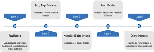
The ANFIS is a multi-layer model that consists of five layers, each of which serves a specific purpose in the overall functioning of the model as shown in Figure 3. The first layer is the input layer that accepts inputs, the second layer is the fuzzy layer, where fuzzy sets and membership functions are created. The third layer is the normalization layer, which normalizes the output of the fuzzy layer. The fourth layer is the rule layer, which generates the fuzzy rules based on the normalized output of the previous layer. Finally, the output layer is the fifth layer, which generates the output of the ANFIS model. When the ANFIS technique learns the membership functions from the training data, it also develops the system rules. It is a hybrid learning rule-based adaptive network. Assume that the FIS under consideration has two inputs x and y and one output S. With a Sugeno fuzzy model of the first order, the rule-base consists of two fuzzy if-then rules designated as follows (Jang 1993; Oroian 2015):

Figure 3. ANFIS structure for the sugeno fuzzy model.

(9) $\mathit{Rule}1:\mathit{If}{x}_1=A_1\mathit{and}{x}_2=C_1\mathit{then}{f}_1=n_1{x}_1+m_1{x}_2+r_1,$(9)

(10) $\mathit{Rule}2:\mathit{If}{x}_1=A_2\mathit{and}{x}_2=C_2\mathit{then}{f}_2=n_2{x}_1+m_2{x}_2+r_2,$(10)

where $x_1$ and $x_2$ are independent variables, $A_i$ and $C_i$ are fuzzy sets, and $n_i$, $m_i$, and $r_i$ are dependent variable parameters.

In conclusion, the ANFIS model is a powerful tool for modeling complex non-linear relationships between inputs and outputs. Each layer of the model serves a specific purpose, and the combination of these functions allows ANFIS to model complex relationships with high accuracy. Additionally, ANFIS models are relatively easy to implement and can be trained using widely available software tools, such as MATLAB and Python.

The Combination Models

Combining methods has proven to be effective in addressing the limitations of individual models and techniques. Through combining different models or techniques, the limitations of each method can be overcome, and a more comprehensive understanding of the data can be achieved (Jain et al. 2019).

In data of insurance ratios are rarely pure linear or nonlinear. The retention ratio data in insurance companies often contains both linear and nonlinear patterns, making it difficult to capture its behavior with a single universal model. Therefore, a combined strategy that incorporates both linear and nonlinear modeling abilities can be a better approach for forecasting retention ratio in the Egyptian insurance market. To achieve this, we use a combination of ARIMA and ES models to capture the linear information in the time series of retention ratio. Additionally, an ANFIS model is used to handle the non-linear pattern in the outputs of the ARIMA and ES models to capture the nonlinear information. Two methods for combining the individual predictions produced by the ARIMA, ES, and ANFIS models are considered as shown in Figure 4, in order to identify the optimal model for solving the forecasting problem.

Figure 4. The structure of proposed combination models.

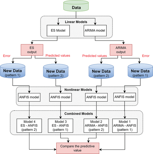
The ARIMA, ES, and ANFIS models have different capabilities in capturing data characteristics in linear or nonlinear domains. Thus, combining two or more models can provide a robust method with improved overall forecasting performance that can model both linear and nonlinear patterns. Our paper considers two methods for combining individual predictions produced by the ARIMA, ES, and ANFIS models relying on either the statistical models’ error or predicted values.

The first method involves calculating the difference between the actual and forecasted retention ratio obtained from the ARIMA and ES models, which is then used as a new input in the original dataset. The ANFIS model is then applied to this augmented dataset, which includes two inputs (time and statistical model’s error) and one output. Then, the combination method using a suitable ANFIS model is implemented. This method can be expressed mathematically as:

1. The errors $e_t$ between the actual and forecasted retention ratios produced by the ARIMA and ES models are calculated as:

   (11) $e_t=y_t-h_t,$(11)

   where $e_t$ is the error value, $y_t$ is the actual value of data, and $h_t$ is the forecasted values of statistical models.

2. The ANFIS model is used to forecast the retention ratio $y_t$ at time t based on the time variable and the errors $e_t$:

   (12) ${\hat{y}}_{\mathit{t}}=\mathit{ANFIS}\left(\mathit{t},e_t\right),$(12)

   where the ANFIS model can be represented as:

   (13) ${\hat{y}}_{\mathit{t}}=\mathit{f}\left(x_t,e_t\right)=\sum _{\left\{\mathit{i}=1\right\}}^m{w}_i{\phi }_{i\left(x_t,e_t\right)},$(13)

where $x_t$ is the time variable, $e_t$ is the error term, $w_i$ is the weight of the $\mathit{i}$ fuzzy rule, ${\phi }_i$is the $\mathit{i}$ fuzzy rule.

In the second method, the predicted values produced by the ARIMA and ES models is used as inputs for the ANFIS model. Specifically, the ARIMA and ES models are applied first to forecast the retention ratio of the Egyptian insurance market, then take the predicted values produced by these models as inputs for the ANFIS model, which has one output (retention ratio) and two inputs (time and predicted values from ARIMA and ES models). The ANFIS model then produces the final prediction of the retention ratio. Mathematically, we can represent the second method as follows:

(14) ${\hat{y}}_{\mathit{t}}=\mathit{f}\left(x_t,h_t\right)=\sum _{\left\{\mathit{i}=1\right\}}^m{w}_i{\phi }_{i\left(x_t,h_t\right)},$(14)

where ${\hat{y}}_{\mathit{t}}$ represents the final prediction of the retention ratio at time t, and $x_t$ is the time variable, $h_t$ is predicted values from ARIMA and ES models, $w_i$ is the weight of the $\mathit{i}$ fuzzy rule, ${\phi }_i$is the $\mathit{i}$ fuzzy rule.

The Ensemble Models

Ensemble forecasting is a technique for enhancing the accuracy and reliability of forecasting by stacking multiple outputs from diverse forecasting models. Recent studies have demonstrated the efficacy of integrating multiple models into an ensemble in terms of robustness and reliability (Aras 2021). For ensemble results, two methods are commonly used: averaging and stacking. However, this study will focus on the stacking approach.

Stacking is a general method that involves combining a higher-level model with lower-level models in order to achieve greater predictive accuracy (Akyol 2020). In this approach, all models including ARIMA, ES, and ANFIS are integrated into an ensemble model through three patterns, as depicted in Figure 5. These models are fed identical input values, with the output of each model serving as independent predictors for the combined model. To ascertain the weight of the contribution of these predictors, multi-linear regression is performed between them. Therefore, the final output of the ensemble model can be expressed as follows:

Figure 5. The structure of proposed ensemble models.

(15) ${\hat{H}}_{\mathit{t}}=B_0+{\beta }_1{F}_t^{m1}+{\beta }_2{F}_t^{m2}+\dots +{\beta }_i{F}_t^{mi},$(15)

where ${\hat{H}}_{\mathit{t}}$ is the predicted value of the ensemble model at time t, $F_t^m$ denotes the input of the individual models (predictive values), where $\mathit{m}\in \left\{\mathit{ARIMA},\mathit{\hspace{0.17em}}\mathit{ES},\mathit{ANFIS}\right\}$, and The weights assigned to each predictor are represented by$\mathit{\hspace{0.17em}}{\beta }_1,\mathit{\hspace{0.17em}}{\beta }_2,\mathit{\hspace{0.17em}}\mathit{and}\mathit{\hspace{0.17em}}{\beta }_3,\mathit{\hspace{0.17em}}\mathit{and}\mathit{\hspace{0.17em}}{\beta }_0\mathit{\hspace{0.17em}}$is the intercept. The goal of the regression analysis is to determine the value of the coefficients that provide the best fit to the observed data.

In conclusion, the section discusses the analytical techniques employed in the study for time series forecasting, which includes statistical time series and AI approaches. The proposed framework uses a combination model and ensemble model that embeds both approaches to achieve better results. The statistical time series methods discussed in the study are ARIMA and ES, as well as ANFIS as AI model. The section provides detailed explanations of the ARIMA, ES and ANFIS models, including equations and the identification and parameter estimation levels. Additionally, the section highlights the proposed framework of the combination and ensemble models. Finally, the section mentions that MATLAB software was used to run the models in the study.

Results and Discussion

In this section, the forecasting findings are computed utilizing the presented predictive models and comparisons to other models, as well as the discussion of the results are also included.

Statistical Time Series Models

In this study, two conventional statistical time series models are implemented. For the simulation, Econometric Package in MATLAB was used. Econometric Package is a complete and useful statistical analysis too. The application process for the ARIMA and ES models is described in detail. Table 2 shows the optimal parameters of Statistical time series models.

Table 2. The optimal parameters of statistical time series models.

Model	Parameters	Optimal values
ARIMA	AR (p) I (d) MA (q) The innovation distribution function	p = 2 d = 1 q = 1 Gaussian Distribution
ES	ALPHA (α)	α= 0.9999

For ARIMA model, the Autocorrelation Function (ACF) and Partial Autocorrelation Function (PACF) of the data are graphically represented as illustrated in Figure 6. The ACF provides insight into the linear relationship between the data and its lagged values, essentially depicting the extent of correlation between data points separated by various time lags. On the other hand, the PACF illustrates the correlation between data points separated by specific time lags while controlling for any correlation attributable to the intervening data points. These graphical representations, as showcased in Figures 6 and 7, clarify the ACF and PACF for ARIMA (2,1,1) model. According to that many ARIMA models are applied, and AIC and BIC measures were chosen to determine the best ARIMA model for observed data as shown in Table 3. The ARIMA (2, 1, 1) is the best fit model which gets the lowest values of AIC and BIC.

Figure 6. The plot of (ACF & PACF) of the market time series.

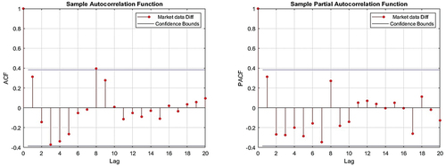
Figure 7. The plot of the ARIMA (2,1,1) model fit.

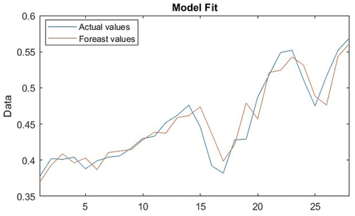
Table 3. The goodness of fit measure of ARIMA models.

	The measure
Model	AIC	BIC	Parameters significance
ARIMA (1,0,1)	−121.07	−115.89	AR MA	Significant Not Significant
ARIMA (1,1,1)	−121.02	−115.99	AR MA	Not Significant Not Significant
ARIMA (1,1,2)	−126.20	−119.91	AR MA	Significant Not significant
ARIMA (2,1,1)	−130.89	−124.80	AR MA	Significant Significant
ARIMA (2,1,2)	−129.30	−123.06	AR MA	Significant Not significant

The estimated parameters for ARIMA (2,1,1) model are summarized in Table 4. The table shows that at a 5% significance level. In addition, the accuracy measure for the best ARIMA model for training and testing data were MAE = 0.0144, RMSE = 0.0194, and MAPE = 3.222, for training data and MAE = 0.0246, RMSE = 0.0307, and MAPE = 4.219, for testing data, as well as R² for the model was 0.885, as presented in Table 5. Figure 8 demonstrates that the residuals originating from the ARIMA (2,1,1) model conform to a normal distribution. This implies that the disparities between the anticipated values of the model and the real observed values, denoted as residuals, are distributed in a manner that conforms to a bell-shaped curve or Gaussian distribution. This pattern suggests that the model is sufficiently capable of capturing the fundamental structure of the data.

Figure 8. The plots of residual normality of ARIMA (2,1,1) model.

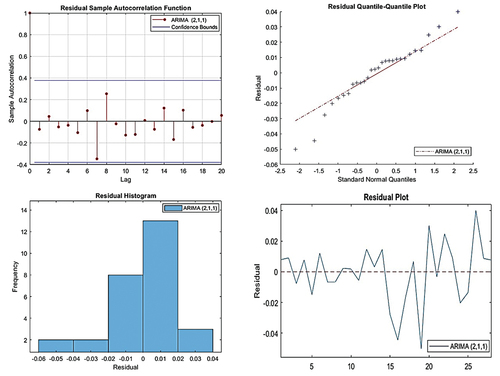
Table 4. The parameters of the ARIMA (2,1,1) model.

Parameters	Value	Standard Error	T Statistic	P-Value
Constant	0.00284	0.0011	2.5808	0.0098
AR {1}	1.07050	0.1731	6.1841	0.0000
AR {2}	−0.5679	0.1476	−3.8471	0.0001
MA {1}	–1	0.1811	–5.5199	0.0000
Variance	0.00038	0.0001	2.6323	0.0084

Table 5. The accuracy measure of the best ARIMA and ES models.

	MAE		RMSE		MAPE
Model	Train	Test	Train	Test	Train	Test	R^2
ARIMA (2,1,1)	0.0144	0.0246	0.0194	0.0307	3.222	4.219	0.885
ES (α= 0.9999)	0.0203	0.0202	0.0264	0.0232	4.383	3.584	0.795

For exponential smoothing model (ES), As mentioned in Table 2 the best parameter for the model is Alpha = 0.999, and the accuracy measure for ES model for training and testing data were MAE = 0.0.203, RMSE = 0.0264, and MAPE = 4.383, for training data and MAE = 0.0202, RMSE = 0.0232, and MAPE = 3.584, for testing data, as well as R² for the model was 0.795, as presented in Table 5. Figure 9 shows how well the ES (Exponential Smoothing) model suited the training set of data. In order to assess the model’s effectiveness and fitness for additional analytical or forecasting tasks, it is critical to see how closely the model’s predictions match the actual values in the training dataset.

Figure 9. The plot of the ES model fit.

ANFIS Model

ANFIS models are created using the fuzzy designer tool in MATLAB. A wide variety of ANFIS models with inputs and outputs of the MF type and optimal train FIS techniques are applied to the observed data. The rule-based connection between the input and output variables was set up using a grid fuzzy partition. As inputs, we have chosen the triangular function (Trimf), the Gaussian curve (Gaussmf), the trapezoidal function (Tramf), and the Gaussian combination function (Gauss2mf). then constant and linear output types are employed. As the optimal train, the FIS technique hybrid is used. Table 6 shows the optimal ANFIS model parameters.

Table 6. The parameters of the best ANFIS model.

	M.F type		M.F number
Model	Input	Output		ANFIS Info
ANFIS (5)	Gaussian	Linear	8	Number of Nodes	36
				Linear Parameter	8
				Non-linear Parameter	32
				Total Parameter	40
				Fuzzy Rules	8

The results are described in the following discussion. Both the time data and the actual value were used in the process. The ANFIS model with the lowest MAE, RMSE, and MAPE was chosen. According to Table 7, the best-performing FIS model was the ANFIS model (5), which used a Gaussian membership function for inputs, linear outputs, eight membership functions for inputs, and a hybrid technique for training FIS. Figure 10 presents the Trained Membership Functions, the architecture of the ANFIS model, and the error associated with the model (5) as it relates to the epoch count. It is evident from the figure that the error diminishes until approximately 494 epochs are reached, post which the error levels plateau and remain almost unchanged. The graph indicates an optimization in error reduction until a certain number of iterations (epochs), beyond which additional training does not significantly improve the model’s performance.

Figure 10. Trained membership functions and the structure of ANFIS model.

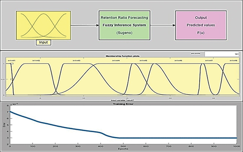
Table 7. The accuracy measure of ANFIS model.

	M.F. type			Train FIS		MAE		RMSE		MAPE
Model	Input	Output	No. MF	Optimal. Method	Epoch	Train	Test	Train	Test	Train	Test	R^2
1	Trimf	linear	5	hybrid	500	0.0054	0.0159	0.0073	0.0201	1.249	2.815	0.978
2		constant	6		1000	0.0084	0.0120	0.0135	0.0164	1.822	2.185	0.979
3	Trapmf	linear	3	hybrid	1500	0.0126	0.0270	0.0193	0.0318	2.811	4.636	0.910
4		constant	4		2500	0.0101	0.0238	0.0169	0.0267	2.202	4.114	0.933
5	Gaussmf	linear	8	hybrid	1000	0.0022	0.0119	0.0029	0.0131	0.492	2.118	0.993
6		constant	8		3500	0.0038	0.0144	0.0056	0.0177	0.866	2.498	0.985
7	Gauss2mf	linear	3	hybrid	1500	0.0105	0.0274	0.0170	0.0325	2.218	4.713	0.924
8		constant	8		2000	0.0024	0.0116	0.0038	0.0163	0.538	2.035	0.988

The Combined Methods

As we mentioned in section “The combination models”, two patterns of combination method are implemented in this study. The first method involves calculating the difference between the actual and forecasted retention ratio obtained from the ARIMA and ES models, which is then used as a new input in the original dataset. The ANFIS model is then applied to this augmented dataset, which includes two inputs (time and statistical model’s error) and one output. Then, the combination method using a suitable ANFIS model is implemented. In the second method, the predicted values produced by the ARIMA and ES models are used as inputs for the ANFIS model. Specifically, the ARIMA and ES models are applied first to forecast the retention ratio of the Egyptian insurance market. Then, the predicted values produced by these models are used as inputs for the ANFIS model.

The first combination approach, which makes use of the residuals from the ARIMA model, yielded the outcomes displayed in Tables 8. Utilizing a Gaussian combination member function (Gauss2mf) for its inputs, constant outputs, with 10 and 2 membership functions for first and second input, respectively, and a hybrid method for train FIS, model number (8) of the ANFIS models was found to be the best model for testing data. As shown in Figure 11, the variation of error of model (8) with increasing epoch numbers, it found that errors continue to diminish until approximately 50 epochs, before becoming almost constant.

Figure 11. The variation of error and the structure of ARIMA-ANFIS model for pattern (1).

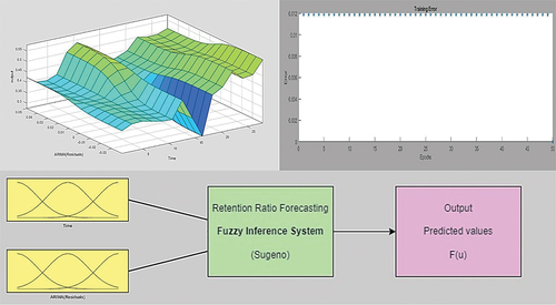
Table 8. The accuracy measure of first pattern of combined model (ARIMA-ANFIS).

	M.F. type			Train FIS		MAE		RMSE		MAPE
Model	Input	Output	No. MF	Optimal. Method	Epoch	Train	Test	Train	Test	Train	Test
1	Trimf	Linear	5.5	hybrid	50	3.2E–5	0.0631	6.2E–5	0.0743	0.008	11.12
2		Constant	4.2		50	0.0170	0.0109	0.0224	0.0142	3.732	1.893
3	Trapmf	Linear	2.2	hybrid	50	0.0152	0.0494	0.0203	0.0564	3.420	8.609
4		Constant	3.2		50	0.0153	0.0167	0.0193	0.0195	3.380	2.879
5	Gaussmf	Linear	4.6	hybrid	50	3.5E–5	0.0355	7.4E–5	0.0447	0.008	6.321
6		Constant	9.2		50	0.0058	0.0110	8.7E–3	0.0152	1.213	1.917
7	Gauss2mf	Linear	6.4	hybrid	50	1.6E–5	0.0153	2.8E–5	0.0211	0.004	2.727
8		Constant	10.2		50	0.0089	0.0108	0.0119	0.0136	2.009	1.884

The results of the combination model using ES model’s residuals showed that model number (8) were the best model for testing data, utilizing a Gaussian combination membership function (Gauss2mf) for its inputs, constant outputs, with 3 membership functions for each input, and a hybrid method for train FIS. Figure 12 displays the error of model (8) as a function of epoch number, showing that errors decrease until around 50 epochs, after which they remain nearly constant. Table 9 summarizes the ANFIS model results and specifications.

Figure 12. The variation of error and the structure of ES-ANFIS model for pattern (1).

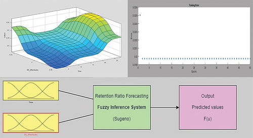
Table 9. The accuracy measure of first pattern of combined model (ES-ANFIS).

	M.F. type			Train FIS		MAE		RMSE		MAPE
Model	Input	Output	No. MF	Optimal. Method	Epoch	Train	Test	Train	Test	Train	Test
1	Trimf	Linear	8.6	hybrid	50	7.9E–8	0.0563	1.6E–7	0.0680	1.9E–5	9.957
2		Constant	4.2		50	0.0181	0.0127	0.0229	0.0173	3.979	2.212
3	Trapmf	Linear	5.3	hybrid	50	2.5E–4	0.0481	4.6E–4	0.0562	0.059	8.423
4		Constant	3.3		50	0.0152	0.0122	0.0200	0.0176	3.405	2.090
5	Gaussmf	Linear	4.6	hybrid	50	2.6E–5	0.0526	5.3E–5	0.0659	0.006	9.279
6		Constant	9.2		50	0.0037	0.0124	5.5E–3	0.0171	0.819	2.165
7	Gauss2mf	Linear	3.3	hybrid	50	0.0043	0.0145	5.7E–3	0.0193	0.984	2.551
8		constant	3.3		50	0.0155	0.0096	0.0199	0.0148	3.470	1.635

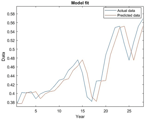
For the second combination method with using statistical methods’ predicted values as input. Table 10 shows that using the predicted values of the ARIMA model, the best model for testing data was model number (5), which used a Gaussian membership function (Gaussmf) as inputs, linear outputs, 6 and 4 membership functions for first and second inputs, respectively, and a hybrid method to train FIS. Figure 13 depicts the errors of model (5) as a function of epoch number, showing that errors decrease with time up to around 50 epochs, after which they remain nearly constant.

Figure 13. The variation of error and the structure of ARIMA-ANFIS model for pattern (2).

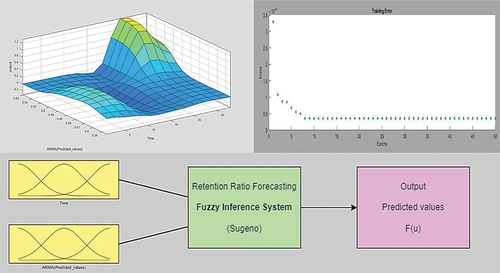
Table 10. The accuracy measure of second pattern of combined model (ARIMA-ANFIS).

	M.F. type			Train FIS		MAE		RMSE		MAPE
Model	Input	Output	No. MF	Optimal. Method	Epoch	Train	Test	Train	Test	Train	Test
1	Trimf	Linear	5.3	hybrid	50	7.9E–4	0.0254	1.4E–3	0.0269	0.189	4.443
2		constant	2.2		50	0.0144	0.0170	0.0188	0.0234	3.195	2.908
3	Trapmf	Linear	4.7	hybrid	50	7.5E–4	0.0324	1.5E–3	0.0437	0.178	5.602
4		constant	2.3		50	0.0120	0.0201	0.0180	0.0264	2.684	3.440
5	Gaussmf	Linear	6.4	hybrid	50	2.1E–5	0.0105	3.5E–5	0.0154	0.005	1.831
6		constant	10.2		50	0.0027	0.0119	0.0040	0.0164	0.604	2.092
7	Gauss2mf	Linear	2.9	hybrid	50	0.0003	0.0224	6.5E–4	0.0263	0.071	3.896
8		constant	10.4		50	0.0011	0.1198	1.9E–3	0.1718	0.253	20.73

According to Table 11, the results of the combination model using ES model’s predicted values showed that model number (7) of were the best model for testing data, which used a Gaussian combination membership function (Gauss2mf) for its inputs, linear outputs, and 2 membership functions for each input, and a hybrid technique to train FIS. Figure 14 displays the error variation of model (2) as epochs increase, showing that errors decrease until about epoch 50, after which they remain nearly constant.

Figure 14. The variation of error and the structure of ES-ANFIS model for pattern (2).

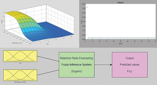
Table 11. The accuracy measure of second pattern of combined model (ES-ANFIS).

	M.F. type			Train FIS		MAE		RMSE		MAPE
Model	Input	Output	No. MF	Optimal. Method	Epoch	Train	Test	Train	Test	Train	Test
1	Trimf	Linear	6.2	hybrid	50	4.9E–4	0.0238	7.0E–4	0.0283	0.115	4.087
2		Constant	6.6		50	1.8E–3	0.0114	3.3E–3	0.0163	0.455	2.001
3	Trapmf	Linear	2.2	hybrid	50	0.0136	0.0169	0.0178	0.0198	2.962	2.914
4		Constant	4.4		50	0.0134	0.0198	0.0189	0.0228	3.039	3.403
5	Gaussmf	Linear	8.2	hybrid	50	1.4E–4	0.0257	1.9E–4	0.0299	0.032	4.433
6		Constant	10.6		50	3.4E–6	0.0175	6.6E–6	0.0163	8.2E–4	2.055
7	Gauss2mf	Linear	2.2	hybrid	50	0.0118	0.0109	0.0166	0.0137	2.544	1.912
8		Constant	10.10		50	1.9E–6	0.0122	2.8E–6	0.0166	4.5E–4	2.119

The Ensemble Methods

As we mentioned in section “The ensemble models”, three models of ensemble method are implemented in this study, including ARIMA, ES, and ANFIS as depicted in Figure 5. These models are fed identical input values, with the output of each model serving as independent predictors for the combined model. To ascertain the weight of the contribution of these predictors, multi-linear regression is performed between them.

Table 12 shows the results of the three ensemble models and the model 1 which used the predicted values of ARIMA, ES and ANFIS models was the best model for testing data and the accuracy measures of this model were MAE = 0.0095, RMSE = 0.0101, and MAPE = 1.651, as well as R² for the model was 0.9956.

Table 12. The accuracy measure of ensemble models.

		MAE		RMSE		MAPE
No	Model	Train	Test	Train	Test	Train	Test	R^2
1	ARIMA - ES - ANFIS – MLR	2.16E–3	0.0095	2.76E–3	0.0101	0.489	1.651	0.9956
2	ARIMA - ANFIS – MLR	2.16E–3	0.0131	2.77E–3	0.0140	0.488	2.300	0.9933
3	ES - ANFIS – MLR	2.15E–3	0.0572	2.87E–3	0.0586	0.487	10.00	0.9583

According to the results in Table 13, it was found that among the single predictive models, the ANFIS model had the best performance for the testing data based on four predictive performance indicators: MAE, RMSE, MAPE, and R², with values of 0.0119, 0.0161, 2.118 and 0.993 respectively, as shown in Figure 15(a). The proposed combined and ensemble models were also evaluated, and the results showed that the first pattern of combined model (ES-ANFIS) outperformed the other combined models, having lower values of MAE, and MAPE at 0.0096 and 1.1665, respectively, as shown in Figure 15(b). In conclusion, Table 13 reveals that the ensemble model (ARIMA-ES-ANFIS-MLR) had the best overall performance in predicting retention ratio of the Egyptian insurance market, compared to all other models, as it had lower values of MAE, RMSE, MAPE, and R², with values of 0.0095, 0.0101, 1.651, and 0.9956, respectively, as shown in Figure 15(c).

Figure 15. The comparison of all predictive models (a) single models (b) combined models (c) ensemble models.

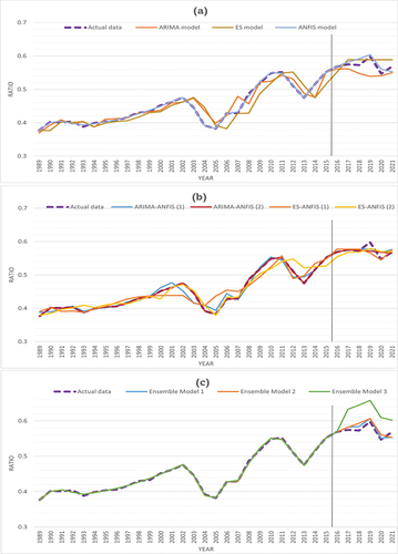
Table 13. The comparison between all the models.

		MAE		RMSE		MAPE
Model		Train	Test	Train	Test	Train	Test	R^2	Order
Single models	ARIMA	0.0144	0.0246	0.0194	0.0307	3.222	4.219	0.885	9^th
	ES	0.0203	0.0202	0.0264	0.0232	4.383	3.584	0.795	8^th
	ANFIS	2.2E–3	0.0119	2.9E–3	0.0161	0.492	2.118	0.993	6^th
Combined models	ARIMA-ANFIS (pattern 1)	0.0089	0.0108	0.0119	0.0136	2.009	1.884	0.959	4^th
	ES-ANFIS (pattern 1)	0.0155	0.0096	0.0199	0.0148	3.470	1.665	0.881	2^nd
	ARIMA-ANFIS (pattern 2)	2.1E–5	0.0105	3.5E–5	0.0154	0.005	1.831	0.997	3^rd
	ES-ANFIS (pattern 2)	0.0118	0.0109	0.0166	0.0137	2.544	1.912	0.917	5^th
Ensemble models	ARIMA- ES - ANFIS - MLR	2.1E–3	0.0095	2.7E–3	0.0101	0.487	1.651	0.996	1^st
	ARIMA - ANFIS - MLR	2.16E–3	0.0131	2.77E–3	0.0140	0.488	2.300	0.993	7^th
	ES - ANFIS - MLR	2.15E–3	0.0572	2.87E–3	0.0586	0.487	10.00	0.958	10^th

Conclusion

Improving the retention ratio prediction accuracy is of great significance for insurance companies’ decision makers and those interested in developing insurance services. Researchers in a range of fields aim to achieve accurate and reliable forecasting results, with the accuracy of time series forecasting being especially crucial in the insurance sector, which will assist insurance companies to address the effects of inflation and evaluate underwriting profitability, making reliable projection of future underwriting profits possible. The dataset utilized in this study was meticulously gathered from the annual records of the Egyptian property-liability insurance sector, as publicly disclosed by the Egyptian Financial Supervisory Authority (EFSA).

Recent academic research has shown a growing interest in the combination of predictive methods with ensemble techniques. This study enhances the current field by presenting four different combination models: ARIMA-ANFIS 1, ARIMA-ANFIS 2, ES-ANFIS 1, and ES-ANFIS 2, each representing diverse aggregation patterns. Three advanced ensemble models are used to predict the retention ratio in the Egyptian insurance market. Evaluation metrics such as MAE, RMSE, MAPE, and R2 are used to assess the effectiveness of the suggested models on both linear and nonlinear data connections. The results show that combining several approaches improves predictive accuracy by reducing the effects of randomness, temporal volatility, and nonlinearity in the dataset. The ensemble model, which combines ARIMA, ES, and ANFIS models using multi-linear regression, demonstrates strong performance, outperforming the separate and integrated models. These findings highlight the possibility of integrating ANFIS with well-known statistical time series approaches such as ARIMA and ES, as well as other ensemble techniques, to provide better forecasting capabilities for pertinent predictive problems.

This study presents a mathematical method that can accurately calculate an important insurance ratio. These endeavors promote comprehension and application of such methods in various situations. We suggest utilizing the approaches presented in this work to predict key ratios of other insurance companies in future studies. It excels at forecasting insurance time series data.

Authors’ Contributions

A. K. performed conceptualization, formal analysis, methodology, software, validation, visualization, and writing, reviewing & editing original draft. Z. L. preformed conceptualization, supervision, project administration, reviewing and editing the study. A. A. performed formal analysis, funding acquisition, reviewing and editing. All the authors have read and agreed to the submitted version of the manuscript.

Data Availability Statement

The data that support the findings of this study are publicly available on their website (https://fra.gov.eg).

Disclosure Statement

No potential conflict of interest was reported by the author(s).

Supplementary material

Supplemental data for this article can be accessed online at https://doi.org/10.1080/08839514.2024.2348413.

Additional information

Funding

This study is supported via funding from Prince Sattam bin Abdulaziz University project number [PSAU/2024/R/1445].

References

- Acakpovi, A., A. Tettey Ternor, N. Yaw Asabere, P. Adjei, and A.-S. Iddrisu. 2020. Time series prediction of electricity demand using adaptive neuro-fuzzy inference systems. Mathematical Problems in Engineering 2020:1–37. doi:10.1155/2020/4181045.
- Adnan, R. M., X. Yuan, O. Kisi, and V. Curtef. 2017. Application of time series models for streamflow forecasting. Civil and Environmental Research 9 (3):56–63. doi:10.7176/CER.
- Akyol, K. 2020. Stacking ensemble based deep neural networks modeling for effective epileptic seizure detection. Expert Systems with Applications 148:113239. doi:10.1016/j.eswa.2020.113239.
- Aras, S. 2021. Stacking hybrid GARCH models for forecasting bitcoin volatility. Expert Systems with Applications 174:114747. doi:10.1016/j.eswa.2021.114747.
- Arora, S., and A. K. Keshari. 2021. ANFIS-ARIMA modelling for scheming Re-aeration of hydrologically altered rivers. Journal of Hydrology 601:126635. doi:10.1016/j.jhydrol.2021.126635.
- Asadollahfardi, G., H. Zangooi, M. Asadi, M. Tayebi Jebeli, M. Meshkat-Dini, and N. Roohani. 2018. Comparison of box-jenkins time series and ANN in predicting total dissolved solid at the Zāyandé-Rūd River, Iran. Journal of Water Supply: Research and Technology-Aqua 67 (7):673–84. doi:10.2166/aqua.2018.108.
- Azadeh, A., M. Zarrin, H. Rahdar Beik, and T. Aliheidari Bioki. 2015. A neuro-fuzzy algorithm for improved gas consumption forecasting with economic, environmental and IT/IS indicators. Journal of Petroleum Science and Engineering 133:716–39. doi:10.1016/j.petrol.2015.07.002.
- Barak, S., and S. Saeedeh Sadegh. 2016. Forecasting energy consumption using ensemble ARIMA–ANFIS hybrid algorithm. International Journal of Electrical Power & Energy Systems 82:92–104. doi:10.1016/j.ijepes.2016.03.012.
- Bokaba, T., W. Doorsamy, and B. Sena Paul. 2022. A comparative study of ensemble models for predicting road traffic congestion. Applied Sciences 12 (3):1337. doi:10.3390/app12031337.
- Box, G. E. P., G. M. Jenkins, G. C. Reinsel, and G. M. Ljung. 2015. Time series analysis: Forecasting and control, 712. Hoboken, New Jersey: John Wiley & Sons.
- Cappiello, A. 2020. Risks and control of insurance undertakings. In The european insurance industry: Regulation, risk management, and internal control, ed. A. Cappiello, 7–29. Cham: Springer International Publishing.
- Chen, J.-F., Q. Hung Do, T. Van Anh Nguyen, and T. Thanh Hang Doan. 2018. Forecasting monthly electricity demands by wavelet neuro-fuzzy system optimized by heuristic algorithms. Information 9 (3):51. doi:10.3390/info9030051.
- Choubin, B., and A. Malekian. 2017. Combined gamma and M-Test-Based ANN and ARIMA models for groundwater fluctuation forecasting in semiarid regions. Environmental Earth Sciences 76 (15):1–10. doi:10.1007/s12665-017-6870-8.
- Choudhury, A., and J. Jones. 2014. Crop yield prediction using time series models. Journal of Economics and Economic Education Research 15 (3):53–67.
- Dewan, M. W., D. J. Huggett, T. Warren Liao, M. A. Wahab, and A. M. Okeil. 2016. Prediction of tensile strength of friction stir weld joints with Adaptive Neuro-Fuzzy Inference System (ANFIS) and neural network. Materials & Design 92:288–99. doi:10.1016/j.matdes.2015.12.005.
- Dudek, G., P. Pełka, and S. Smyl. 2021. A hybrid residual dilated LSTM and exponential smoothing model for midterm electric load forecasting. IEEE Transactions on Neural Networks and Learning Systems 33 (7):2879–91. doi:10.1109/TNNLS.2020.3046629.
- Fachini, F., and B. I. L. Lopes. 2019. Critical bus voltage mapping using anfis with regards to max reactive power in pv buses. 2019 IEEE Milan PowerTech, Milan, Italy, 1–6. IEEE. doi:10.1109/PTC.2019.8810562.
- Farsi, M., D. Hosahalli, B. R. Manjunatha, I. Gad, E.-S. Atlam, A. Ahmed, G. Elmarhomy, M. Elmarhoumy, and O. A. Ghoneim. 2021. Parallel genetic algorithms for optimizing the SARIMA model for better forecasting of the NCDC weather data. Alexandria Engineering Journal 60 (1):1299–316. doi:10.1016/j.aej.2020.10.052.
- Fu, W., P. Fang, K. Wang, Z. Li, D. Xiong, and K. Zhang. 2021. Multi-step ahead short-term wind speed forecasting approach coupling variational mode decomposition, improved beetle antennae search algorithm-based synchronous optimization and volterra series model. Renewable Energy 179:1122–39. doi:10.1016/j.renene.2021.07.119.
- Geetha, A., and G. M. Nasira. 2016. Time-series modelling and forecasting: Modelling of rainfall prediction using ARIMAmodel. International Journal of Society Systems Science 8 (4):361–72. doi:10.1504/IJSSS.2016.081411.
- Hasanov, M., M. Wolter, and E. Glende. 2022. Time series data splitting for short-term load forecasting. In PESS + PELSS 2022, 1–6. Kassel, Germany: Power and Energy Student Summit.
- Hasibuan, A. F. P., I. Sadalia, and I. Muda. 2020. The effect of claim ratio, operational ratio and retention ratio on profitability performance of insurance companies in Indonesia stock exchange. International Journal of Research and Review 7 (3):223–31. doi:10.52403/ijrr.
- He, W. 2017. Load forecasting via deep neural networks. Procedia Computer Science 122:308–14. doi:10.1016/j.procs.2017.11.374.
- Hu, Y., H. Zhang, C. Li, S. Liu, and Y. Zhang. 2013. Exponential smoothing model for condition monitoring: A case study. 2013 International Conference on Quality, Reliability, Risk, Maintenance, and Safety Engineering (QR2MSE), Chengdu, China, 1742–46. IEEE. doi:10.1109/QR2MSE.2013.6625913.
- Hyndman, R. J., and G. Athanasopoulos. 2021. Forecasting: principles and practice. Melbourne, Australia: OTexts. OTexts. Com/Fpp2. accessed 19.
- Jain, R., J. A. Alzubi, N. Jain, and P. Joshi. 2019. Assessing risk in life insurance using ensemble learning. Journal of Intelligent & Fuzzy Systems 37 (2):2969–80. doi:10.3233/JIFS-190078.
- Jang, J. S. 1993. ANFIS: adaptive-network-based fuzzy inference system. IEEE Transactions on Systems, Man, and Cybernetics 23 (3):665–85. doi:10.1109/21.256541.
- Joseph, V. R. 2022. Optimal ratio for data splitting. Statistical Analysis and Data Mining: The ASA Data Science Journal 15 (4):531–38. doi:10.1002/sam.11583.
- Joseph, V. R., and A. Vakayil. 2022. Split: an optimal method for data splitting. Technometrics 64 (2):166–76. doi:10.1080/00401706.2021.1921037.
- Kahloot, K. M., and P. Ekler. 2021. Algorithmic splitting: a method for dataset preparation. IEEE Access 9:125229–37. doi:10.1109/ACCESS.2021.3110745.
- Karia, A. A., I. Bujang, and I. Ahmad. 2013. Fractionally integrated ARMA for crude palm oil prices prediction: Case of potentially overdifference. Journal of Applied Statistics 40 (12):2735–48. doi:10.1080/02664763.2013.825706.
- Kaur, J., and P. Bassi. 2022. ‘Predictive performance of Indian insurance industry using artificial neural network (ANN) and support vector machine (SVM): A comparative study’. In Big data: A game changer for insurance industry, 65–79. Leeds: Emerald Publishing Limited. doi:10.1108/978-1-80262-605-620221005.
- Khademi, F., S. Mohammadmehdi Jamal, N. Deshpande, and S. Londhe. 2016. Predicting strength of recycled aggregate concrete using artificial neural network, adaptive neuro-fuzzy inference system and multiple linear regression. International Journal of Sustainable Built Environment 5 (2):355–69. doi:10.1016/j.ijsbe.2016.09.003.
- Khalil, A. A., Z. Liu, and A. A. Ali. 2022. Using an adaptive network‐based fuzzy inference system model to predict the loss ratio of petroleum insurance in Egypt. Risk Management and Insurance Review 25 (1):5–18. doi:10.1111/rmir.12200.
- Khalil, A. A., Z. Liu, A. Salah, A. Fathalla, and A. Ali. 2022. Predicting insolvency of insurance companies in Egyptian market using bagging and boosting ensemble techniques. IEEE Access 10:117304–14. doi:10.1109/ACCESS.2022.3210032.
- Khashei, M., and M. Bijari. 2011. A novel hybridization of artificial neural networks and ARIMA models for time series forecasting. Applied Soft Computing 11 (2):2664–75. doi:10.1016/j.asoc.2010.10.015.
- Khozani, Z. S., F. Barzegari Banadkooki, M. Ehteram, A. Najah Ahmed, and A. El-Shafie. 2022. Combining autoregressive integrated moving average with long short-term memory neural network and optimisation algorithms for predicting ground water level. Journal of Cleaner Production 348:131224. doi:10.1016/j.jclepro.2022.131224.
- Kuzu, Y., and A. L. P. Selçuk. 2022. Estimating the macroeconomic indicators using ARIMA and ANFIS methods. Recent Advances in Science and Engineering 2 (1). doi:10.14744/rase.2022.0002.
- Lai, K. K., L. Yu, S. Wang, and W. Huang. 2006. Hybridizing exponential smoothing and neural network for financial time series predication. Computational Science–ICCS 2006: 6th International Conference, Reading, UK, Springer, May 28-31, 493–500. Proceedings, Part IV 6.
- Lee, H.-H., and C.-Y. Lee. 2012. An analysis of reinsurance and firm performance: Evidence from the Taiwan property-liability insurance industry. The Geneva Papers on Risk and Insurance - Issues and Practice 37 (3):467–84. doi:10.1057/gpp.2012.9.
- Liu, Z., P. Jiang, L. Zhang, and X. Niu. 2020. A combined forecasting model for time series: Application to short-term wind speed forecasting. Applied Energy 259:114137. doi:10.1016/j.apenergy.2019.114137.
- Majid, R., and S. Ahmad Mir. 2018. Advances in statistical forecasting methods: An overview. Economic Affairs 63 (4):815–31. doi:10.30954/0424-2513.4.2018.5.
- Ma, C., L. Tan, and X. Xu. 2020. Short-term traffic flow prediction based on genetic artificial neural network and exponential smoothing. Promet-Traffic&Transportation 32 (6):747–60. doi:10.7307/ptt.v32i6.3360.
- Matloob, F., T. M. Ghazal, N. Taleb, S. Aftab, M. Ahmad, M. Adnan Khan, S. Abbas, and T. Rahim Soomro. 2021. Software defect prediction using ensemble learning: A systematic literature review. IEEE Access 9:98754–71. doi:10.1109/ACCESS.2021.3095559.
- Nadimi, V., A. Azadeh, P. Pazhoheshfar, and M. Saberi. 2010. An adaptive-network-based fuzzy inference system for long-term electric consumption forecasting (2008-2015): a case study of the group of seven (G7) industrialized nations: USA, Canada, Germany, United Kingdom, Japan, France and Italy. 2010 Fourth UKSim European symposium on computer modeling and simulation, Pisa, Italy, 301–305. IEEE. doi:10.1109/EMS.2010.56.
- Oroian, M. 2015. Influence of temperature, frequency and moisture content on honey viscoelastic parameters–neural networks and adaptive neuro-fuzzy inference system prediction. LWT-Food Science and Technology 63 (2):1309–16. doi:10.1016/j.lwt.2015.04.051.
- Pires, L. F., A. Manuela Gonçalves, L. Filipe Ferreira, and L. Maranhão. 2022. Forecasting models: An application to home insurance. Computational Science and Its Applications–ICCSA 2022 Workshops, Malaga, Spain, Springer, July 4–7, 514–29. Proceedings, Part I.
- Rathnayake, N., T. L. Dang, and Y. Hoshino. 2021. Performance comparison of the ANFIS based quad-copter controller algorithms. 2021 IEEE International Conference on Fuzzy Systems (FUZZ-IEEE), Luxembourg, 1–8. doi:10.1109/FUZZ45933.2021.9494344.
- Rathnayake, N., U. Rathnayake, I. Chathuranika, T. Linh Dang, and Y. Hoshino. 2023. Cascaded-ANFIS to simulate nonlinear rainfall–runoff relationship. Applied Soft Computing 147:110722. doi:10.1016/j.asoc.2023.110722.
- Shao, X., L. L. Boey, and Y. Luo. 2019. Traffic accident time series prediction model based on combination of Arima and Bp and svm. Journal of Traffic and Logistics Engineering 7 (2):41–46. doi:10.18178/jtle.7.2.41-46.
- Soliman Osama, R. 2003. Forecasting loss ratio in property and liability insurance companies using autoregressive and integrated moving average models (ARIMA) for time series analysis. New Horizons Journal 8:11–24.
- Taha, T. A. E. A., Y. Ibrahim, and M. S. Minai. 2011. Forecasting General insurance loss reserves in Egypt. African Journal of Business Management 5 (22):8961. doi:10.5897/AJBM11.582.
- Tripathi, M., S. Kumar, and S. Kumar Inani. 2020. Exchange rate forecasting using ensemble modeling for better policy implications. Journal of Time Series Econometrics 13 (1):43–71. doi:10.1515/jtse-2020-0013.
- Wang, J., and J. Hu. 2015. A robust combination approach for short-term wind speed forecasting and analysis–combination of the ARIMA (autoregressive integrated moving average), ELM (extreme learning machine), SVM (support vector machine) and LSSVM (Least Square SVM) forecasts using a GPR (gaussian process regression) model. Energy 93:41–56.
- Wei, N., C. Li, X. Peng, F. Zeng, and X. Lu. 2019. Conventional models and artificial intelligence-based models for energy consumption forecasting: A review. Journal of Petroleum Science and Engineering 181:106187. doi:10.1016/j.petrol.2019.106187.
- Zhang, H., S. Zhang, P. Wang, Y. Qin, and H. Wang. 2017. Forecasting of particulate matter time series using wavelet analysis and wavelet-ARMA/ARIMA model in Taiyuan, China. Journal of the Air & Waste Management Association 67 (7):776–88. doi:10.1080/10962247.2017.1292968.