Corrections to Nelson (2023): DP_norm and D_KLnorm are Not Wrong on Pi at All

ABSTRACT

This paper mainly discusses two computational errors in Nelson (2023), which demonstrate that part of his conclusions regarding two dispersion measures are flawed.

1. Introduction

In February 2023, the Journal of Quantitative Linguistics published Nelson (2023), a ‘review article’ discussing dispersion measures with an emphasis on my recent work involving in particular the measures of

• Deviation of Proportions DP/DP_norm (raw and normalized), as discussed, among other places, in Gries (2008, 2020) and Lijffijt and Gries (2012);

• the Kullback-Leibler divergence D_KLnorm, as discussed in Gries (2020) and in more detail in my forthcoming book.

While there is a lot to be discussed there, this small paper is intended only as a correction of several aspects of Nelson’s paper, focusing for the most part on two false computations which produce results that make DP_norm and D_KLnorm seem unable to correctly quantify the distribution/dispersion of the first one million digits of pi. Here is the relevant quote from Nelson (2023, p. 158):

consider a corpus made from the first 1,000,000 digits of pi. Intuition suggests that if we treat this as a corpus of the digits 0 through 9, every digit should get a score near 0 as there are (famously) no predictable biases in the distribution of the digits of pi. In fact, when this corpus is partitioned into 1,000 bins of 1,000 digits, every digit receives a DP_norm score of 0.495 – nearly the midpoint of the range of the score – while receiving a D_KLnorm score of 0.9. Figure 2 shows why. In the left frame of the figure, the heights of the bars show the number of times ‘7’ occurs in a part while the numbers along the bottom show the position (in pi) of the part. The heights of the bars resemble a random walk between 80 and 130, an impression reinforced by the symmetry of their distribution in the right frame. This random noise alone is enough to hold these scores far from any value that might intuitively (and probably empirically) be interpreted as unbiased and even.

As Nelson states correctly, both DP/DP_norm and D_KLnorm are scaled such that they fall into the interval [0, 1] and are oriented such that,

• if words in a corpus are distributed evenly/regularly, their values should be at the bottom end of that scale;

• if words in a corpus are distributed unevenly/clumpily, their values should be at the top end of that scale.

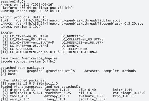
Therefore, it indeed follows that, when presented with 1 million ‘words’/digits of pi that are distributed with ‘no predictable biases’ over 1000 ‘corpus files’/bins, both measures should return values that are close to their theoretical minimums, which also means that the results Nelson reports would, if true, lead anyone to probably never consider DP_norm and D_KLnorm as measures of dispersion again. The main purpose of this correction is to demonstrate what the real results are and how that makes at least this part of Nelson’s argumentation collapse. To make my points as transparent and replicably as possible, this paper already contains the R code with which everyone can replicate the results for themselves – all one needs is an installation of R, the package magrittr, and internet access; readers can access a rendered Quarto document with all content, code, and my session info at <https://www.stgries.info/research/2024_STG_OnRNN_JQL.html>.

2. The overall distribution of the digits of Pi

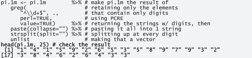
To demonstrate the falsity of both of Nelson’s results (and some additional small problems), let’s first download the first one million digits of pi, here from a website from the University of Exeter (output is shown in bold).

Given the way, pi is provided there, we need to prepare this a bit to get a vector of 1 million digits:

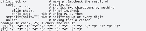
To make sure that these are the right numbers, let’s check these digits against those from another website.

There, too, we need a little bit of prep to get all the digits into a single vector:

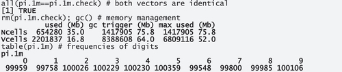
Crucially, both vectors contain the same digits so we can proceed with just pi.1 m for the rest of the paper; for one sanity check later, we also compute the frequencies of the digits.

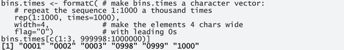
Nelson then ‘partitioned [this corpus] into 1,000 bins of 1,000 digits’ but does not say how so, for our replication, we will have to guess and explore the two most straightforward options. This is the first, which repeats the sequence of 1000 bin names 1000 times, and this is the second, which repeats the name of each of the 1000 bins 1000 times:

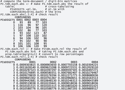
Many dispersion measures are straightforwardly computable from what, with regular corpora, would be term-document matrices and what, here, are digit-bin matrices. For each way of defining the bins, we compute one version with observed absolute frequencies and one with row proportions (because these latter ones will represent how much of each word as a proportion of all its uses is observed in each corpus bin).

For example, the 93/0.0009303815 in PI.tdm.each.abs‘s top left cell reflects that the 93 instances of’0’ in bin ‘0001’ corresponds to 0.0009303815 of the 99,959 instances of ‘0’ in the 1 m digits of pi.

For both dispersion measures, we then also need the expected, or prior, distribution. In this example, where we created the corpus files/bins as above, these are of course just one thousand instance of 0.001.

Nelson then shows the “noisy but unbiased dispersion of ‘7’ in pi in his Figure 2 (also p. 158). The right panel of his Figure 2 is fine and replicated here as Figure 1.

Figure 1. Nelson’s Figure 2 (right).

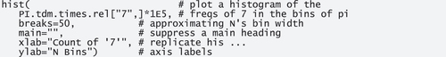
However, the left panel of his Figure 2 also seems wrong already. This is because its x-axis ranges from 1 to 1 million, presumably because the x-axis is the one million digits of pi, but it does so although – check the quote at the beginning of this paper – Nelson says ‘the numbers along the bottom show the position (in pi) of the part’ (my emphasis), meaning the x-axis should actually go from 1 to 1000. His x-axis labelling error seems confirmed by the fact that Nelson’s y-axis is labelled ‘Count of “7”’ and ranges from 0 to 140, suggesting that those are the frequencies of ‘7’ in every x-axis bin (as he described in the quote), and the vertical lines then shown in the plot seem to be the frequencies of 7 summarized in the histogram. But then that is why the current plot is wrong because one cannot have it both ways: only one of these two following plots would be correct:

• plot 1, where the x-axis goes from 1 to 1 m (for each word): This plot would be the kind of dispersion plot many apps provide, where each slot on the x-axis is for one word and each vertical line indicates whether the word in that corpus slot is a word in question (like, here, ‘7’). However, in such a plot, the y-axis would go from 0 (for FALSE, the digit is not ‘7’) to 1 (for TRUE, the digit is ‘7’), not from 0 to 140. Or,

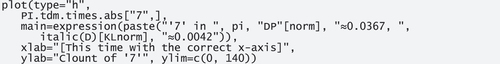
• plot 2, where the x-axis goes from 1 to 1000 (for each bin) and which, from his description, seems to be the intended one: There, this plot would indicate the frequency of ‘7’ in each bin and then, yes, the y-axis needs to go from 0 to 140. In my Figure 2, I am showing the plot he meant to show (but with a main heading I already changed to the averages of the results we will obtain below).

But his plot mixes up the axes: It has the x-axis from plot 1 and the y-axis from plot 2. Thus, it pretends that there are 1 million counts of ‘7’ between 80 and 140, i.e. around 100 million data points rather than the 1 million digits of pi he had us consider.

Figure 2. Nelson’s Figure 2 (left), one corrected version.

3. Computing DP_norm correctly

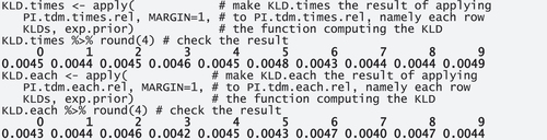
From the digit-bin matrices, we can compute the DP-values in a very R way: by applying to PI.tdm.times.rel (and PI.tdm.each.rel), namely each row/digit (MARGIN=1) an anonymous function, which will make the row an argument internally called obs.post (for ‘observed/posterior’) and then compute half of the sum of all absolute pairwise differences of obs.post and exp.prior, which is the formula for DP Nelson also provided:

These two sets of DP-values can then be normalized to the final DP_norm-values¹:

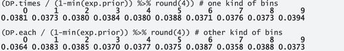
This is a result that makes a lot of sense given that, as per Nelson himself, ‘there are (famously) no predictable biases in the distribution of the digits of pi’ and the very low DP_norm values are perfectly compatible with that. However, it certainly is not the case that ‘every digit receives a DP_norm score 0.495 – nearly the midpoint of the range of the score’, that’s not even close to the truth. The DP_norm results he discusses on p. 158 and in Table 1 on p. 161 are wrong: The histogram in Figure 1 and the plot in Figure 2 are in fact perfectly compatible with a ‘value that might intuitively (and probably empirically) be interpreted as unbiased and even’.

4. Computing D_KLnorm correctly

First and for the record, Nelson makes another small mistake in his definition of D_KLnorm. On p. 155 of his article, he defines the Kullback-Leibler Divergence with his equation (4), which is shown here:

(1) $D_{\mathit{KLnorm}}=\mathit{D}\left(\mathit{O}||\mathit{E}\right)=\sum _{\mathit{i}=1}^N{O}_i\mathit{Lo}{g}_n\frac{O_i}{E_i}$(1)

To that, he adds ‘Where (as above) O is a vector of observed proportions and E is the vector of expected proportions’ (also p. 155). That is of course not correct because his equation 4 shown here in Equation (1)(1) $D_{\mathit{KLnorm}}=\mathit{D}\left(\mathit{O}||\mathit{E}\right)=\sum _{\mathit{i}=1}^N{O}_i\mathit{Lo}{g}_n\frac{O_i}{E_i}$(1) does not compute the normalized D_KL but a regular, unnormalized D_KL, something which Nelson implicitly admits in his very next sentence, where he says ‘InGries [sic] (2022), a normalization of this measure’s score, $D_{\mathit{KLnorm}}=1-e^{-\mathit{Dkl}}$, is proposed to fit the outputs to the unit interval’. In other words, his equation 4 is not already the normalized version, the normalized one we get only after also applying $D_{\mathit{KLnorm}}=1-e^{-\mathit{Dkl}}$.²

Let us now compute the D_KLnorm-values from the digit-bin matrices again. For that we first define a function that computes D_KL, which I here call KLDs; to try and replicate Nelson’s procedure, I am using the natural log in the function like he did. Then, we again apply this function to every row of PI.tdm.times.rel and PI.tdm.each.rel.

Any reader who does not trust my function can double-check the result for, say, ‘7’, with the following code (for PI.tdm.each.rel).

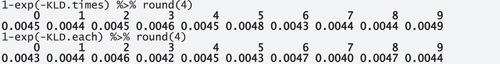
And then we normalize using the above-mentioned strategy.

As before with DP_norm, this result is exactly what one would expect D_KL or D_KLnorm to return for the digits of pi, what Nelson (2023, p. 158) himself formulated as an expectation, namely values that are close to 0 because that is the kind of ‘value that might intuitively (and probably empirically) be interpreted as unbiased and even’. But here the result is, in a sense, not even ‘only’ half off, this time Nelson’s results are at the exact opposite of the interval of values that D_KL can assume. He claims results of 0.9, but the real values are very close to 0.

5. Summary

In sum, Nelson (2023) commits six mistakes:

• the left panel of Figure 2 misrepresents the data studied;

• Equation (4) labels D_KL as D_KLnorm;

• the results reported for measuring the dispersion of the first 1 m digits of pi are false for

  • DP_norm (p. 158);

  • D_KLnorm (p. 158);

• the DP_norm results in Table 1 are false.

To reiterate: given the unpatterned first million digits of pi and contra Nelson, both DP_norm and D_KLnorm return exactly the results the measures are sensibly claimed to return: values close to 0 indicating even distributions/dispersions. This does of course not prove that either measure works perfectly for all realistic combinations of corpus sizes (in words and in parts) and word frequencies: we definitely need more studies that (i) explore how dispersion measures we already have ‘react’ to different scenarios, (ii) develop new measures and, importantly, (iii) validate them against other, external data (see, e.g. Biber et al., 2016; Burch et al., 2017, Gries 2022 for examples). Given the importance of dispersion as a corpus-linguistic quantity, it would certainly be great if corpus linguistics as a field devoted as much energy to dispersion measures as it has to association measures, but this of course requires that the computations are done correctly and replicably, which was the main point of this short note.

Disclosure statement

No potential conflict of interest was reported by the author(s).

Notes

1. In this very specific case, where all digit bins are equally large – ¹/₁₀₀₀ – the normalization formulae from Gries (2008) and Lijffijt and Gries (2012) amount to the same results; the R code I give here is the one that would work in the more general case where not all corpus files are equally large.

2. Also, the paper of mine he cites for D_KLnorm as a dispersion measure used the binary log, not the natural log Nelson’s equation uses.

References

- Biber, D., Reppen, R., Schnur, E., & Ghanem, R. (2016). On the (non)utility of Juilland’s D to measure lexical dispersion in large corpora. International Journal of Corpus Linguistics, 21(4), 439–464. https://doi.org/10.1075/ijcl.21.4.01bib
- Burch, B., Egbert, J., & Biber, D. (2017). Measuring and interpreting lexical dispersion in corpus linguistics. Journal of Research Design and Statistics in Linguistics and Communication Science, 3(2), 189–216. https://doi.org/10.1558/jrds.33066
- Gries, S. T. (2008). Dispersions and adjusted frequencies in corpora. International Journal of Corpus Linguistics, 13(4), 403–437. https://doi.org/10.1075/ijcl.13.4.02gri
- Gries, S. T. (2020). Analyzing dispersion. In M. Paquot & S. T. Gries (Eds.), A practical handbook of corpus linguistics (pp. 99–118). Springer.
- Gries, S. T. (2022). What do (most of) our dispersion measures measure (most) dispersion? Journal of Second Language Studies, 5(2), 171–205. https://doi.org/10.1075/jsls.21029.gri
- Lijffijt, J., & Gries, T. S. (2012). Correction to “dispersions and adjusted frequencies in corpora”. International Journal of Corpus Linguistics, 17(1), 147–149. https://doi.org/10.1075/ijcl.17.1.08lij
- Nelson, R. N. (2023). Too noisy at the bottom: Why Gries’ (2008, 2020) dispersion measures cannot identify unbiased distributions of words. Journal of Quantitative Linguistics, 30(2), 153–166. https://doi.org/10.1080/09296174.2023.2172711