An intelligent partial charging navigation strategy for electric vehicles

ABSTRACT

The rise of electric vehicles (EVs) has highlighted the issue of insufficient charging infrastructure, a major barrier to their widespread adoption. This problem is due to the limited capacity of existing charging networks and the performance constraints of EV batteries. Intelligent route planning, which optimizes travel time and energy use, could be a solution. Traditional studies on electric vehicle route planning oversimplify the charging process, assuming a linear relationship between charging level and time, neglecting its actual nonlinear nature. Additionally, these studies underestimate the impact of dynamically changing traffic conditions and charging station queue times on travel time. Integrating these factors into route planning can significantly reduce energy consumption and travel time. Our work proposes an intelligent partial charging strategy, relaxing full recharging restrictions, and fully considering the nonlinear battery characteristics, dynamic traffic conditions, and charging station queue times. Employing an improved genetic algorithm for route planning, our method demonstrates a dual advantage – reducing computational complexity and saving an average of 15% in travel time. Experimental results over a 400 km² traffic road network validate the efficiency of our approach, outperforming existing methods facing similar challenges.

KEYWORDS:

• Electric vehicles
• route planning
• partial charging
• genetic algorithm

1. Introduction

In recent years, with the growing concern over energy depletion and environmental problems worldwide, electric vehicles have become increasingly popular due to their green and energy-saving characteristics (Ullah, Zheng, et al. 2023). However, they have shorter cruising ranges and longer charging times compared to gasoline vehicles (Ullah, Safdar, et al. 2023). The public charging network for electric vehicles is small in scale, slow to grow, and unevenly distributed, which falls short of fully meeting the charging demand. This inadequacy leads to”range anxiety” (Hussain et al. 2022), where drivers constantly worry about running out of power while driving. Consequently, drivers tend to perform full recharges at charging stations, disregarding the nonlinear characteristics of the battery and potential traffic peaks. This often results in increased travel times and other associated problems.

It is difficult to solve problems from the origin, such as enhancing battery performance, optimizing charging network layout, and expanding the scale of the charging network (Ullah, Liu, Layeb, et al. 2023). In the real-world situation where the scale of the charging network remains unchanged and the performance of batteries cannot be readily improved, route planning may alleviate the problem as a soft way to save travel time, thus becoming a research hotspot. Previous studies have combined the Vehicle Routing Problem (VRP) with the new characteristics of electric vehicles such as battery capacity and charging station locations, thus reducing travel time to some extent. However, most of these works approximate the nonlinear charging characteristics as a linear process and assume full charge when vehicles visit charging stations (Andwari et al. 2017; Dimitrova and Maréchal 2017; Li et al. 2017; Montoya et al. 2016). Some studies use static traffic conditions and charging queue time for path planning, underestimating the impact of dynamically changing traffic conditions and charging queue time on travel time (Ullah, Liu, Yamamoto, et al. 2023). Fully incorporating the above factors into route planning may further save travel time. Therefore, this paper proposes an intelligent partial charging strategy that relaxes the Full Recharging (FR) restriction and realizes a corresponding route planning algorithm that fully considers the nonlinear characteristics of batteries, dynamic traffic conditions, and charging queue time at charging stations.

The rest of this paper is organized as follows: Section 2 reviews the related work. Section 3 defines the Constrained Shortest-path Problem for Electric Vehicles (CSP-EV), traffic road network and charging stations network model and gives the energy consumption function. Section 4 proposes an intelligent partial charging strategy and designs corresponding route planning algorithm. In Section 5, we analyze our proposed approach and evaluate the obtained results based on the experimental setup. Finally, we summarize the contributions of this paper and discuss the future work.

2. Related works

Existing works concerning CSP-EV can be categorized into two main types based on their purpose. The first type is primarily aimed at improving algorithm response speed and simplifying algorithm complexity (Goeke and Schneider 2015; Kchaou-Boujelben and Gicquel 2020; Soysal, Çimen, and Belbağ 2020), while the second type advances the first by aiming to find an energy or time optimal route. The most considered factors include traffic conditions, charging queue time, weather, etc (Froger et al. 2017; Gareau, Beaudry, and Makarenkov 2019; Storandt and Funke 2012; Zhong et al. 2022).

The first type of work views the problem as a Traveling Salesman Problem (TSP) and its derivatives, such as the constrained shortest-path problem for electric vehicles with charging (Goeke and Schneider 2015; Kchaou-Boujelben and Gicquel 2020; Soysal, Çimen, and Belbağ 2020), the constrained shortest-path problem for electric vehicles with time windows (Schneider, Stenger, and Goeke 2014; Xiao et al. 2019; Zuo et al. 2019), and the constrained shortest-path problem for electric vehicles with a mixed fleet (Cheng and Szeto 2017; Juan, Goentzel, and Bektaş 2014), among others. These studies consider additional features such as battery capacity and charging station locations on top of the traditional route planning algorithm and focus on reducing the complexity of the algorithm to obtain a feasible path more quickly.

Various studies of the second type have been conducted. Based on the Dijkstra algorithm, the potential shifting technique is used to solve the problem of negative edge costs (Storandt and Funke 2012; Zhong et al. 2022), accelerating the computation with Contraction Hierarchies. However, Storandt and Funke (2012) only considers the practical limitation of battery swapping stations in the real world. Zhong et al. (2022), on the other hand, additionally considers differences in user time utility, which means that the driving time and the dwell time at charging stations have different weights in the path planning process. However, it estimates traffic conditions and charging queue time through the Poisson process and queuing theory, respectively, which can only roughly approximate the actual conditions and may suffer from large errors. Gareau, Beaudry, and Makarenkov (2019) uses the improved K-shortest path algorithm to obtain multiple feasible paths by considering the charging queue time with a dynamic time graph re-labeling method. They simplified the charging process to a linear function of time and assumed full recharge. In practice, the approach proposed by Froger et al. (2017) assesses the importance of nonlinear charging functions and proposes a hybrid meta-heuristic. It concludes that the amount of charge is a key factor in path planning, and the better path should be based on piecewise or nonlinear charging functions.

The above works assumes full recharge and linearized charging process. Zhang et al. (2018) designs a simple partial charging strategy considering the non-linearity of the battery, the service frequency and service time of charging stations, improve the time query algorithm by Montoya et al. (2017) and obtain a shorter travel time. However, the partial charging strategy (Zhang et al. 2018) doesn’t consider dynamic changes in traffic conditions which may cause the vehicle meet congested traffic condition, and remains a sub-optimal solution. This paper proposes a more intelligent partial charging strategy that considers the traffic conditions and non-linear charging function, estimates traffic conditions and charging queue time through graph neural network models. We also design a novel encoding-and-decoding method to modify the genetic algorithm, lowering the computation complexity while solving for feasible paths with shorter travel time.

Overall, the contributions of our work are as follows:

1. An intelligent partial charging navigation strategy for electric vehicles.

2. A partial charging strategy considering dynamic traffic conditions and non-linear charging function, which can trade-off charging amount and travel time.

3. A priority-based dynamic coding and decoding method to make the genetic algorithm more adaptable to CSP-EV.

3. Problem statement and theoretical model

3.1. Constrained shortest-path problem for electric vehicle(CSP-EV)

Formulate the CSP-EV model based on the notations listed below:

• $\mathit{V}$ =$\{\mathit{v}|\mathit{v}=1,2,\dots ,\mathit{n}\}$ is the set of nodes including road intersections and charging stations.

• $w_e(v_i,v_{\mathit{i}+1})$ represents the driving time from vertex $v_i$ to vertex $v_{\mathit{i}+1}$.

• $\mathit{P}$ =$\{v_i|\mathit{i}=1,2,\dots ,\mathit{k}\}$ is the set of travel nodes.

• $v_r$: Selected charging station.

• $\mathit{ct}(v_r)$): Charging time at charging station vr.

• $\mathit{wt}(v_r)$: Waiting time at charging station vr.

• $b_0$: Initial SoC(State of Charge).

• $\mathit{b}$: Real-time SoC.

• $\mathit{M}$: Maximum SoC.

• $\mathit{bc}(\mathit{e})$: Energy consumption of road e.

• $\mathit{cm}$: Charging amount at charging station $v_r$.

• $\mathit{tt}$: Total travel time.

With the above given symbols, CSP-EV can be defined as the problem of finding the optimal travel route, including charging stations, from the starting point to the destination, while satisfying the electricity constraints given by Equation (2)(2) $\left\{\begin{array}{c}0<\mathit{b}\le \mathit{M}\\ \mathit{b}(v_{\mathit{i}+1})=\mathit{b}(v_i)-\mathit{bc}(e_{\mathit{i},\mathit{i}+1}),\mathit{i}<\mathit{n}-1\mathit{and}{v}_{\mathit{i}+1}\ne v_r\\ \mathit{b}(v_{\mathit{i}+1})=\mathit{b}(v_i)+\mathit{cm},v_{\mathit{i}+1}=v_r\end{array}\right.$(2) , so as to minimize the objective function represented by Equation (1)(1) $\mathit{t}\mathit{t}=min\sum _{\mathit{i}=1}^{\mathit{k}-1}{w}_e(v_i,v_{\mathit{i}+1})+\mathit{ct}(v_r)+\mathit{wt}(v_r)$(1) .

(1) $\mathit{t}\mathit{t}=min\sum _{\mathit{i}=1}^{\mathit{k}-1}{w}_e(v_i,v_{\mathit{i}+1})+\mathit{ct}(v_r)+\mathit{wt}(v_r)$(1)

(2) $\left\{\begin{array}{c}0<\mathit{b}\le \mathit{M}\\ \mathit{b}(v_{\mathit{i}+1})=\mathit{b}(v_i)-\mathit{bc}(e_{\mathit{i},\mathit{i}+1}),\mathit{i}<\mathit{n}-1\mathit{and}{v}_{\mathit{i}+1}\ne v_r\\ \mathit{b}(v_{\mathit{i}+1})=\mathit{b}(v_i)+\mathit{cm},v_{\mathit{i}+1}=v_r\end{array}\right.$(2)

Equation (1)(1) $\mathit{t}\mathit{t}=min\sum _{\mathit{i}=1}^{\mathit{k}-1}{w}_e(v_i,v_{\mathit{i}+1})+\mathit{ct}(v_r)+\mathit{wt}(v_r)$(1) aims to get the minimum travel time including the travel time, charging queue time and charging time. The first equation in Equation (2)(2) $\left\{\begin{array}{c}0<\mathit{b}\le \mathit{M}\\ \mathit{b}(v_{\mathit{i}+1})=\mathit{b}(v_i)-\mathit{bc}(e_{\mathit{i},\mathit{i}+1}),\mathit{i}<\mathit{n}-1\mathit{and}{v}_{\mathit{i}+1}\ne v_r\\ \mathit{b}(v_{\mathit{i}+1})=\mathit{b}(v_i)+\mathit{cm},v_{\mathit{i}+1}=v_r\end{array}\right.$(2) illustrates the battery capacity limitation during the electric vehicle’s journey, it should be greater than 0 and less than the maximum capacity, M. The second and third equations describe the method of updating the battery capacity during the journey.

3.2. Traffic conditions and charging queue time prediction model

In order to save travel time, we need to choose unblocked roads, charging stations with short queue time and appropriate amount of charging, all of which need to predict traffic conditions and charging queue time. The traffic road network and charging stations network can be described by a unified model:

(3) $\left\{\begin{array}{c}{G}^{\mathrm{T}}=(\mathit{V},\mathit{E},\mathit{W})\\ \mathit{V}=\left\{\mathit{v}|\mathit{v}=1,2,\dots ,\mathit{n}\right\}\\ \mathit{E}=\left\{e_{\mathit{ij}}|\mathit{i}\ne \mathit{j}\right\}\\ \mathit{W}=\left\{w_{\mathit{ij}}|e_{\mathit{ij}}\in \mathit{E}\right\}\end{array}\right.$(3)

(4) $w_{\mathit{ij}}=\left\{\begin{array}{c}{w}_{\mathit{ij}},{\mathrm{e}}_{\mathit{ij}}\in \mathit{E}\\ 0,{\mathrm{v}}_i=v_j\\ \mathrm{\infty },{\mathrm{e}}_{\mathit{ij}}\notin \mathit{E}\end{array}\right.$(4)

For traffic road network: $\mathit{G}$ represents the traffic road network; $\mathit{V}$ is the set of all nodes in the graph, including road intersections and charging stations; $\mathit{E}$ is the set of road sections between two nodes; $\mathit{W}\in$ $R^{\mathit{N}\times \mathit{N}}$ represents the average travel time of each road which can be represented by the graph signal $\mathit{X}(\mathit{t})\in$ $R^{\mathit{N}\times 1}$.

For charging stations network: $\mathit{G}$ represents the charging stations network; $\mathit{V}$ is the set of charging stations; $\mathit{E}$ is the set of connections between two stations; $\mathit{W}\in$ $R^{\mathit{N}\times 1}$ is the weighted adjacency matrix, representing the degree of node correlation. At this time, the graph signal $\mathit{X}(\mathit{t})$ observed on $\mathit{G}$ represents the charging queue time of charging stations collected at time $\mathit{t}$;

Given the network $\mathit{G}$ and corresponding graph signal $\mathit{X}$, the prediction can be seen as a function $\mathit{h}(.)$, which maps the historical graph signal of $\mathit{T}{ }^{\mathrm{\prime }}$-length time period to the graph signal of future $\mathit{T}$-length time period. That is, given a digraph $\mathit{G}$, the prediction problem is expressed as:

(5) $\left[\mathit{X}\left(\mathit{t}-T^{\prime }+1\right),\dots ,\mathit{X}(\mathit{t});\mathit{G}\right]\stackrel{\mathit{h}(\cdot )}{\to }[\mathit{X}(\mathit{t}+1),\dots ,\mathit{X}(\mathit{t}+\mathit{T})]$(5)

So we need to learn $\mathit{h}(\cdot )$ to predict traffic conditions and charging queue time. But this kind of prediction always suffers high-level data noise, complex features, complex space-time correlation and heterogeneity, which makes it difficult to establish effective models. And with the development of the Internet of Things, the data scale is getting larger (Li et al. 2016) which makes it even more difficult to mine and learn the temporal relations. At present, the prediction model based on graph neural network has achieved promising results and become the mainstream method (Xiao, Guo, et al. 2023; Xiao, Wu, et al. 2023). Therefore, this paper uses the Diffusion Convolutional Recurrent Neural Network (DCRNN) (Li et al. 2017) and the Spatial-Temporal Synchronous Graph Convolutional Network (STSGCN) (Song et al. 2020) establish the traffic condition prediction model and the charging queue time prediction model.

3.3. Energy consumption function

To ensure that power do not run out midway, it is important to accurately calculate real-time power during path planning, so we need a precise energy consumption function. In relevant research, the energy consumption value of 100 $\mathit{km}$ is generally taken as the measurement standard. Xiao et al. (2021) divides electric vehicle energy consumption into five components: aerodynamic loss, tire loss, power train loss, auxiliary loss and kinetic/potential energy loss. The paper accurately fits the energy consumption curve through experiments. To facilitate the calculation of the routing problem, the formulas have been simplified, resulting in an energy consumption formula that depends only on the driving speed and load. Since our research primarily focuses on the routing algorithm itself, and the accuracy of this formula surpasses other baseline methods, we adopt this formula for energy consumption calculations in this study. The energy consumption function of each part is shown in Equation (6)(6) $\left\{\begin{array}{c}\begin{array}{c}\mathit{EC}{R}_{\mathit{air}}=\frac{1}{2}\mathit{\rho ACd}{v}^2\mathit{d}\times \frac{1000}{3600},\\ \mathit{EC}{R}_{\mathit{tire}}=\left(\mathit{W}+\mathit{f}\right)\mathit{g}{C}_r\mathit{cos}(\mathit{\varphi })\mathit{d},\\ \mathit{EC}{R}_{\mathit{Dr}}=({\alpha }_{\mathit{Dr}}{v}^3+{\beta }_{\mathit{Dr}}{v}^2+{\gamma }_{\mathit{Dr}}\mathit{v}+C_{\mathit{Dr}})\mathit{d}/\mathit{v},\\ \mathit{EC}{R}_{\mathit{ancillary}}=\left(P_{\mathit{A}/C}+P_{\mathit{others}}\right)\mathit{d}/\mathit{v},\\ \mathit{EC}{R}_{\mathit{kp}}=\left(\mathit{W}+\mathit{f}\right)[\mathit{gsin}(\mathit{\varphi })\mathit{d}+\mathit{a}].\end{array}\end{array}\right.$(6) :

(6) $\left\{\begin{array}{c}\begin{array}{c}\mathit{EC}{R}_{\mathit{air}}=\frac{1}{2}\mathit{\rho ACd}{v}^2\mathit{d}\times \frac{1000}{3600},\\ \mathit{EC}{R}_{\mathit{tire}}=\left(\mathit{W}+\mathit{f}\right)\mathit{g}{C}_r\mathit{cos}(\mathit{\varphi })\mathit{d},\\ \mathit{EC}{R}_{\mathit{Dr}}=({\alpha }_{\mathit{Dr}}{v}^3+{\beta }_{\mathit{Dr}}{v}^2+{\gamma }_{\mathit{Dr}}\mathit{v}+C_{\mathit{Dr}})\mathit{d}/\mathit{v},\\ \mathit{EC}{R}_{\mathit{ancillary}}=\left(P_{\mathit{A}/C}+P_{\mathit{others}}\right)\mathit{d}/\mathit{v},\\ \mathit{EC}{R}_{\mathit{kp}}=\left(\mathit{W}+\mathit{f}\right)[\mathit{gsin}(\mathit{\varphi })\mathit{d}+\mathit{a}].\end{array}\end{array}\right.$(6)

The total energy consumption function is shown in Equation (7)(7) $\mathit{ECR}=\mathit{EC}{R}_{\mathit{air}}+\mathit{EC}{R}_{\mathit{tire}}+\mathit{EC}{R}_{\mathit{drv}}+\mathit{EC}{R}_{\mathit{anc}}+\mathit{EC}{R}_{\mathit{kp}}$(7) and the meaning of related notations are shown in Table 1.

(7) $\mathit{ECR}=\mathit{EC}{R}_{\mathit{air}}+\mathit{EC}{R}_{\mathit{tire}}+\mathit{EC}{R}_{\mathit{drv}}+\mathit{EC}{R}_{\mathit{anc}}+\mathit{EC}{R}_{\mathit{kp}}$(7)

Table 1. Notation for description of energy consumption function.

Symbol	Actual meaning
$\mathit{ECR}$	Energy consumption rate (W-h/km)
$\mathit{A}$	Vehicle frontal area (${\mathrm{m}}^2$)
$\mathit{\rho }$	Air density (kg/${\mathrm{m}}^3$)
$C_d$	Air drag coefficient
$\mathit{\upsilon }$	Speed (m/s)
$\mathit{d}$	Travel distance (m)
$\mathit{W}$	Mass (kg)
$\mathit{f}$	Load (kg)
$\mathit{g}$	Gravitational acceleration
$C_r$	Rolling friction coefficient
$\mathit{\varphi }$	Road angle(°)
${\alpha }_{\mathit{Dr}}$ ${\beta }_{\mathit{Dr}}$ ${\gamma }_{\mathit{Dr}}$	Constant coefficient related to vehicle type
$C_{\mathit{Dr}}$	Power consumption of transmission system
	When the vehicle is stationary
$P_{\mathit{A}/C}$	Power of air conditioning system (W)
$P_{\mathit{others}}$	Other auxiliary power system power (W)

The calculation of energy consumption can be simplified into an version with load and driving speed as variables, so the key of energy consumption calculation relies on accurate driving speed estimation.

4. The basic approach

4.1. Partial charging strategy design

Partial charging strategy means deciding the charging amount that minimizes travel time on the basis of ensuring the minimum SoC (supporting the vehicle to go to the nearest charging station from the terminal) at the end point. It is mainly affected by non-linear characteristics of the battery and subsequent changes of traffic conditions. We will then give examples and discuss the influence deeply.

(1) Influence of traffic conditions on charging amount selection.

Traffic conditions are highly volatile over time, and a smooth road can become extremely congested for a short period of time (Keler, Krisp, and Ding 2017). Sometimes charging for a little longer may meet the subsequent peak traffic conditions, making the travel time increase significantly.

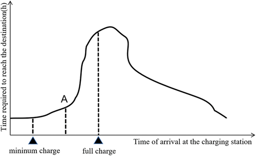
For example, as shown in Figure 1, A is the dividing point between smooth and congestion traffic conditions. After charging to the minimum required charge, we can charge to point A at most. If we default to full recharge, the travel time will increase significantly. When we leave between the minimum required charge and point A, we can save travel time while obtaining enough SoC.

Figure 1. Example of traffic conditions becoming congested after reaching charging station.

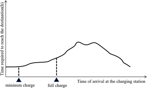
As the example shown in Figure 2, there is no significant change in traffic conditions after reaching the charging station. We can choose charging amount according to our personal needs, either full recharge or just enough, which can avoid wasting time in meaningless road congestion.

Figure 2. Example of traffic conditions remaining unchanged after reaching charging station.

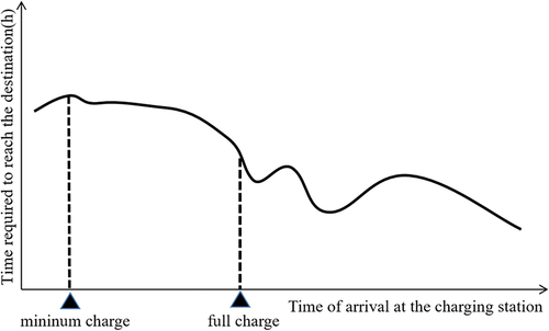
As the example shown in Figure 3, the traffic conditions gradually clear up after reaching the charging station. We can instead choose charge more to avoid the peak traffic conditions and exchange the meaningless traffic jam time for more electricity.

Figure 3. Example of traffic conditions becoming smooth after reaching charging station.

Therefore, when performing route planning, we need to accurately predict the traffic conditions, which can not only help us avoid congested roads and save driving time, but also help us to reasonably balance the choice of charging amount. If the subsequent traffic conditions become congested, we can choose to charge the vehicle to the minimum required power; If there is no significant change or become smooth, we can choose full recharge. By doing so, we can save travel time with a certain amount of power remaining.

(2) The influence of battery nonlinear characteristics on charging amount selection.

To safeguard the charging battery from potential damage, the charging speed is adjusted as the battery approaches full capacity (Ullah et al. 2022; Ullah, Liu, Yamamoto, Shafiullah, et al. 2023). Specifically, a slower charging speed is implemented for batteries with relatively higher State of Charge (SoC) levels. The recharging process follows a linear pattern until the battery reaches 80% charge. Beyond this critical percentage, the amperage is gradually reduced to mitigate potential damage to the battery. In this study, we employ a linear regression to model the charging process up to 80% battery level. Subsequently, we utilize a quadratic polynomial equation to characterize the battery charging curve from 80% to full capacity (Figure 4).

Figure 4. Piecewise approximation of charging curve.

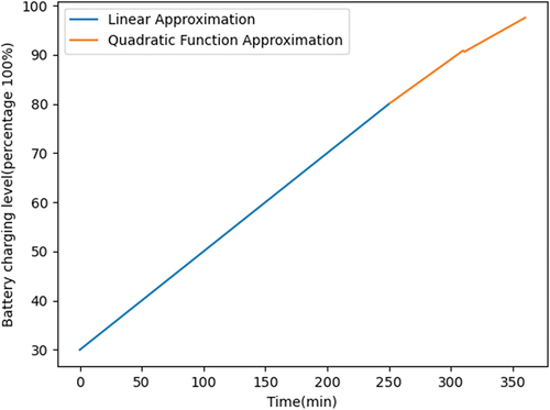
The influence of the battery non-linear characteristics on the selection of the charging amount is mainly reflected in the charging speed getting slower and slower as the power increases, so we should avoid full recharge as much as possible. The time required to charge to the minimum reserved charge is much less than the time required to full charge. Travel time is gradually wasted in the charging process, the benefits from increased electricity are offset. This brings us two inspirations. First, we can use the SoC on arrival as one of the criteria to choose the charging station. The less the SoC, the higher the charging efficiency, thus saving the total travel time. Second, we need to balance the positive benefits of increased charging amount with the negative benefits of a non-linear increase in travel time and make a trade-off between charging amount and travel time.

4.2. Charging navigation based on genetic algorithm

Following our discussion, the algorithmic level necessitates the selection of the travel path, charging station, and charging amount. Genetic algorithms are widely used in path planning problems due to its generality and parallelism. Natural organisms evolve by recombination and mutation of genes in the cycle of reproduction, so that they constantly have new traits to adapt to the complex and changing environment. The genetic algorithm streamlines this complex genetic process and abstracts a set of mathematical models to represent complex phenomena in a simpler encoding, and achieves a heuristic search of the complex search space, which can eventually find the global optimal solution with a large probability, while inherently supporting parallel computing.

Encoding and decoding are important steps of genetic algorithm, which can be regarded as the mutual mapping process of solutions in the solution space and gene arrangement inside the chromosome. The previous encoding methods include binary encoding, floating point encoding and symbolic encoding, which have the following problems for CSP-EV in this paper:

1. Previous algorithms used binary encoding method, where each road was considered as a single binary code, with 0/1 representing not passing through/through the road. This approach can represent the passing roads intuitively, but cannot ensure a connected solution and requires adding some constraints during the search process, which reduces the search speed and accuracy.

2. The previous encoding method cannot represent the path including charging station and charging amount at the same time. During the search process, the charging station may appear at any location of the solution, and the charging amount is an arbitrary floating point number between 0 and 100, which is difficult to represent in a binary way as the path search.

3. The previous decoding method cannot distinguish between road nodes and charging stations, and cannot update the real-time power. It’s also inefficient and slow in search because the calculation of the objective function needs to be based on dynamic traffic conditions and charging queuing time which has a high degree of complexity.

To solve the above problems, we design a priority based dynamic encoding and decoding method. It is assumed that there are $\mathit{n}$ +1 genes on the chromosome with hybrid coding scheme. The first $\mathit{n}$ genes with permutation coding (random non-repeated permutation of n numbers in 1$\sim$ $\mathit{n}$) represent the priority of n nodes including charging stations, the ($\mathit{n}$ +1)$\mathrm{th}$ bit is encoded as a floating point number, which represents the charging amount. We also need a set $\mathit{C}$ to store the connected nodes of each node, which is convenient to decode the connected path. We will give an simple example of how this approach works. Figure 5 shows a simple road network, where node 2 and node 6 represent charging stations. The corresponding node connection set $\mathit{C}$ is [[2, 3], [3, 4, 5], [5, 6], [7, 8], [4, 6], [7, 9], [8, 9], [9, 10], [10]]. Table 2 shows an example of chromosome.

Figure 5. Schematic diagram of a simple road network.

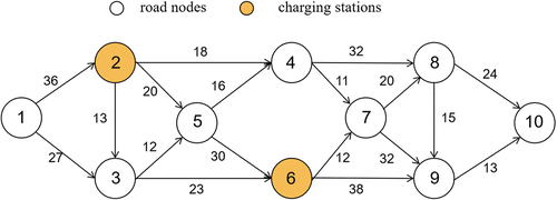
Table 2. Example of chromosome structure.

Node number	1	2	3	4	5	6	7	8	9	10	11
Priority	7	3	4	6	2	5	8	10	1	9	11

Suppose we go to node 10 from node 1, the corresponding element of node 1 in set $\mathit{C}$ is [2, 3], indicating that we can go to node 2 or 3 next. The corresponding priorities of the two nodes in the chromosome are 3 and 4, so we select node 4 with higher priority. And so on, until we reach node 10.

During the execution of the genetic algorithm, we need to update real-time SoC. When going to a new node, subtract the corresponding power consumption. When reaching a charging station, update to the SoC indicated by the ${11}^{\mathit{th}}$ element of chromosome. Then we calculate the population fitness based on the decoded paths, dynamic traffic conditions and charging queuing time. Then we calculate the population fitness based on the decoded paths, dynamic traffic conditions and charging queue time. To ensure the power constraint is satisfied, we set a penalty function with real-time power as input to reduce the fitness of solutions that do not satisfy the constraint.

We also introduce a real-coded crossover operator based on the Laplace distribution to expedite the algorithm’s convergence rate. This operator centers on the parent solutions, and the probability density function of the Laplace distribution is as follows:

(8) $\mathit{f}(\mathit{x})=\frac{1}{2\mathit{b}}exp\left(-\frac{|x-a|}{b}\right),-\mathrm{\infty }<\mathit{x}<\mathrm{\infty }$(8)

$\mathit{a}\in$ R is known as the location parameter, and $\mathit{b}$$>$0 is the scale parameter. The probability density function of the Laplace distribution is given by:

(9) $\mathit{F}(\mathit{x})=\left(\begin{array}{cc}\frac{1}{2}exp\left(\frac{|x-a|}{b}\right),& \mathit{x}\le \mathit{a},\\ 1-\frac{1}{2}exp\left(-\frac{|x-a|}{b}\right),& \mathit{x}>\mathit{a},\end{array}\right.$(9)

Assuming two parents denoted as $\mathit{x}(1)$ and $\mathit{x}(2)$, and two offspring as $\mathit{y}(1)$ and $\mathit{y}(2)$. A uniformly distributed random number $\mathit{u}\in$[0,1] is first generated. Following this, by inverting the cumulative distribution function of the Laplace distribution as follows, a random number $\mathit{\beta }$ is derived. This number follows the Laplace distribution.

(10) $\mathit{\beta }=\left\{\begin{array}{cc}\mathit{a}-\mathit{b}{log}_e(\mathit{u}),& \mathit{u}\le \frac{1}{2}\\ \mathit{a}+\mathit{b}{log}_e(\mathit{u}),& \mathit{u}>\frac{1}{2}.\end{array}\right.$(10)

The two offspring are represented as:

(11) $\left\{\begin{array}{c}{y}_i^{(1)}=x_i^{(1)}+\mathit{\beta }\\ y_i^{(2)}=x_i^{(2)}+\mathit{\beta }\end{array}\left|\begin{array}{c}{x}_i^{(1)}-x_i^{(2)}\\ x_i^{(1)}-x_i^{(2)}\end{array}\right|\begin{array}{c},\\ .\end{array}\right.$(11)

The positions of these two offspring are symmetrically placed relative to their parents. For smaller values of $\mathit{b}$, the offspring are likely to be generated near the parents, while for larger values of $\mathit{b}$, the offspring are expected to be generated far from the parents. For fixed values of $\mathit{a}$ and $\mathit{b}$, if the parents are close to each other, the offspring will also be close to each other. Conversely, if the parents are far apart, the offspring are likely to be distant from each other. The algorithm is shown in Figure 6.

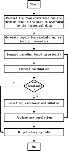
Figure 6. Charging navigation flow chart.

5. Experimental analysis

5.1. Example setup

In order to test the actual effect of the proposed method, we constructed a 20 km × 20 km road network containing 31 nodes and set up four charging stations with reference to the distribution characteristics of charging piles in Shanghai, as shown in Figure 7. The road section weights in the figure indicate the actual distance (unit: km), the dashed circles represent charging stations, and the attributes of each charging station are shown in Table 3. In addition, we choose Tesla Model3 as the test vehicle to establish the energy consumption model, and the relevant parameters are shown in Table 4. Inserting the parameters from the table into Equation (6)(6) $\left\{\begin{array}{c}\begin{array}{c}\mathit{EC}{R}_{\mathit{air}}=\frac{1}{2}\mathit{\rho ACd}{v}^2\mathit{d}\times \frac{1000}{3600},\\ \mathit{EC}{R}_{\mathit{tire}}=\left(\mathit{W}+\mathit{f}\right)\mathit{g}{C}_r\mathit{cos}(\mathit{\varphi })\mathit{d},\\ \mathit{EC}{R}_{\mathit{Dr}}=({\alpha }_{\mathit{Dr}}{v}^3+{\beta }_{\mathit{Dr}}{v}^2+{\gamma }_{\mathit{Dr}}\mathit{v}+C_{\mathit{Dr}})\mathit{d}/\mathit{v},\\ \mathit{EC}{R}_{\mathit{ancillary}}=\left(P_{\mathit{A}/C}+P_{\mathit{others}}\right)\mathit{d}/\mathit{v},\\ \mathit{EC}{R}_{\mathit{kp}}=\left(\mathit{W}+\mathit{f}\right)[\mathit{gsin}(\mathit{\varphi })\mathit{d}+\mathit{a}].\end{array}\end{array}\right.$(6) , with the load $\mathit{f}$ set to 100 kg.

Figure 7. Schematic diagram of road network structure.

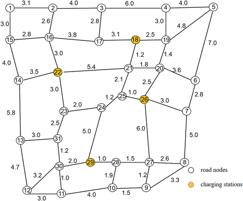
Table 3. Charging station properties.

Charging station	Corresponding node	Arrival intensity	Service intensity	Number of charging piles
1	18	8	4	4
2	22	4	4	8
3	26	3	4	6
4	29	10	4	4

Table 4. Parameters of Tesla Mode3.

Parameters	Value
Long × wide × high(mm)	4694 × 1850 × 1443
Curb weight(kg)	1761
Wheelbase(mm)	2857
Battery energy(kWh)	78.4
{power consumption(kWh/100km)	13.2
Range(km)	675

5.2. Analysis of partial charging strategy

To evaluate if a partial charging strategy can effectively balance the charging quantity and travel time, thereby minimizing travel time while maintaining the minimum required power, we assume a scenario where a vehicle traverses from node 1 to node 8, ensuring a minimum of 35% of full charge capacity is retained. Meanwhile, in order to show the completeness of the experiment, we conducted 100 experiments with initial SoC from 1% to 100% in three cases: random traffic condition, traffic condition becomes congested, and traffic condition becomes smooth, respectively, and recorded the changes of travel time and remaining power. The experimental results are shown in Figure 8.

Figure 8. Changes in travel time and remaining SoC.

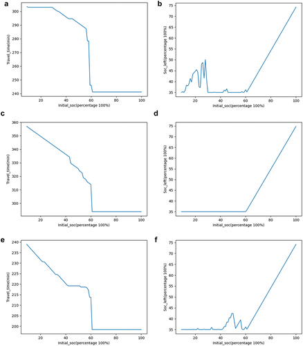
We can find the trend of travel time is approximately the same in all three cases. The travel time remains the same when the initial SoC is between 61% and 100%, indicating that no charging is needed at this time and the same path is chosen. It has a jump when the initial SoC is 60%, because the electric vehicle needs to recharge, so the charging queue time and charging time need to be added to travel time. When the initial SoC is between 60% and 9%, the travel time increase non-linearly because of the increasing queue time and nonlinear charging characteristics. When the initial SoC is less than 9%, the electric vehicle cannot reach the end point because its initial SoC cannot support it to the nearest charging station.

In all three conditions, the remaining SoC has the same trend when the initial SoC is between 61% and 100%, but has different trend when initial SoC is between 9% and 60%. As shown in Figure 8(b), when the traffic conditions get worse, the partial charging strategy chooses to charge just enough to save travel time, thus always keeping a 35% remaining SoC. In Figure 8(d), when the traffic conditions become better, the partial charging strategy determines the charging amount based on the positive effect of subsequent better traffic conditions versus the negative effect of the nonlinear charging characteristics, so the remaining SoC is not always 35%. The remaining power variation shown in Figure 8(f) combines both two cases. In addition, by looking at the selected paths, we can find that the paths selected at initial SoC of 39% and 25% are both 1 → 2 → 3 → 17 → 18 → 21 → 25 → 26 → 27 → 8, but the former chooses charging station 26 while the later chooses 18. Components of travel time are shown in Table 5. This is because of the influence of non-linear charging characteristics. During path planning, there is a tendency to select charging stations closer to the destination, optimizing for a lower battery level upon reaching the station, leading to faster charging and ultimately saving travel time. Therefore, with an initial battery level of 39%, charging is done at station 26 to minimize total travel time (203.0 min if charging at station 18). In contrast, with an initial battery level of 25%, reaching station 26 is not feasible, and charging at station 18 becomes the only option.

Table 5. Components of travel time.

Initial SOC	Driving time(min)	Waiting time(min)	Charging time(min)	Charging station	Total time(min)
39%	176.0	5.0	10.0	26	191.0
25%	178.9	5.0	28.0	18	211.9

5.3. Analysis of dynamic traffic condition

To validate the potential further reduction in total travel time considering future changes in traffic conditions, under the premise of random variations in traffic, we conducted simulations with the same settings as described in Section 5.2. We compared the total travel time when considering and not considering changes in traffic conditions. The final results are shown in Figure 9, confirming that considering future changes in traffic conditions indeed contributes to saving travel time.

Figure 9. Travel time curve with dynamic and static traffic condition.

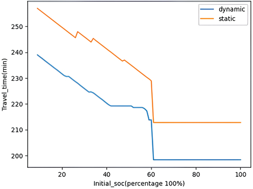
Analyzing two scenarios with initial battery levels of 100% and 10%, when the initial battery level is 100%, the path chosen based on dynamic traffic conditions is 1→2→3→4→19→20→6→7→8, resulting in a total travel time of 175.2 min. In contrast, the path chosen based on static traffic conditions is 1→2→16→22→21→20→26→7→8, with a travel time of 227.6 min. When the initial battery level is 10%, the path chosen based on dynamic traffic conditions is 1→2→3→17→18→21→25→26→27→8, with a remaining battery level of 35.1%. The routes in both cases are shown in the Figure 10. Charging occurs at the station at node 18 during the journey, resulting in a total travel time of 199.8 min. The path chosen based on static traffic conditions is 1→2→3→17→18→21→20→26→7→8, with a remaining battery level of 35%, and charging at the station at node 18 during the journey, resulting in a total travel time of 227.3 min. The distribution of total travel time is shown in Table 6, revealing that considering future changes in traffic conditions allows for avoiding congested roads and effectively reducing travel time.

Figure 10. Planned routes under different traffic condition characteristics.

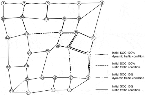
Table 6. Comparison of results considering traffic condition changes.

Initial SOC	Traffic attributes	Driving time(min)	Waiting time(min)	Charging time(min)	Travel time(min)
100%	Dynamic	175.2	–	–	175.2
	Static	227.6	–	–	227.6
10%	Dynamic	178.9	5.0	28.0	211.9
	Static	204.3	15.0	36.5	255.8

5.4. Algorithm analysis and comparison

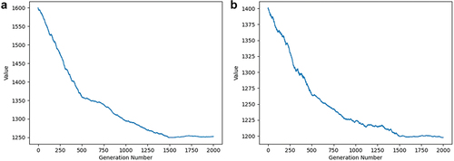
Firstly, we verify the convergence of the algorithm by recording the changes in the objective function value within 2000 generations under two different initial battery levels: 100% and 28%. The convergence graph are shown in Figure 11, it can be observed that the algorithm quickly converges to a stable value.

Figure 11. Convergence graph of genetic algorithm.

In order to test the effect of our algorithm, we take the running time and travel time as evaluation indicators to compare with three algorithms: the traditional genetic algorithm, the improved time optimization algorithm (Zhang et al. 2018) and Two-Layer genetic algorithm (Karakatič 2021). Randomly conduct eight queries, the results are shown in Figures 12 and 13.

Figure 12. The comparison of running time.

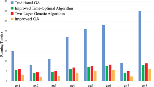
Figure 13. The comparison of travel time.

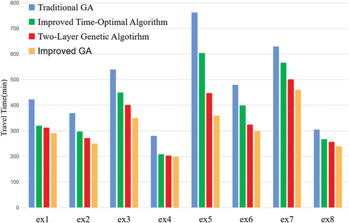
We have achieved significant optimization in the running time of our algorithm compared to the other three methods. This is primarily due to the implementation of a priority-based dynamic encoding and decoding genetic algorithm, which allows us to pre-screen infeasible routes and greatly enhances the overall running efficiency. Additionally, by harnessing the parallelism capabilities of the genetic algorithm, we are able to further reduce the execution time.

In all eight examples, our algorithm consistently demonstrates shorter travel times compared to the other algorithms. While the two-layer genetic algorithm only accounts for the battery’s nonlinear charging characteristics, the improved time optimization algorithm takes into consideration the battery’s nonlinear characteristics to devise a simple partial charging strategy. This strategy involves traveling to the furthest charging station within the current range and charging the battery to a level sufficient to reach either the destination or the next farthest practical charging station. However, the partial charging strategy presented in this paper is more comprehensive as it factors in dynamic traffic conditions and nonlinear charging characteristics. Additionally, the route planning in this study is based on dynamic traffic conditions and charging queue time, resulting in reduced driving and waiting times.

6. Conclusion and future work

The burgeoning proliferation of electric vehicles in urban environments has spurred our investigation into associated route planning algorithms that alleviate commuting stress. This paper takes into account traffic conditions, charging queue durations, and nonlinear charging dynamics in a comprehensive manner. We propose an intelligent partial charging strategy and develop a route planning algorithm with the purpose of minimizing travel time. Meanwhile, to reduce the complexity of the genetic algorithm, we design a priority-based dynamic encoding and decoding approach as well as dynamic variation rate and cross rate selection functions. Experiments show that our algorithm makes a significant improvement in travel time and algorithm complexity. Our partial charging strategy can balance the charging amount and travel time, saving travel time while ensuring the minimum remaining power.

This paper assumes that we can only go to the charging station once in a single trip. We will continue to study the problem that electric vehicles can be recharged multiple times on a long trip. At the same time, improving the execution speed of algorithms in large-scale road networks is also a major research issue for the future.

Disclosure statement

No potential conflict of interest was reported by the author(s).

Data availability statement

The data that support the findings of this study are available from the corresponding author, [[email protected]], upon reasonable request.

Additional information

Funding

This research was supported by the National Key Research and Development Program [grant number 2021YFB2501104].

Notes on contributors

Jinsheng Xiao

Jinsheng Xiao is an associate professor of Information and Communication Engineering with the Electronic Information School, Wuhan University. He received the PhD degree in mathematics from Wuhan University. His research interests are image and video processing and computer vision.

Bang Sun

Bang Sun received a BE degree from Wuhan University. His research interests include big data analytic and smart transportation.

Xun Gao

Xun Gao is a professor of Information and Communication Engineering with the Electronic Information School, Wuhan University. His research interests are Information processing and Communication.

Hua Yang

Hua Yang was born in 1974. He received his PhD degree in computer software theory from Wuhan University, China, in 2009. He worked at Wuhan University until 2015 and is currently a professor at Guizhou Normal University. From 2015 to 2016, he was an academic visitor at the University of Nottingham, UK. His research interests include data mining, machine learning, and natural language processing.

Liyuan Wang

Liyuan Wang is a senior engineer in the field of intelligent transportation.

References

- Andwari, A., A. Pesiridis, S. Rajoo, R. Martinez-Botas, and V. Esfahanian. 2017. “A Review of Battery Electric Vehicle Technology and Readiness Levels.” Renewable and Sustainable Energy Reviews 78: 414–430. https://doi.org/10.1016/j.rser.2017.03.138.
- Cheng, Y., and W. Szeto. 2017. “Artificial Bee Colony Approach to Solving the Electric Vehicle Routing Problem.” Journal of the Eastern Asia Society for Transportation Studies 12: 975–990. https://doi.org/10.11175/easts.12.975.
- Dimitrova, Z., and F. Maréchal. 2017. “Environomic Design for Electric Vehicles with an Integrated Solid Oxide Fuel Cell (SOFC) Unit as a Range Extender.” Renewable Energy 112:124–142. https://doi.org/10.1016/j.renene.2017.05.031.
- Froger, A., G. Mendoza, J. Laporte, and O. Jabali. 2017. “The Electric Vehicle Routing Problem with Partial Charge, Nonlinear Charging Function, and Capacitated Charging Stations.” In Annual Workshop of the EURO Working Group on Vehicle Routing and Logistics optimization (VeRoLog), Amsterdam, Netherlands.
- Gareau, J., É. Beaudry, and V. Makarenkov. 2019. “An Efficient Electric Vehicle Path-Planner That Considers the Waiting Time.” In Proceedings of the 27th ACM SIGSPATIAL International Conference on Advances in Geographic Information Systems, Chicago, IL, USA, 389–397. https://doi.org/10.1145/3347146.3359064.
- Goeke, D., and M. Schneider. 2015. “Routing a Mixed Fleet of Electric and Conventional Vehicles.” European Journal of Operational Research 245 (1): 81–99. https://doi.org/10.1016/j.ejor.2015.01.049.
- Hussain, S., Y. Kim, S. Thakur, and J. Breslin. 2022. “Optimization of Waiting Time for Electric Vehicles Using a Fuzzy Inference System.” IEEE Transactions on Intelligent Transportation Systems 23 (9): 15396–15407. https://doi.org/10.1109/TITS.2022.3140461.
- Juan, A., J. Goentzel, and T. Bektaş. 2014. “Routing Fleets with Multiple Driving Ranges: Is it Possible to Use Greener Fleet Configurations?” Applied Soft Computing 21: 84–94. https://doi.org/10.1016/j.asoc.2014.03.012.
- Karakatič, S. 2021. “Optimizing Nonlinear Charging Times of Electric Vehicle Routing with Genetic Algorithm.” Expert Systems with Applications 164: 114039. https://doi.org/10.1016/j.eswa.2020.114039.
- Kchaou-Boujelben, M., and C. Gicquel. 2020. “Locating Electric Vehicle Charging Stations Under Uncertain Battery Energy Status and Power Consumption.” Computers & Industrial Engineering 149: 106752. https://doi.org/10.1016/j.cie.2020.106752.
- Keler, A., J. Krisp, and L. Ding. 2017. “Detecting Vehicle Traffic Patterns in Urban Environments Using Taxi Trajectory Intersection Points.” Geo-Spatial Information Science 20 (4): 333–344. https://doi.org/10.1080/10095020.2017.1399672.
- Li, C., P. Liu, J. Yin, and X. Liu. 2016. “The Concept, Key Technologies and Applications of Temporal-Spatial Information Infrastructure.” Geo-Spatial Information Science 19 (2): 148–156. https://doi.org/10.1080/10095020.2016.1179440.
- Li, W., R. Long, H. Chen, and J. Geng. 2017. “A Review of Factors Influencing Consumer Intentions to Adopt Battery Electric Vehicles.” Renewable and Sustainable Energy Reviews 78: 318–328. https://doi.org/10.1016/j.rser.2017.04.076.
- Li, Y., R. Yu, C. Shahabi, and Y. Liu. 2017. “Diffusion Convolutional Recurrent Neural Network: Data-Driven Traffic Forecasting.” arXiv preprint arXiv:1707.01926.
- Montoya, A., C. Guéret, J. Mendoza, and J. Villegas. 2016. “A Multi-Space Sampling Heuristic for the Green Vehicle Routing Problem.” Transportation Research Part C: Emerging Technologies 70: 113–128. https://doi.org/10.1016/j.trc.2015.09.009.
- Montoya, A., C. Guéret, J. Mendoza, and J. Villegas. 2017. “The Electric Vehicle Routing Problem with Nonlinear Charging Function.” Transportation Research Part B: Methodological 103: 87–110. https://doi.org/10.1016/j.trb.2017.02.004.
- Schneider, M., A. Stenger, and D. Goeke. 2014. “The Electric Vehicle-Routing Problem with Time Windows and Recharging Stations.” Transportation Science 48 (4): 500–520. https://doi.org/10.1287/trsc.2013.0490.
- Song, C., Y. Lin, S. Guo, and H. Wan. 2020. “Spatial-Temporal Synchronous Graph Convolutional Networks: A New Framework for Spatial-Temporal Network Data Forecasting.” Proceedings of the AAAI Conference on Artificial Intelligence 34 (1): 914–921. https://doi.org/10.1609/aaai.v34i01.5438.
- Soysal, M., M. Çimen, and S. Belbağ. 2020. “Pickup and Delivery with Electric Vehicles Under Stochastic Battery Depletion.” Computers & Industrial Engineering 146:106512. https://doi.org/10.1016/j.cie.2020.106512.
- Storandt, S., and S. Funke. 2012. “Cruising with a Battery-Powered Vehicle and Not Getting Stranded.” In Twenty-Sixth AAAI Conference on Artificial Intelligence, Toronto, ON, Canada. https://doi.org/10.1609/aaai.v26i1.8326.
- Ullah, I., K. Liu, S. Layeb, A. Severino, A. Jamal, and L. Wang. 2023. “Optimal Deployment of Electric Vehicles’ Fast-Charging Stations.” Journal of Advanced Transportation 2023: 1–14. https://doi.org/10.1155/2023/6103796.
- Ullah, I., K. Liu, T. Yamamoto, M. Shafiullah, and A. Jamal. 2023. “Grey Wolf Optimizer-Based Machine Learning Algorithm to Predict Electric Vehicle Charging Duration Time.” Transportation Letters 15 (8): 889–906. https://doi.org/10.1080/19427867.2022.2111902.
- Ullah, I., K. Liu, T. Yamamoto, M. Zahid, and A. Jamal. 2022. “Prediction of Electric Vehicle Charging Duration Time Using Ensemble Machine Learning Algorithm and Shapley Additive Explanations.” International Journal of Energy Research 46 (11): 15211–15230. https://doi.org/10.1002/er.8219.
- Ullah, I., K. Liu, T. Yamamoto, M. Zahid, and A. Jamal. 2023. “Modeling of Machine Learning with SHAP Approach for Electric Vehicle Charging Station Choice Behavior Prediction.” Travel Behaviour and Society 31: 78–92. https://doi.org/10.1016/j.tbs.2022.11.006.
- Ullah, I., M. Safdar, J. Zheng, A. Severino, and A. Jamal. 2023. “Employing Bibliometric Analysis to Identify the Current State of the Art and Future Prospects of Electric Vehicles.” Energies 16 (5): 2344. https://doi.org/10.3390/en16052344.
- Ullah, I., J. Zheng, A. Jamal, M. Zahid, M. Almoshageh, and M. Safdar. 2023. “Electric Vehicles Charging Infrastructure Planning: A Review.” International Journal of Green Energy 1–19. https://doi.org/10.1080/15435075.2023.2259975.
- Xiao, J., H. Guo, J. Zhou, T. Zhao, Q. Yu, Y. Chen, and Z. Wang. 2023. “Tiny Object Detection with Context Enhancement and Feature Purification.” Expert Systems with Applications 211: 118665. https://doi.org/10.1016/j.eswa.2022.118665.
- Xiao, J., Y. Wu, Y. Chen, S. Wang, Z. Wang, and J. Ma. 2023. “LSTFE-Net: Long Short-Term Feature Enhancement Network for Video Small Object Detection.” In IEEE/CVF Conference on Computer Vision and Pattern Recognition (CVPR), 14613–14622. Vancouver, BC. https://doi.org/10.1109/CVPR52729.2023001404.
- Xiao, Y., Y. Zhang, I. Kaku, R. Kang, and X. Pan. 2021. “Electric Vehicle Routing Problem: A Systematic Review and a New Comprehensive Model with Nonlinear Energy Recharging and Consumption.” Renewable and Sustainable Energy Reviews 151: 111567. https://doi.org/10.1016/j.rser.2021.111567.
- Xiao, Y., X. Zuo, I. Kaku, S. Zhou, and X. Pan. 2019. “Development of Energy Consumption Optimization Model for the Electric Vehicle Routing Problem with Time Windows.” Journal of Cleaner Production 225: 647–663. https://doi.org/10.1016/j.jclepro.2019.03.323.
- Zhang, Y., B. Aliya, I. Zhou, Y. You, X. Zhang, G. Pau, and M. Collotta. 2018. “Shortest Feasible Paths with Partial Charging for Battery-Powered Electric Vehicles in Smart Cities.” Pervasive and Mobile Computing 50: 82–93. https://doi.org/10.1016/j.pmcj.2018.08.001.
- Zhong, J., N. Yang, X. Zhang, and J. Liu. 2022. “A Fast-Charging Navigation Strategy for Electric Vehicles Considering User Time Utility Differences.” Sustainable Energy, Grids and Networks 30: 100646. https://doi.org/10.1016/j.segan.2022.100646.
- Zuo, X., M. Xiao, Y. You, I. Kaku, and Y. Xu. 2019. “A New Formulation of the Electric Vehicle Routing Problem with Time Windows Considering Concave Nonlinear Charging Function.” Journal of Cleaner Production 236: 117687. https://doi.org/10.1016/j.jclepro.2019.117687.