NDVI time-series data reconstruction for spatial-temporal dynamic monitoring of Arctic vegetation structure

ABSTRACT

Spatial-temporal dynamics monitoring of Arctic vegetation structure (i.e. distribution range of tundra and forest) is of great significance for evaluating global warming effect. Currently, time-series monitoring of Arctic vegetation structure relies primarily on the Normalized Difference Vegetation Index (NDVI), which is derived from optical remote sensing images. However, because of factors such as the long revisit period of satellites and the impact of climate, optical observations are severely lacking in the Arctic region. This results in NDVI time-series data highly discontinuous and difficult to reflect actual variations in Arctic vegetation structure, and the traditional time-series reconstruction method would usually fail for severe missing conditions. Therefore, this study developed a Time Series Reconstruction method considering Periodic Trend (TSR-PT), which is specifically for alleviating the severe missing observation condition in the Arctic region. It can separate the phenological change and trend change of the incomplete time series NDVI, and borrow the information from the neighboring unchanged years for compensate of the missing observations in current years, based on the learned inter-annual and intra-annual correlation. We explore its usability in monitoring vegetation structure variation in Vorkuta region (transition zone of tundra and taiga in the Arctic Circle) based on MODIS data. It is found that the proposed TSR-PT is able to reconstruct NDVI with reasonable phenological feature even the missing rate reaches over 70%, which is usually falsely constructed by traditional filtering or fitting method, and suppress them by 0.038 in terms of RMSE; besides, we find that since 21-century, the Arctic trees have continued to increase and encroach the original tundra ecosystem, which caused a largely Arctic vegetation structural change, and we believe the proposed method would largely promote the Arctic vegetation research.

KEYWORDS:

• Arctic vegetation structure
• Normalized Difference Vegetation Index (NDVI)
• time series reconstruction

1. Introduction

Arctic ecosystems play an important role in global change. Under the overall trend of global warming, due to the amplification effect caused by comprehensive factors such as water evaporation, albedo, and sea ice, the Arctic is warming up more rapidly (IPCC 2014). The widespread regional extreme climate events have increased the amplitude and frequency of local climate fluctuations, thus it is expected that Arctic vegetation will produce more intense and complex responses, which in turn would affect the land surface energy budget, evapotranspiration, and the interaction of tundra biotic communities based on trophic levels, thus causing effect on the climate (Chapin et al. 2005; Elmendorf et al. 2012; Post et al. 2009; Prevéy et al. 2017; Wrona et al. 2016).

The normalized difference vegetation index (NDVI) is an important indicator for monitoring the dynamic changes of vegetation in terrestrial ecosystems. With the advantage of periodic observations from satellite remote sensing, long-term sequence NDVI observations can be achieved, which is beneficial for discovering the patterns and trends of Arctic vegetation. It has been widely used to monitor forest degradation, biomass changes, and productivity estimation. Although recent researchers found that the satellite-derived NDVI is usually affected by differences in spatiotemporal resolution, sensor parameters, and data processing methods that would result in bias in model outputs (Mumtaz et al. 2023), a long-term times series observation can alleviate the influence of local observation bias and provide a macroscopic change trend to some degree (Meneses-Tovar 2011). For example, recent analysis has revealed that Pan-Arctic is experiencing obvious decreases in NDVI since 2000, which is often referred to as browning (Bhatt et al. 2013). Anisimov, Zhiltcova, and Razzhivin (2015) found that NDVI trends were positively correlated with temperature and negatively correlated with precipitation in Arctic and boreal Russia. Beck and Goetz (2011) discovered NDVI growth trend in the Arctic area, and downward trend in the boreal zone, which is consistent with the conclusion in Verbyla (2008). Loranty et al. (2016) observed an increasing NDVI trend in continuous permafrost area and decreasing NDVI trends in discontinuous permafrost area, and Miles and Esau (Miles and Esau 2016) also found similar trends in West Siberia, i.e. growth trends of tundra and taiga in the northern zones (e.g. Larix forest), and decreasing trends in the southern zones (e.g. Picea and Pinus forests). Reichle et al. (2018) analyzed the relationship between summer temperatures and NDVI trends, and found that the correlation is stronger in the mid-Arctic, while this correlation is relatively moderate in the high or the low Arctic. The reason can be owed to the fact that the biomass is typically very low in the high Arctic, while the climate factors (such as precipitation) in the low Arctic would also affect this correlation.

However, optical remote sensing images are limited by factors such as the long revisit period of satellites and cloud occlusion in the in-situ environment in Arctic, which makes NDVI time-series observation discontinuous and difficult to reflect actual changes. Furthermore, phenological variation in vegetation will also affect detection of the actual changes.

The time series reconstruction (TSR) approach, also known as filtering, is an effective way to restore missing NDVI observations (Zhou et al. 2021, 2023). The essence of reconstruction lies in the utilization of neighboring temporal information. For example, TSR algorithms often perform polynomial function fitting based on observed NDVI values. Once the fitted function is obtained, it can be used to estimate the missing observations. The fitting range can be global, such as asymmetric Gaussian (AG), double logistic (DL) function fitting (Beck et al. 2006; Jonsson and Eklundh 2002; Vorobiova and Chernov 2017; Yang et al. 2019), or local sliding windows, like Savitzky-Golay (SG) filter, best index slope extraction (BISE) (Chen et al. 2004; Lange et al. 2017; Li et al. 2020; Tang et al. 2020), etc. However, it is challenging to fit a stable function when dealing with continuous missing data over several months. Another alternative method is the frequency-based TSR algorithm, which converts data from the temporal domain to the frequency domain and superimposes sine and cosine waves for reconstruction (Lu et al. 2007; Menenti et al. 1993; Roerink, Menenti, and Verhoef 2000). Besides, data fusion-based TSR algorithms have recently emerged, which fuse time series NDVI from different satellites (Chen et al. 2021; Jia et al. 2022; Liu et al. 2019). However, the alignment of multi-source NDVI data still remains open question.

However, due to the particularity of the Arctic circle, there are two main bottlenecks when using the TSR algorithm: 1) Arctic vegetation is often covered with snow, leading to sudden changes in time series NDVI. These sudden changes would introduce uncertainties to the observed NDVI, which subsequently affect the fitting of polynomial functions; 2) Analysis of changing trends in Arctic vegetation structure usually requires long-term continuous observations of 10–20 years. However, due to climate affect, remote sensing observations in the Arctic region are severely lacking. For example, the missing observation ratio of the 8-days MODIS NDVI data reaches circa 70%, and the missing ratio of the 16-days Landsat NDVI data reaches circa 90%. In such case, traditional TSR algorithm would fail because there is no neighboring temporal information available for polynomial function fitting.

Generally, tundra or coniferous forests in the Arctic Circle are less disturbed by anthropogenic factors. Therefore, most vegetation usually does not undergo sudden changes in land cover types over a long period of time, but undergoes regular cyclical fluctuations within each year. Therefore, on the premise that no sudden changes occur, we consider whether it is possible to use observation data from the same period in different years to reconstruct the missing observations in current year? In this idea, two key points should be solved: 1) sudden mutations should be detected; 2) when using NDVI observations in other years for interpolation of the current years, the uncertainty of these observations should be considered.

Therefore, this study developed a fast Time Series Reconstruction method considering Periodic Trend (TSR-PT), which is specifically for alleviating the continuous severe missing observation condition in the Arctic region. TSR-PT is able to identify phenological changes and trend variations within incomplete time series NDVI data, and fits the polynomial function between years within unchanged time intervals, to reconstruct the missing NDVI values. Within this framework, trend change is for identifying unchanged time intervals, while phenological information is utilized to model the polynomial function between years.

The main contributions of this article are as follows:

1. In model aspect, we proposed the TSR-PT algorithm for times series NDVI reconstruction in the Arctic region. In TSR-PT, a time-series change detection method is constructed that considers inter-annual monthly and season-scale gradients, and uses the maximum inter-class variance (OSTU) strategy (Ostu 1979) to adaptively select the gradient threshold to determine the changed year. Besides, the uncertainty of each observed NDVI data is evaluated to select the reliable observations for polynomial function fitting.

2. In application aspect, we selected the 8-days MODIS NDVI data, and used the proposed TSR-PT to reconstruct a long-term time series NDVI map of the past circa 20 years at Vorkuta city in Arctic. From the result, we find that since 2001, the shrub and taiga have continued to increase and encroach the original tundra ecosystem, with an area growth rate of averagely 15% per year, which caused a largely Arctic vegetation structural change.

The rest of this article is organized as follows. Section 2 provides the study area and dataset material for the Arctic research. Section 3 elaborates on the philosophy and architecture of the proposed time series reconstruction method, as well as the experiment setting. Section 4 provides the validation experiment results for the proposed method, and analysis of the Arctic vegetation shift in study area. Finally, we discuss and draw conclusions in Section 5.

2. Study area and data

2.1. Study area

Vorkuta is a declining industrial city in Komi Republic, north-west Russia (67°30´N, 64°03´E), where most of its area lies beyond the Arctic Circle. Situated on the west side of the Polar Ural Mountains, Vorkuta features relatively gentle topography: The elevation varies from about 100 to about 250 m a.s.l., including the depressed river valley and smooth hills; the typical elevation is between 150 and 250 m a.s.l (Taskaev 1977; Virtanen et al. 2002). The annual average air temperature of Vorkuta is about −5.4°C; the mean air temperatures of January and July are about −19.8°C and +13.0°C, respectively. The mean annual precipitation is around 539 mm, and the primary form of the precipitation is snowfall. The duration of snow cover, usually from mid-October to early June, averages 215 days per year, which indicates an extremely short growing season for plants.

Vast expanses of Vorkuta are covered in tundra vegetation. The erect dwarf-shrub, moss tundra dominated by erect dwarf-shrubs (mostly below 40 cm tall) is the most widespread vegetation functional type in the area. The predominance of dwarf birch and the missing of some typical drier site shrubs (e.g. Empetrum nigrum L. and Vaccinium vitis-idaea L.) probably due to the higher precipitation and related thick snow cover of this region (Andreyev 1936). Since part of the southern tip of Vorkuta is the tundra-taiga transition zone, the northern tree line is crossed by, thus, it is an appropriate place for us to track the vegetation structure change and its driven factor.

2.2. Data and pre-processing

This study used 250 m resolution MOD09Q1.061 Terra Surface Reflectance product. This product provides an estimate of the surface spectral reflectance at 250 m resolution and corrected for atmospheric conditions such as gasses, aerosols, and Rayleigh scattering, which can be accessed at https://developers.google.com/earth-engine/datasets/catalog/MODIS_061_MOD09Q1. The revisit period is 8 days, i.e. totally 46 observations in one year. By observing the NDVI time series of Arctic vegetation, we found that due to the fact that MODIS only has observation data from 2000 onwards, meanwhile, the data in the first two years is very scarce in the Arctic region, thus we set the time range of the study from January 2003 to December 2021 (a total of 19 years).

Generally, the NDVI time series reconstruction algorithm usually takes pixel points as the unit to reconstruct the NDVI observations from 2003 to 2021. Therefore, we first randomly selected 10 points in the Vorkuta region to verify the effectiveness of the algorithm, and their spatial distribution is shown in Figure 1.

Figure 1. The study area in Vorkuta, Russia.

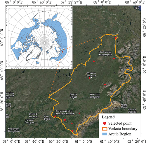
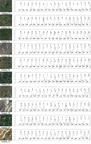
When selecting examined points, we overlay with the rasterization of Circumpolar Arctic Vegetation Map (CAVM) (Raynolds et al. 2019) product for reference. The rasterization of CAVM product was produced in 2003, and divided the Arctic circle into 16 vegetation types, glacier, saline water, freshwater, and non-Arctic land, which is available at https://www.geobotany.uaf.edu. Therefore, we select the examined points within vegetation area. The selected 10 points with its high resolution image and the NDVI time series curves during 2003–2021 are shown in Figure 2.

Figure 2. The NDVI time series during 2003–2021 of the selected ten vegetation points.

Meanwhile, we also downloaded the MODIS images in the whole Vorkuta, and used TSR-PT method to reconstruct all the pixels in Vorkuta, to realize a spatial continuous and temporal continuous Arctic vegetation NDVI map, for studying the spatial-temporal dynamic of Arctic vegetation structure.

3. Methods

3.1. Overview

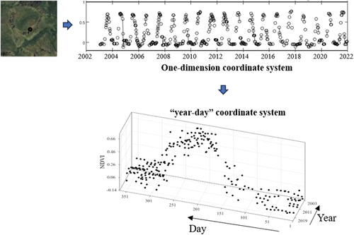
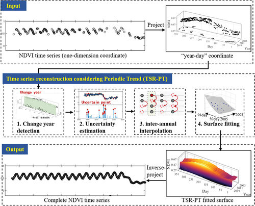
In order to fully utilize the NDVI information during the same phenological period across different years to interpolate missing observations in the current year, we project the one-dimensional time-series data onto a two-dimensional coordinate space, with “day” as the x-axis, “year” as the y-axis, and NDVI value as the z-axis, forming a “year-day” coordinate system. Subsequently, following the traditional filtering process of curve fitting method in one-dimensional space, this study conducted surface fitting on two-dimensional coordinate system for NDVI reconstruction. This can effectively account for the phenological information in other years.

Traditional one-dimension polynomial fitting usually takes the temporally adjacent observations within a certain time range as input, and utilizes least square method to derive the polynomial weights. The derived polynomial function can then be used to predict the missing observation and achieve a complete time series NDVI. The formula is as follows:

(1) $\mathit{y}=a_0+a_1\mathit{x}+a_2{x}^2+\dots +a_N{x}^N$(1)

where $\mathit{x}$ represents the day of year from 1 to 365, $\mathit{y}$ is the observed NDVI value, $a_0\dots a_n$ are the polynomial weights, and $\mathit{N}$ is the power order of the polynomial.

Suppose $\mathit{M}$ NDVI observation is available, i.e. $\left\{x_m,y_m,\mathit{m}=1\dots \mathit{M}\right\}$ (where $x_m$ represents the DOY date, $y_m$ represents the NDVI value, $\mathit{M}>\mathit{N}$), then we can substitute these observations into the polynomial function:

(2) $\left\{\begin{array}{c}{y}_1=a_0+a_1{x}_1+a_2{x}_1^2+\dots +a_N{x}_1^N\\ y_2=a_0+a_1{x}_2+a_2{x}_2^2+\dots +a_N{x}_2^N\\ \dots \\ y_M=a_0+a_1{x}_M+a_2{x}_M^2+\dots +a_N{x}_M^N\end{array}\right.$(2)

This function group can be organized into matrix form:

(3) $\left[\begin{array}{c}{y}_1\\ \begin{array}{c}{y}_2\\ \text{.}\text{.}\text{.}\\ y_N\end{array}\end{array}\right]=\left[\begin{array}{c}\begin{array}{ccc}1& x_1& \begin{array}{ccc}{x}_1^2& \dots & x_1^N\end{array}\end{array}\\ \begin{array}{ccc}1& x_2& \begin{array}{ccc}{x}_2^2& \dots & x_2^N\end{array}\end{array}\\ \begin{array}{ccc}\text{.}\text{.}\text{.}& \text{.}\text{.}\text{.}& \begin{array}{ccc}\text{.}\text{.}\text{.}& \text{.}\text{.}\text{.}& \text{.}\text{.}\text{.}\end{array}\end{array}\\ \begin{array}{ccc}1& x_M& \begin{array}{ccc}{x}_M^2& \dots & x_M^N\end{array}\end{array}\end{array}\right]\cdot \left[\begin{array}{c}{a}_0\\ \begin{array}{c}{a}_1\\ \text{.}\text{.}\text{.}\\ a_N\end{array}\end{array}\right]\text{break}\mathit{Y}=\mathit{X}\cdot \mathit{A}$(3)

where the polynomial weights $\mathit{A}$ can be derived by least square solution:

(4) $\mathit{A}=\left(X^T\mathit{X}\right)X^T\mathit{Y}$(4)

Finally, given a missing observation at date $x_t$, the NDVI of this date ${y_t}^{\prime }$can be predicted by:

(5) ${y_t}^{\prime }=a_0+a_1{x}_t+a_2{x}_t^2+\dots +a_N{x}_t^N$(5)

In this study, two-dimension polynomial fitting model (also known as surface fitting) is adopted based on the “year-day” coordinate (Figure 3) which not only takes temporally adjacent observations, but also includes observations from the same period in different years when large missing occurs. The function can be given as:

(6) $\mathit{z}=a_0+a_1\mathit{x}+\dots +a_n{x}^n+b_1\mathit{y}+\dots +b_m{y}^m$(6)

where $\mathit{x}$ represents the days ranged from 1 to 365, $\mathit{y}$ represents years, and $\mathit{z}$ represents NDVI value. $a_0\dots a_n$，$b_1\dots b_m$ are polynomial weight, and $\mathit{n}$ and$\mathit{m}$ are the power orders of the polynomial.

However, three main problems in surface fitting of Arctic vegetation NDVI are obvious:

1. The prerequisite of surface fitting is that if the ground objects do not change within a period of time, the observations during this period can be used to fit the surface polynomial function. For example, if vegetation converted to bare soil in year $\mathit{N}$, observations in year $\mathit{N}-1$ should not be included when fitting for years after $\mathit{N}+1$. Therefore, how to quickly detect the changed year in long-term time series is a key issue.

2. Surface fitting requires sufficient observations to achieve stable reconstruction of NDVI. Typically, the higher the order of the fitting polynomial, the closer the fitted surface will be to the true surface. A high-order polynomial means there are more coefficients to be determined, and thus, more observations are needed to ensure the polynomial is well-posed. However, remote sensing observations in the Arctic region are severely limited, resulting in a long period of continuous missing data. Fewer observations make it challenging to fit a smooth and stable surface. Therefore, appropriately interpolating missing observations prior to surface fitting to provide sufficient data for stable surface fitting is another crucial issue that needs to be addressed.

3. When using observations from adjacent temporal in the same year, or observations from the same period in different years for surface fitting, it would lead to errors in the fitted surface if there are uncertainties in the adjacent observations, and these uncertainties are difficult to detect. For example, the disturbance of vegetation by mist may lead to a slight decrease in NDVI, and this decrease is difficult to perceive, and leads to low NDVI values in the final reconstruction. Therefore, how to assess the uncertainty of each NDVI observation, and remove uncertain observations are key issues for improving the fitting accuracy.

Therefore, we start from these three issues respectively and introduce how the TSR-PT proposed in this article considers these three key factors in the reconstruction process.

Figure 3. “Year-day” coordinate system construction.

3.2. Change year detection

It is necessary to determine whether there is any land cover change during the examined time period, and only the observations within the unchanged time interval can be used for surface fitting. Although there are many approaches for long-term time-series change detection, such as continuous change detection and classification (CCDC) (Zhu and Woodcock 2014), breaks for additive season and trend (BFast) (Kennedy, Yang, and Cohen 2010; Verbesselt et al. 2010), these methods are time consuming and tend to provide false alert when the curve is contaminated with uncertainty.

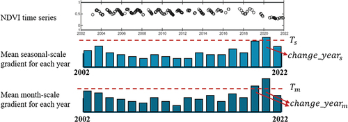
Therefore, this study proposes a fast change detection method. Assuming that the Arctic vegetation remains consistent without transitioning to other land covers in the current year and the previous year, we can expect similar periodic information in both years. To model this similarity, we employ the inter-annual gradient. Specifically, we analyze both seasonal-scale and month-scale statistics between these two years. The seasonal-scale statistic allows us to fully consider phenological variations, while the month-scale statistic enables us to capture smaller fluctuations effectively. The calculation pipeline is shown in Figure 4, and formula is as follows:

Figure 4. Seasonal-scale and month-scale NDVI gradient calculation between different years.

(7) $\mathit{Gradian}{t}_{s_n}^{\mathit{N}+1}=\frac{NDV{I}_{s_n}^{\mathit{N}+1}-\mathit{NDV}{I}_{s_n}^{\mathit{N}}}{\mathit{NDV}{I}_{s_n}^{\mathit{N}}},\mathit{n}=1\dots 4$(7)

(8) $\mathit{Gradian}{t}_{m_n}^{\mathit{N}+1}=\frac{NDV{I}_{m_n}^{\mathit{N}+1}-\mathit{NDV}{I}_{m_n}^{\mathit{N}}}{\mathit{NDV}{I}_{m_n}^{\mathit{N}}},\mathit{n}=1\dots 12$(8)

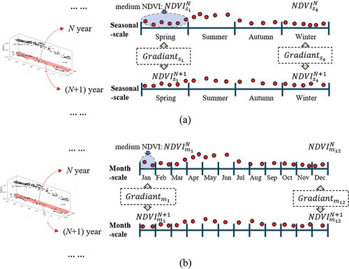
where $\mathit{Gradian}{t}_{s_n}^{\mathit{N}+1}$ represents the gradient between the NDVI in $S_n$ season at $\left(\mathit{N}+1\right)$ year and the NDVI in $S_n$ season at $\mathit{N}$ year，$\mathit{Gradian}{t}_{m_n}^{\mathit{N}+1}$ represent the gradient between the NDVI in $m_n$ month at $\left(\mathit{N}+1\right)$ year，and NDVI in $S_m$ month at $\mathit{N}$ year. $\mathit{NDV}{I}_{s_n}^{\mathit{N}+1}$ and $\mathit{NDV}{I}_{s_n}^{\mathit{N}}$ respectively represent median value of NDVI within $S_n$ season at $\left(\mathit{N}+1\right)$ year and $\mathit{N}$ year, $\mathit{NDV}{I}_{m_n}^{\mathit{N}+1}$ and $\mathit{NDV}{I}_{m_n}^{\mathit{N}}$ respectively represent median value of NDVI within $m_n$ month at $\left(\mathit{N}+1\right)$ year and $\mathit{N}$ year.

Finally, we use the average value of the four seasonal-scale gradients $\mathit{Gradian}{t}_{s_n}^{\mathit{N}}$ and twelve month-scale gradients $\mathit{Gradian}{t}_{m_n}^{\mathit{N}}$ as the final indicators for determining the probability of sudden change.

(9) $\mathit{mean}\_\mathit{Gradian}{t}_s^{N+1}=\frac{1}{4}\times \sum _{\mathit{n}=1}^4\mathit{Gradian}{t}_{s_n}^{\mathit{N}+1}$(9)

(10) $\mathit{mean}\_\mathit{Gradian}{t}_m^{N+1}=\frac{1}{12}\times \sum _{\mathit{n}=1}^{12}\mathit{Gradian}{t}_{m_n}^{\mathit{N}+1}$(10)

Generally, the larger the gradient, the greater the probability of changes occurring between $\left(\mathit{N}+1\right)$ year and $\mathit{N}$ year. However, how can we determine the appropriate threshold for the gradient to accurately assess whether a land cover change has occurred? To address this, we employ the OSTU algorithm to determine an adaptive threshold. The OSTU algorithm, which stands for Optimal Inter-Class Variation, is a method that aims to maximize the difference between different classes.

Supposing that there exist an optimal threshold T, which can divide all the seasonal-scale gradients into two categories, “unchanged” (less than T) and “changed” (greater than T). In this way, the mean gradient of these two categories can be calculated as $m_u$, $m_c$. Assuming that the mean gradient of all the seasonal-scale gradients within the examined NDVI time series is $m_g$, and a certain gradient being classified as “changed” and “unchanged” are $p_c$ and $p_u$, the equation can be established:

(11) $p_c\cdot m_c+p_u{m}_u=m_g$(11)

(12) $p_c+p_u=1$(12)

According to the variance calculation, the inter-class variance between the gradients representing “change” and “unchanged” is:

(13) ${\sigma }^2=p_c{\left(m_c-m_g\right)}^2+p_u{\left(m_u-m_g\right)}^2$(13)

We simplify the above equation and substitute Equation (11)(11) $p_c\cdot m_c+p_u{m}_u=m_g$(11) into Equation (13)(13) ${\sigma }^2=p_c{\left(m_c-m_g\right)}^2+p_u{\left(m_u-m_g\right)}^2$(13) :

(14) ${\sigma }^2=p_c{p}_u{\left(m_c-m_u\right)}^2$(14)

After that, we search for the threshold $\mathit{T}$ within the range of −1 to 1, incrementing it by 0.1 steps until we find a $\mathit{T}\mathit{\hspace{0.17em}}$that maximizes ${\sigma }^2$. This T is the optimal threshold for determining whether a gradient represents sudden change or not. The same strategy can be applied to determine the threshold of the month-scale gradient.

Assuming that the derived thresholds for the seasonal-scale gradient and the month-scale gradient are $\mathit{T}{ }_s$ and $\mathit{T}{ }_m$, we can identify the years of sudden changes during the examined time series (e.g. 2003–2022). To ensure the robustness of change year identification, we take the intersection of from two for the final determination (Figure 5).

Figure 5. Change year determination by OSTU threshold and intersection of two change_year sets.

In fact, based on a large number of experiments on Arctic vegetation, we have summarized an additional set of threshold conditions to screen changed years to further ensure robustness (as shown in Table 1). The main variables considered include the variance of NDVI seasonal-scale gradient $\mathit{va}{r}_s$, the variance of NDVI month-scale gradient $\mathit{va}{r}_m$, sum of seasonal-scale and month-scale gradients $\mathit{su}{m}_{\mathit{s}+\mathit{m}}$, mean of the seasonal-scale gradient $\mathit{mean}\_\mathit{gra}{d}_s$, mean of the month-scale gradient $\mathit{mean}\_\mathit{gra}{d}_m$. The specific thresholds for each variable are as follows:

Because gradient calculation and threshold screening are much faster than traditional curve fitting or morphological curve segmentation, it can achieve rapid change year detection in long-term time series.

3.3. Inter-annual interpolation

To appropriately interpolate missing observations before surface fitting to ensure sufficient observations for well-posed fitting, this study first identifies the unchanged interval within the examined NDVI time series, based on the change year obtained in the previous step. Within this unchanged interval, observations from the same period in different years are used to interpolate missing observations in the current year. The specific steps and formulas are outlined in Figure 6.

Figure 6. The process of inter-annual interpolation.

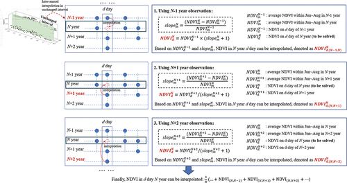
Suppose we need to interpolate the missing NDVI on $\mathit{d}$ day in $\mathit{N}$ year. First, we observe whether there are observations on $\mathit{d}$ day in other years within the unchanged interval, and includes them into the stack for subsequent calculations. For example, as shown in Figure 6, there are NDVI observations for years $\mathit{N}-1$, $\mathit{N}+1$, and $\mathit{N}+2$ on $\mathit{d}$ day, i.e. $\mathit{NDV}{I}_d^{N-1}$，$\mathit{NDV}{I}_d^{N+1}$，$\mathit{NDV}{I}_d^{N+2}$, and these observations can be used to interpolate a reasonable NDVI observation on $\mathit{d}$ day in $\mathit{N}$ year.

Taking the interpolation from year $\mathit{N}-1$ to year $\mathit{N}$ as an example, first, the slope $\mathit{slop}{e}_m^N$ from year $\mathit{N}$ to year $\mathit{N}-1$ is derived, and then, based on this slope, the $\mathit{NDV}{I}_d^{N-1}$ can be converted to $\mathit{NDV}{I}_d^N$, as shown in the first row in Figure 6. Among the equation, $\mathit{NDV}{I}_m^N$ represents the average NDVI of the season corresponding to day $\mathit{d}$ at year $\mathit{N}$. Multiple NDVI values can be obtained through multiple inter-annual observation, and the final NDVI value on day $\mathit{d}$ at year $\mathit{N}$ can be derived by averaging.

3.4. Uncertainty estimation

The uncertainty existing in the NDVI observation would deviate the surface fitting as well as the inter-annual interpolation. Therefore, it is necessary to assess the uncertainty of each NDVI observation and remove the uncertain one beforehand.

Generally, if an NDVI observation is affected by mist or imaging noise, its distance from the line connecting the observations at previous and subsequent temporal will be relatively far. Besides, there may also be differences between it and the observation at the same period in different years. Therefore, this study proposes two uncertainty assumptions and constructs an uncertainty evaluation metrics based on these assumptions, i.e. 1) the greater the residual between the observed value and the fitted value in the current year, the larger the uncertainty; 2) the greater the gradient between the observations at same period in different years, the larger the uncertainty. The uncertainty modeling is shown in Figure 7.

Figure 7. Two assumptions for evaluating the uncertainty of each observation.

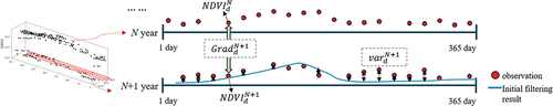
Supposing that we need to assess the uncertainty on d day at $\left(\mathit{N}+1\right)$ year, according to the assumption 1, we first calculate the inter-annual gradient on this date, and the greater the gradient, the larger the uncertainty, which can be given as:

(15) $\mathit{Gra}{d}_d^{N+1}=\left(\mathit{NDV}{I}_d^{N+1}-\mathit{NDV}{I}_d^N\right)/\mathit{NDV}{I}_d^N$(15)

After then, based on the assumption 2, we calculate the residual between observed value and the fitted value on this date, and the greater the residual, the larger the uncertainty, which can be given as:

(16) $\mathit{va}{r}_d^{N+1}={\left(NDV{I}_d^{N+1}-\mathit{S}{G}_d^{N+1}\right)}^2$(16)

Considering the monotonicity of both metrics $\mathit{Gra}{d}_d^{N+1}$ and $\mathit{va}{r}_d^{N+1}$, and their proportionality to uncertainty, the two metrics can be combined by multiplying them, and we can obtain the uncertainty of each observation. Finally, all the observations can be classified into two categories, i.e. certainty and uncertainty, based on the uncertainty probability threshold (adaptively calculated based on the OSTU method), and the uncertainty observations would be eliminated during surface fitting and inter-annual interpolation, thereby improving the smoothness of the fitting process.

The whole pipeline of the proposed TSR-PT method for NDVI reconstruction is provided in Figure 8, which is consist of sequential key techniques of change year detection, uncertainty estimation, inter-annual interpolation and surface fitting.

Figure 8. The pipeline of the proposed TSR-PT method for NDVI reconstruction.

3.5. Experiment setting

3.5.1. Synthetic data experiment

To validate the effectiveness of the proposed TSR-PT for reconstructing NDVI time series of Arctic vegetation, we designed a synthetic data experiment. Firstly, we selected ten data points with relatively less missing values in the Vorkuta study area from MODIS observations, and then used a simple interpolation method to complete them, which was then used as the reference for accuracy assessment. Secondly, we randomly masked 70%, 60%, 50%, and 40% of the observations on the reference during the 2003 to 2021, to simulate missing data. Finally, we used TSR-PT to reconstruct all NDVI observations every 8-days from 2003 to 2021, and evaluate the accuracy using the reference before masking.

Besides, we selected SG filtering, FFT filtering, and BISE filtering methods for comparison. The SG filtering algorithm divides the NDVI time series into several windows, and performs polynomial fitting within each window. The advantage is that it can effectively remove noise and interference, preserving the main features and trends of the NDVI time series. The disadvantage is that the polynomial fitting requires the selection of an appropriate window size and polynomial order, and inappropriate parameters may lead to fitting failure.

The FFT filtering algorithm transforms the NDVI time series from the time domain to the frequency domain. In the frequency domain, the NDVI time series can be represented as a superposition of different frequency components, and then noise and interference can be filtered out through low-pass filtering. Finally, the filtered data are processed by the inverse Fourier transform to generate a new noise-free NDVI time series. FFT is simple and its reconstruction curve is very smooth, performs poorly for non-stationary time series due to the strict symmetry of the formula, and thus is not suitable for abrupt changes.

The BISE algorithm calculates the slope of time series data to reflect the trend of changes. It uses a first-order difference method to calculate the slope between two adjacent data points, and selects the optimal slope as the filtering result. Its advantage lies in its simplicity and does not require preset parameters, and can effectively remove short-term noise while preserving long-term trends. However, the BISE algorithm also has some shortcomings. If there are outliers or drastic fluctuations in the time series data, it may affect its effectiveness.

In terms of quantitative accuracy evaluation, the NDVI reconstructed from each time phase can be compared with its corresponding true pixel NDVI to calculate the root mean square error (RMSE). The average of the RMSE for all observed time phases is used as the quantitative accuracy of each algorithm.

3.5.2. Application experiment

In practical applications, the time-series NDVI curve in unit of points is difficult to reflect the spatial distribution and dynamic changes of Arctic vegetation structure. To observe the spatial evolution of Arctic vegetation structure, especially their spatial distribution and boundaries, we used the TSR-PT method to reconstruct the NDVI time series of all MODIS pixels in the Vorkuta region, and based on the spatial distribution of Arctic vegetation in NDVI time series map, to analyze the spatiotemporal dynamics of Arctic vegetation structure.

4. Experiment results and analysis

4.1. Validation experiment in terms of NDVI curve

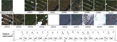
Figure 9 shows the 30 m resolution Landsat remote sensing images merged within April to September each year at vorkuta_01 location from 2003 to 2021 (including the Sentinel-2 images merged within April to September after 2016), which are used for visual inspection of whether there have changes occurred at vorkuta_01 location, and can verify the effectiveness of the proposed change year detection. Noteworthy is that due to the lack of data from Landsat-4, Landsat-5, and Landsat-8 in the Arctic region during this time series, we incorporated the Landsat-7 for merging, which have been contaminated by striping effects, and thus resulting in striping in part of the years in Figure 9. At the same time, it can also be found that there was a serious lack of observation in 2015, while 2018 and 2019 were covered by snow for a longer period of time. The missing rate of the original NDVI time series observation at vorkuta_01 location is 29.52%. The missing rate is calculated based on the standard 46 observations per year from 2003 to 2021.

Figure 9. High resolution visual examination of the Vorkuta_01 during 2003–2021.

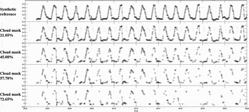
To make the subsequent accuracy evaluation convenient, we completed the missing temporal observation by simple interpolation, to synthesize a “reference” for the subsequent accuracy assessment. Then, according to the experimental setting in Section 3.5, we randomly mask observations on the synthesized reference to simulate missing observation situation. Figure 10 shows the NDVI time series under four observation missing situations with mask ratios of 21.05%, 45.08%, 57.78%, and 72.65%. As can be seen, when the missing rate reaches over 70%, it is difficult to discern the periodic fluctuation pattern of vegetation.

Figure 10. The synthetic reference and synthetic time series with different degree of cloud mask.

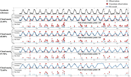
Firstly, change year detection process is performed. It should be noted that the change detection is conducted on all the four situations with different cloud masked ratios. We found that there is no land cover change during 2003 to 2021 at Vorkuta_01 location, which is also confirmed by visual interpretation of the time-series image in Figure 11. Secondly, the uncertainty observations were eliminated by observation uncertainty estimation procedure. Figure 11 shows the uncertainty estimation of all the observations obtained under four different cloud mask situations, as well as the eliminated uncertainty observations (denoted as red point). It can be found that the uncertain observations usually occurred in the temporal with large residuals from the SG fitting curve.

Figure 11. Observation uncertainty estimation for different cloud mask situation.

After removing the uncertain observations, we performed inter-annual interpolation and surface fitting to obtain the final TSR-PT results, which were then compared with the results of other algorithms, as shown in Figure 12. From perspective of inspection, the NDVI time series reconstructed by TSR-PT is the most similar to the reference time series. Besides, even during the most severely missing period from 2016 to 2018, TSR-PT can still reconstruct the phenological fluctuations of Arctic vegetation well, as shown in the red circle in Figure 12. This effect is due to the fact that our method extends the traditional one-dimensional filtering algorithm that only considers intra-year neighborhoods to a surface filtering algorithm that considers both intra-year neighborhoods and inter-year neighborhoods. By borrowing phenological information from other years, TSR-PT is able to compensate for the current year’s observations and recover relatively complete vegetation phenological characteristics under extreme missing conditions.

Figure 12. Comparison of the NDVI time series reconstruction result of each algorithm on 72.65% cloud mask situation, as well as the RMSE of each predicted observation.

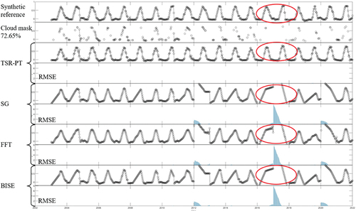
But other algorithms are not as satisfactory, especially during the serious missing period of 2016 to 2018. Due to the extreme lack of observations, it is difficult to obtain suitable polynomial parameters for methods such as the least squares fitting-based SG filter; For frequency domain transformation method like FFT filtering, accurate decomposition of frequency signals is difficult with fewer observations. For first-order derivative-based method like BISE filtering algorithms, lack of observations would make it difficult to obtain the optimal gradient.

At the same time, we zoomed-in single years of 2008 and 2020 for visual inspection of detailed curve reconstruction, as shown in Figure 13. It can be seen that most observations in spring, summer, and autumn in middle 2008 were missing, leaving only a few observations at the beginning and end of the year, resulting in a curve trend that does not properly reflect the phenological fluctuations of Arctic vegetation. Therefore, traditional methods such as SG, FFT, and BISE filtering methods that are based on only a few observations failed to reconstruct the real phenological fluctuation of the time series curve, such as the greening and withering of Arctic vegetation during spring, summer, and autumn.

Figure 13. Comparison of the NDVI time series reconstruction result in single year on 72.65% cloud mask situation, to examine the detail performance.

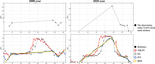
As for the year of 2020, there were no observations in the first half year, and one observation at the end of summer, most of the observations are concentrated in autumn and winter. This curve trend is also disturbed and cannot reflect the true fluctuation of vegetation phenology. Traditional filtering methods tend to fit the shape of the curve based on the existing observations, and thus making it difficult to recover the true phenological trend.

By contrast, the proposed TSR-PT can reconstruct the severely missing values in current year with the help of other years within the invariant interval (as the red line in Figure 13), which is the closest to the black line reference. It can reconstruct the trend of NDVI during the growth and decline of vegetation in one year, which is very important for monitoring Arctic vegetation. For example, by reconstructing continuous NDVI time series, the start of growing season (SOS) and end of growing season (EOS) of Arctic vegetation can be obtained, and whether the phenological growth period of Arctic vegetation has increased or decreased can be determined, thus reflecting seasonal climate changes in the Arctic. The reconstruction analysis for other Vorkuta_02 ~ 10 point data is similar and is not repeated here.

Table 2 shows the quantitative evaluation of the reconstruction results at Vorkuta_01 location, by comparing with the SG, FFT, and BISE algorithms, under four different cloud mask situations. It can be found that in scenarios where cloud cover is relatively small, the RMSE of our proposed algorithm is relatively worse than traditional methods such as SG. The reason is that the traditional methods tend to fit the shape of the curve by existing observations. For example, in the absence of ~21% and ~45% observations, the curve is relatively complete, and therefore traditional methods have better fitting results. However, the TSR-PT algorithm tends to rely on observations from the same period in different years, which may inevitably cause interference from observations of the other years on the fit of the current year.

Table 1. Additional controllable variables that further help for change year determination.

Controllable variable	Threshold
$\mathrm{va}{\mathrm{r}}_{\mathrm{s}}$	<0.1
$\mathrm{va}{\mathrm{r}}_{\mathrm{m}}$	<0.1
$\mathrm{su}{\mathrm{m}}_{\mathrm{s}+\mathrm{m}}$	>3.0
$\mathrm{mean}\mathrm{\_}\mathrm{gra}{\mathrm{d}}_{\mathrm{s}}$	>0.15
$\mathrm{mean}\mathrm{\_}\mathrm{gra}{\mathrm{d}}_{\mathrm{m}}$	>0.15
Determination	Changed

When the missing observations are severe, such as ~72%, the outline of the curve depicted by the existing observations can no longer represent the true phenological cycle of vegetation. On this circumstance, traditional methods such as SG filtering would perform erroneous fitting based on the unrepresentative observed value, and the RMSE accuracy of SG is 0.2482, the FFT accuracy is 0.2369, and the BISE accuracy is 0.2483. By contrast, the TSR-PT algorithm can reconstruct a more realistic Arctic vegetation phenological cycle under severe missing observation, with an RMSE accuracy of 0.0089, which is more than 10 times better than traditional methods, since TSR-PT used observations from the same period in different years in the absence of extreme data in the current year.

Table 2. Quantitative assessment of each algorithm on Vorkuta_01 under four different cloud mask situations.

RMSE	Cloud mask rate
	~21%	~45%	~58%	~72%
SG	0.0009	0.0018	0.0086	0.2482
FFT	0.0015	0.0020	0.0078	0.2369
BISE	0.0010	0.0018	0.0086	0.2483
TSR-PT	0.0072	0.0087	0.0087	0.0089

Table 3 shows the quantitative evaluation accuracy of the reconstruction results at Vorkuta_02 ~ 10 locations under ~72% extreme missing conditions, and it can be found that our method achieves the best accuracy in RMSE on all the 10 locations.

Table 3. Quantitative assessment of each algorithm on Vorkuta_02 ~ 10 under ~70% cloud mask situation.

RMSE	Could mask rate of ~70%
	V02	V03	V04	V05	V06	V07	V08	V09	V10
SG	0.1270	0.0275	0.0079	0.0145	0.0027	0.0183	0.1669	0.0035	0.0058
FFT	0.1209	0.0256	0.0082	0.0133	0.0025	0.0171	0.1674	0.0031	0.0051
BISE	0.1270	0.0320	0.0078	0.0224	0.0101	0.0262	0.1708	0.0056	0.0195
TSR-PT	0.0049	0.0037	0.0066	0.0032	0.0013	0.0118	0.0106	0.0009	0.0008

4.2. Spatial-temporal analysis of Arctic vegetation structure

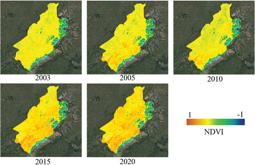
We used the TSR-PT method to reconstruct the NDVI time series of all MODIS pixels in the Vorkuta region, and Figure 14 shows the reconstructed NDVI maps in 2003, 2005, 2010, 2015, 2020, which used the observations in July.

Figure 14. The reconstructed NDVI maps in five years within July.

In order to distinguish the tree from the tundra to inspect the spatial distribution of vegetation structure, we select a threshold of NDVI and reclassified Figure 14 into tree map (including tree and shrub-tundra) or non-tree map (including moss, lichen, and grass), as shown in Figure 15. Based on the previous study that distinguishing different types of vegetation, we select the 0.7 as the threshold, where the pixels with NDVI larger than 0.7 will be regarded as tree and shrub-tundra, and that smaller than 0.7 will be regarded as moss, lichen, and grass.

Figure 15. The reclassified maps by harden the NDVI maps with threshold.

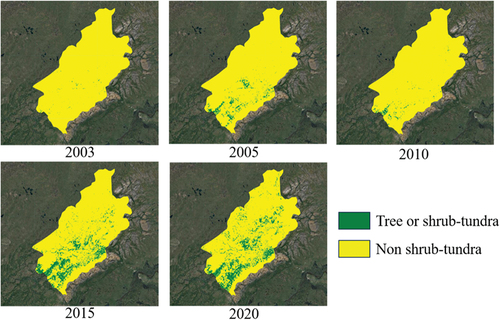
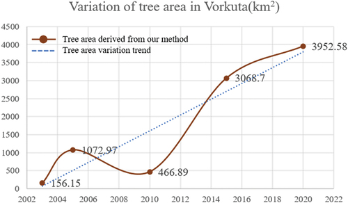
We make a statistic of the tree area in Vorkuta during these five years, and the result is shown in Figure 16. We find that since 2003, the Arctic tree area has continued to increase, which encroached the tundra. Until around 2020, the vegetation area in Vorkuta experience up to over 20 folds increase. In order to quantitatively validate the derived area, we made an area statistic of the WorldCover product, which is produced by European Space Agency (ESA). The area of tree or shrub-tundra from our reconstruction result in 2020 is 3952.58 km², which is close to the area of tree cover and shrubland derived from WorldCover, i.e. 3819.19 km².

Figure 16. Variation of tree area in Vorkuta.

The Arctic vegetation structure in terms of growing range refers to the highest latitude or altitude where plants can continue to grow. In the Arctic Circle, this range roughly corresponds to the highest latitude where vegetation can thrive. As the climate warms, shrubs and forests are moving northward, leading to an ever-expanding forest area in the Arctic Circle and a longer growth cycle (Lloyd and Fastie 2003). The continuous expansion of the forest would promote carbon storage in the soil and increase temperatures (Zhuang et al. 2023), ultimately melting the permafrost (Zhang et al. 2013). Most of the Earth’s methane greenhouse gases are trapped in the permafrost. Once this greenhouse gas, which is over ten times more powerful than carbon dioxide, is released, it would exacerbate global warming, thus creating a vicious cycle.

According to existing research, vegetation structure in the Arctic has moved northward by tens of kilometers over the past half century. As the forest area expands, it may have an impact on local wildlife habitats and migration routes, thereby affecting biodiversity and the stability of ecosystems.

5. Discussion

5.1. The effectiveness of the TSR-PT

The experimental results of the continuous missing observations reconstruction in the Arctic vegetation scene have demonstrated the superiority of the proposed method. The reason can be own to the fact that our method extends the traditional one-dimensional function fitting to two-dimensional surface fitting, which takes into account both intra-year and inter-year neighborhoods. By incorporating phenological information from previous years, TSR-PT is able to compensate for the current year’s observations and recover relatively complete vegetation phenological characteristics even under extreme missing conditions (Yan and Roy 2018). In contrast, other one-dimensional function fitting methods failed to accomplish the challenging reconstruction task. Specifically, when confronted with continuous missing scene with insufficient observations, SG filter is difficult to obtain suitable polynomial parameters, FFT is difficult to predict an accurate decomposition of frequency signals, and BISE is difficult to obtain the optimal gradient.

From the experimental results in time series NDVI map reconstruction in Vorkuta region, we find that since 2003, the Arctic forest area has continued to expand from lower latitude to higher latitude, i.e. expand from the south of Vorkuta to the north, which encroached the tundra. The reason behind it is that Vorkuta is a transition region of Arctic tundra and forest, which is one the best place for monitoring vegetation structure variation (Andreyev 1936), and as the climate warmed over the past half century, shrubs and forests are moving northward (Lloyd and Fastie 2003). This finding demonstrated the advantage of the proposed TSR-PT in continuous spatial-temporal dynamic monitoring of the vegetation structure. Besides, NDVI values can also reflect the dates of snow accumulation and melting in each year, which can indirectly indicate the climate change.

5.2. Limitations and future aspect

Although the superiority of the TSR-PT under severe missing situation is obvious, the limitations are also nonnegligible, which can be summarized in two folds:

1. First, in scenarios where cloud cover is relatively minimal (e.g. circa 20% or 45%), the TSR-PT performs relatively poorly compared with the traditional methods such as SG filtering in quantitative assessment. The reason is that less cloud coverage implies more continuous observations with clear curve contour, and SG filtering that relies temporally adjacent observations for fitting can better approximate the shape trend of the curve. In contrast, the TSR-PT relies heavily on observations from the same period in different years, which may unavoidably introduce interference from observations of other years on the fit of the current year. In the future, we will further dedicate to alleviate this drawback by developing robust uncertainty estimation strategy to eliminate interference.

2. Second, most of the current TSR algorithms conduct quantitative accuracy evaluation based on the degree of similarity with the ground reference curve, ignoring the quantification in terms of essential characteristics of NDVI. Indeed, time series NDVI usually showed regular periodic fluctuations within a year, and this fluctuation is consistent with the phenological cycles of vegetation, such as sprout, growth, and withering. Therefore, in the future, we will further dedicate to establish a phenological metric for further quantitative examination of each algorithm.

In the future development of TSR algorithms for NDVI in the Arctic region, the TSR-PT model has great potential to realize seamless NDVI times series products, which is indicative for monitoring spatial variation of Arctic vegetation structure, and can facilitate greater understanding of the correlation between vegetation structure change and climate change in the Arctic Circle.

6. Conclusions

This study developed a Time Series Reconstruction method considering Periodic Trend (TSR-PT) to alleviate the severe missing NDVI observation condition in Arctic region, and realize continuous spatial-temporal dynamics monitoring of Arctic vegetation structure. TSR-PT reconstructs missing observations by “borrowing” phenological feature from the other unchanged years, which is achieved by two dimensional “year-day” coordinate data and inter-annual correlation modeling based on surface fitting function. Specifically, TSR-PT uses inter-annual gradients for separate phenological change and trend change within the incomplete NDVI time series, and the trend change is used for discovering unchanged interval, the phenological change is used for inter-annual interpolation, and surface fitting is adopted for final reconstruction.

In experiment part, we explore its usability in Vorkuta region which is the transition zone of vegetation in the Arctic Circle based on MODIS data, and find that the proposed TSR-PT is able to reconstruct NDVI with reasonable phenological feature even the missing rate reaches over 70%, which was usually falsely constructed by traditional filtering or fitting method, and suppress them by 0.038 in terms of RMSE; besides, we find that since 2001, the Arctic shrub and forest have continued to increase and encroach the original tundra ecosystem, with an area growth rate of averagely 15% per year northward, which caused a largely Arctic vegetation structural change.

We hope that the proposed TSR-PT can facilitate the spatial-temporal dynamics monitoring of Arctic vegetation structure and promote further research on the causation of global warming and Arctic biome ecosystems

Disclosure statement

No potential conflict of interest was reported by the author(s).

Data availability statement

The data that support the findings of this study are available from the corresponding author, [Da, He], upon reasonable request.

Additional information

Funding

This study was supported in part by the National Natural Science Foundation of China under [grant number 42222106], [grant number 61976234], and [grant number 42201340].

Notes on contributors

Zihong Liu

Zihong Liu received a B.S. degree in physical geography from Beijing Forestry University, Beijing, China, in 2022. She is currently pursuing M.S. degree from the School of Geospatial Engineering and Science, Sun Yat-sen University, Zhuhai, China. Her research interests include the response and changes of Arctic Vegetation related to Climate Change.

Da He

Da He received a B.S. degree in remote sensing science and technology and Ph.D. degree in photogrammetry and remote sensing from Wuhan University, China, in 2015 and 2020, respectively. Since 2023, he has been working as an associate professor in the School of Geography and Planning, Sun Yat-Sen University, Guangzhou, China. He has published more than 20 research papers in international journals, such as Remote Sensing of Environment, Transactions on Geoscience and Remote Sensing. His current research interests include multi- and hyper-spectral remote sensing image classification, deep learning, data fusion, and change detection.

Qian Shi

Qian Shi received a B.S. degree in science and techniques of remote sensing from Wuhan University, Wuhan, China, in 2010, and Ph.D. degree in photogrammetry and remote sensing from the State Key Laboratory of Information Engineering in Surveying, Mapping and Remote Sensing, Wuhan University, in 2015. She is currently a full professor in the School of Geography and Planning, Sun Yat-sen University, Guangzhou, China. Her research interests include remote sensing image classification, including deep learning, active learning, transfer learning.

Xiao Cheng

Xiao Cheng received B.E. and M.Tech. degrees in engineering survey from Wuhan Technical University of Surveying and Mapping, Wuhan, China, in 1998 and 2001, respectively, and the Ph.D. degree in cartography and geographical information system from the Graduate School, Chinese Academy of Sciences, Beijing, China, in 2004. In 2004, he joined the Institute of Remote Sensing Applications, Chinese Academy of Sciences, as an assistant researcher, where he became an associate researcher in 2008. In 2009, he moved to Beijing Normal University (BNU), Beijing, and served as the Associate Dean of the College of Global Change and Earth System Science (GCESS), BNU, and became a professor. In 2016, he became the Dean of GCESS. In 2019, he joined Sun Yat-sen University, Zhuhai, China, initiated the School of Geospatial Engineering and Science (SGES), and acts as the Dean. He has published over 100 peer-reviewed journal articles, including the Proceeding of the National Academy of Sciences, Remote Sensing of Environment, and other top international geoscience journals. His research interests include polar remote sensing technology and climate change in polar regions. Dr. Cheng was granted the Award for Advanced Individual of China’s Polar Exploration in 2017.

References

- Andreyev, V. 1936. “Rastitelnost’i prirodnye rayony vostochnoy chasti Bol’shezemel’skoy tundry [Vegetation and Natural Regions in the Eastern Part of the Bol’shezemel’skaya Tundra].” Trudy Polyarnoy komissii [Works of the Polar Commission] 22:1–97.
- Anisimov, O., Y. L. Zhiltcova, and V. Y. Razzhivin. 2015. “Predictive Modeling of Plant Productivity in the Russian Arctic Using Satellite Data.” Izvestiya Atmospheric and Oceanic Physics 51:1051–1059. https://doi.org/10.1134/S0001433815090042.
- Beck, P. S., C. Atzberger, K. A. Høgda, B. Johansen, and A. K. Skidmore. 2006. “Improved Monitoring of Vegetation Dynamics at Very High Latitudes: A New Method Using MODIS NDVI.” Remote Sensing of Environment 100 (3): 321–334.
- Beck, P. S., and S. J. Goetz. 2011. “Satellite Observations of High Northern Latitude Vegetation Productivity Changes Between 1982 and 2008: Ecological Variability and Regional Differences.” Environmental Research Letters 6 (4): 045501.
- Bhatt, U. S., D. A. Walker, M. K. Raynolds, P. A. Bieniek, H. E. Epstein, J. C. Comiso, J. E. Pinzon, C. J. Tucker, and I. V. Polyakov. 2013. “Recent Declines in Warming and Vegetation Greening Trends Over Pan-Arctic Tundra.” Remote Sensing 5 (9): 4229–4254.
- Chapin, F. S., III, M. Sturm, M. C. Serreze, J. P. McFadden, J. Key, A. H. Lloyd, A. McGuire, et al. 2005. “Role of Land-Surface Changes in Arctic Summer Warming.” Science 310 (5748): 657–660.
- Chen, Y., R. Cao, J. Chen, L. Liu, and B. Matsushita. 2021. “A Practical Approach to Reconstruct High-Quality Landsat NDVI Time-Series Data by Gap Filling and the Savitzky–Golay Filter.” Isprs Journal of Photogrammetry & Remote Sensing 180:174–190. https://doi.org/10.1016/j.isprsjprs.2021.08.015.
- Chen, J., P. Jönsson, M. Tamura, Z. Gu, B. Matsushita, and L. Eklundh. 2004. “A Simple Method for Reconstructing a High-Quality NDVI Time-Series Data Set Based on the Savitzky–Golay Filter.” Remote Sensing of Environment 91 (3–4): 332–344.
- Elmendorf, S. C., G. H. Henry, R. D. Hollister, R. G. Björk, N. Boulanger-Lapointe, E. J. Cooper, J. H. Cornelissen, et al. 2012. “Plot-Scale Evidence of Tundra Vegetation Change and Links to Recent Summer Warming.” Nature Climate Change 2 (6): 453–457.
- IPCC. 2014. Climate Change 2014: Contribution of Working Groups I. II and III to the Fifth Assessment Report of the Intergovernmental Panel on Climate Change. Geneva, Switzerland.
- Jia, D., C. Cheng, S. Shen, and L. Ning. 2022. “Multitask Deep Learning Framework for Spatiotemporal Fusion of NDVI.” IEEE Transactions on Geoscience & Remote Sensing 60:1–13. https://doi.org/10.1109/TGRS.2021.3140144.
- Jonsson, P., and L. Eklundh. 2002. “Seasonality Extraction by Function Fitting to Time-Series of Satellite Sensor Data.” IEEE Transactions on Geoscience & Remote Sensing 40 (8): 1824–1832.
- Kennedy, R. E., Z. Yang, and W. B. Cohen. 2010. “Detecting Trends in Forest Disturbance and Recovery Using Yearly Landsat Time Series: 1. LandTrendr — Temporal Segmentation Algorithms.” Remote Sensing of Environment 114 (12): 2897–2910. https://doi.org/10.1016/j.rse.2010.07.008.
- Lange, M., B. Dechant, C. Rebmann, M. Vohland, M. Cuntz, and D. Doktor. 2017. “Validating MODIS and Sentinel-2 NDVI Products at a Temperate Deciduous Forest Site Using Two Independent Ground-Based Sensors.” Sensors 17 (8): 1855.
- Li, T., H. Shen, Q. Yuan, and L. Zhang. 2020. “Geographically and Temporally Weighted Neural Networks for Satellite-Based Mapping of Ground-Level PM2. 5.” ISPRS Journal of Photogrammetry & Remote Sensing 167:178–188. https://doi.org/10.1016/j.isprsjprs.2020.06.019.
- Liu, M., W. Yang, X. Zhu, J. Chen, X. Chen, L. Yang, and E. H. Helmer. 2019. “An Improved Flexible Spatiotemporal Data Fusion (IFSDAF) Method for Producing High Spatiotemporal Resolution Normalized Difference Vegetation Index Time Series.” Remote Sensing of Environment 227:74–89. https://doi.org/10.1016/j.rse.2019.03.012.
- Lloyd, A. H., and C. L. Fastie. 2003. “Recent Changes in Treeline Forest Distribution and Structure in Interior Alaska.” Ecoscience 10 (2): 176–185.
- Loranty, M. M., W. Lieberman-Cribbin, L. T. Berner, S. M. Natali, S. J. Goetz, H. D. Alexander, and A. L. Kholodov. 2016. “Spatial Variation in Vegetation Productivity Trends, Fire Disturbance, and Soil Carbon Across Arctic-Boreal Permafrost Ecosystems.” Environmental Research Letters 11 (9): 095008.
- Lu, X., R. Liu, J. Liu, and S. Liang. 2007. “Removal of Noise by Wavelet Method to Generate High Quality Temporal Data of Terrestrial MODIS Products.” Photogrammetric Engineering & Remote Sensing 73 (10): 1129–1139.
- Menenti, M., S. Azzali, W. Verhoef, and R. Van Swol. 1993. “Mapping Agroecological Zones and Time Lag in Vegetation Growth by Means of Fourier Analysis of Time Series of NDVI Images.” Advances in Space Research 13 (5): 233–237.
- Meneses-Tovar, C. L. 2011. “NDVI As Indicator of Degradation.” Unasylva 62 (238): 39–46.
- Miles, V. V., and I. Esau. 2016. “Spatial Heterogeneity of Greening and Browning Between and within Bioclimatic Zones in Northern West Siberia.” Environmental Research Letters 11 (11): 115002.
- Mumtaz, F., J. Li, Q. Liu, A. Arshad, Y. Dong, C. Liu, and J. Zhao. 2023. “Spatio-Temporal Dynamics of Land Use Transitions Associated with Human Activities Over Eurasian Steppe: Evidence from Improved Residual Analysis.” Science of the Total Environment 905 (166940). https://doi.org/10.1016/j.scitotenv.2023.166940.
- Ostu, N. 1979. “A Threshold Selection Method from Gray-Level Histograms.” IEEE Trans SMC 9:62. https://doi.org/10.1109/TSMC.1979.4310076.
- Post, E., M. C. Forchhammer, M. S. Bret-Harte, T. V. Callaghan, T. R. Christensen, B. Elberling, A. D. Fox, et al. 2009. “Ecological Dynamics Across the Arctic Associated with Recent Climate Change.” Science 325 (5946): 1355–1358.
- Prevéy, J., M. Vellend, N. Rüger, R. D. Hollister, A. D. Bjorkman, I. H. Myers‐Smith, S. C. Elmendorf, et al. 2017. “Greater Temperature Sensitivity of Plant Phenology at Colder Sites: Implications for Convergence Across Northern Latitudes.” Global Change Biology 23 (7): 2660–2671.
- Raynolds, M. K., D. A. Walker, A. Balser, C. Bay, M. Campbell, M. M. Cherosov, and F. J. Daniëls. 2019. “A Raster Version of the Circumpolar Arctic Vegetation Map (CAVM.” Remote Sensing of Environment 232:111297. https://doi.org/10.1016/j.rse.2019.111297.
- Reichle, L., H. Epstein, U. Bhatt, M. Raynolds, and D. Walker. 2018. “Spatial Heterogeneity of the Temporal Dynamics of Arctic Tundra Vegetation.” Geophysical Research Letters 45 (17): 9206–9215.
- Roerink, G., M. Menenti, and W. Verhoef. 2000. “Reconstructing Cloudfree NDVI Composites Using Fourier Analysis of Time Series.” International Journal of Remote Sensing 21 (9): 1911–1917.
- Tang, L., Z. Zhao, P. Tang, and H. Yang. 2020. “SURE-Based Optimum-Length SG Filter to Reconstruct NDVI Time Series Iteratively with Outliers Removal.” International Journal of Wavelets Multiresolution and Information Processing 18 (2): 2050001.
- Taskaev, G. 1977. “Atlas Respubliki Komi po klima-tu i gidrologii [Atlas of the Komi Republic on climate and hydrology].” Moscow: Drofa.
- Verbesselt, J., R. Hyndman, G. Newnham, and D. Culvenor. 2010. “Detecting Trend and Seasonal Changes in Satellite Image Time Series.” Remote Sensing of Environment 114 (1): 106–115. https://doi.org/10.1016/j.rse.2009.08.014.
- Verbyla, D. 2008. “The Greening and Browning of Alaska Based on 1982–2003 Satellite Data.” Global Ecology & Biogeography 17 (4): 547–555.
- Virtanen, T., K. Mikkola, E. Patova, and A. Nikula. 2002. “Satellite Image Analysis of Human Caused Changes in the Tundra Vegetation Around the City of Vorkuta, North-European Russia.” Environmental Pollution 120 (3): 647–658.
- Vorobiova, N., and A. Chernov. 2017. “Curve Fitting of MODIS NDVI Time Series in the Task of Early Crops Identification by Satellite Images.” Procedia Engineering 201:184–195. https://doi.org/10.1016/j.proeng.2017.09.596.
- Wrona, F. J., M. Johansson, J. M. Culp, A. Jenkins, J. Mård, I. H. Myers‐Smith, T. D. Prowse, W. F. Vincent, and P. A. Wookey. 2016. “Transitions in Arctic Ecosystems: Ecological Implications of a Changing Hydrological Regime.” Journal of Geophysical Research: Biogeosciences 121 (3): 650–674.
- Yang, Y., S. Wang, X. Bai, Q. Tan, Q. Li, L. Wu, and Y. Deng. 2019. “Factors Affecting Long-Term Trends in Global NDVI.” Forests 10 (5): 372.
- Yan, L., and D. P. Roy. 2018. “Large-Area Gap Filling of Landsat Reflectance Time Series by Spectral-Angle-Mapper Based Spatio-Temporal Similarity (SAMSTS.” Remote Sensing 10 (4): 609.
- Zhang, W., P. A. Miller, B. Smith, R. Wania, T. Koenigk, and R. Döscher. 2013. “Tundra Shrubification and Tree-Line Advance Amplify Arctic Climate Warming: Results from an Individual-Based Dynamic Vegetation Model.” Environmental Research Letters 8 (3): 034023. https://doi.org/10.1088/1748-9326/8/3/034023.
- Zhou, J., L. Jia, M. Menenti, and X. Liu. 2021. “Optimal Estimate of Global Biome—Specific Parameter Settings to Reconstruct NDVI Time Series with the Harmonic ANalysis of Time Series (HANTS) Method.” Remote Sensing 13 (21): 4251.
- Zhou, J., M. Menenti, L. Jia, B. Gao, F. Zhao, Y. Cui, X. Xiong, X. Liu, and D. Li. 2023. “A Scalable Software Package for Time Series Reconstruction of Remote Sensing Datasets on the Google Earth Engine Platform.” International Journal of Digital Earth 16 (1): 988–1007.
- Zhuang, Q., Z. Shao, D. Li, X. Huang, O. Altan, S. Wu, and Y. Li. 2023. “Isolating the Direct and Indirect Impacts of Urbanization on Vegetation Carbon Sequestration Capacity in a Large Oasis City: Evidence from Urumqi, China.” Geo-Spatial Information Science 26 (3): 379–391.
- Zhu, Z., and C. E. Woodcock. 2014. “Continuous Change Detection and Classification of Land Cover Using All Available Landsat Data.” Remote Sensing of Environment 144:152–171. https://doi.org/10.1016/j.rse.2014.01.011.