Crop classification in Google Earth Engine: leveraging Sentinel-1, Sentinel-2, European CAP data, and object-based machine-learning approaches

ABSTRACT

In contemporary agriculture and environmental management, the need for precise and accurate crop maps has never been more vital. Although object-based (OB) methods within Google Earth Engine (GEE) improve accuracy and output quality in contrast to pixel-based approaches, their application to crop classification remains relatively rare. Therefore, this study aimed to develop an OB classification methodology for crops located in central Italy’s Lake Trasimeno area. This methodology employed spectral bands, spectral indices (Normalized Difference Vegetation Index and Modified Radar Vegetation Index), and textural information (Gray-Level Co-occurrence Matrix) derived from Sentinel-2 L2A (S2) and Sentinel-1 GRD (S1) data within the GEE platform. Moreover, European Common Agricultural Policy (CAP) data associated with cadastral parcels were employed and served as ground information during the training and validation stages. The CAP crop classes were aggregated into three levels (Level 1–3 crop types, Level 2–5 crop types, and Level 3–7 crop types). Subsequently, optimized Random Forest (RF) classifiers were applied to map crops effectively. Feature selection analysis highlighted the importance of certain textural features. Additionally, findings demonstrated high overall accuracy results (89% for Level 1, 86% for Level 2, and 82% for Level 3). It was found that winter crops achieved the highest F-score at Level 1, while specific subclasses, such as winter cereals and warm-season cereals, excelled at Level 2. Overall, this study provides a promising approach for improved crop mapping and precision agriculture in the GEE environment.

KEYWORDS:

• Machine learning
• random forest
• IACS
• CAP
• winter cereals
• summer crops
• SNIC
• GLCM
• Radar vegetation index (RVI)
• NDVI
• precision agriculture

1. Introduction

Accurate crop classification is crucial for monitoring vital variables like crop growth, yield, and mapping diverse crop types. This is particularly relevant for promoting sustainable agriculture and guaranteeing food security. In recent years, satellite remote sensing (RS) approaches have emerged as a powerful tool for achieving this goal, owing to their extensive coverage, frequent observations, and diverse spectral data availability. Over the last decade, researchers have conducted numerous studies to improve crop classification accuracy and efficiency (Acharki et al. 2023; Bahrami et al. 2022; Gerstmann, Möller, and Gläßer 2016; Kyere et al. 2019; Pande and Moharir 2023; Selvaraj et al. 2021; Sitokonstantinou et al. 2018; Song et al. 2019; Veloso et al. 2017; Vergni et al. 2021; Xue et al. 2023). Various satellite data, time series analysis, and classification algorithms were used in these studies. Both pixel-based (PB) and object-based (OB) approaches were employed, along with investigations into textural analysis.

Despite pixel-based images achieving good classification accuracy, they tended to overlook the spatial correlation between adjacent image elements, resulting in salt-and-pepper noise due to pixel misclassifications. To address this issue, Xue et al. (2023) demonstrated that OB classification can partially mitigate this salt-and-pepper noise. Thereby, OB classification has become increasingly popular for analyzing high-resolution images because of its ability to consider interrelationships between contiguous pixels and describe the object’s context and geometric properties. This approach is based on segmentation, which fragments the image into homogeneous parts of pixels with similar characteristics (Modica et al. 2021). Moreover, it can include different objects’ spatial features, such as shape, texture, and dimensional relationships. OB approaches have proven to be efficient in crop classification due to their superior performance in identifying and discretizing agricultural parcels (Li et al. 2015; Su and Zhang 2021). For example, Luo et al. (2021) claimed that the OB approach has considerably improved crop classification precision over large plot areas when utilized on Sentinel-1 (S1) data in GEE.

In addition to OB approaches, image textural analysis has played a significant role in RS research, improving land cover classification by extracting contextual information from satellite and aerial images (Warner 2011). These techniques analyze pixel values’ spatial arrangement, representing the surface properties and structural patterns of various land cover types, including crop types (Jin et al. 2018). One of the most commonly used methods in this context is the Gray Level Co-occurrence Matrix (GLCM) introduced by Haralick et al. (1973), which calculates the frequency of specific pixel value combinations in an image. For instance, Caballero et al. (2020) confirmed the GLCM’s effectiveness in crop classification, indicating that four GLCM indices extracted from Sentinel-1 (S1) images provided valuable information for their crop classification results. Despite some studies (Aguilar et al. 2015; Song et al. 2019) integrating GLCM with OB approaches to discriminate between specific crop types, its potential in crop classification remains largely underexplored. Furthermore, notwithstanding its potential, the use of textural analysis in medium-to-high spatial resolution data remains suboptimal. Nevertheless, it has the potential to differentiate crops that share phenological and spectral characteristics, such as winter barley and winter wheat. For example, some crops, like wheat and barley, exhibit phenological behaviors that are remarkably similar (Ashourloo et al. 2022). Previous studies, such as those by Gerstmann et al. (2016) using RapidEye imagery and Ashourloo et al. (2022) using a phenology-based approach via Sentinel-2 (S2) imagery, investigated the heading stage’s potential to distinguish winter barley from winter wheat. However, the automatic separation of barley from wheat in vast areas has remained a challenge (Ashourloo et al. 2022).

In developing satellite-based remote sensing methods, advanced platforms such as Google Earth Engine (GEE) play a pivotal role in various fields, including agriculture, environmental monitoring, and resource management. Google introduced GEE, a cloud-based Javascript platform in 2010, which comprehensively stores, composes, processes, and analyzes remote sensing data (Gorelick et al. 2017). This versatile tool has become increasingly popular in research and has played a crucial role in improving crop classification (Clemente et al. 2020; Luo et al. 2021; Oliphant et al. 2019; Xiong et al. 2017; Xue et al. 2023) and other applications (Acharki, Veettil, and Vizzari 2024; Pande 2022; Shinde et al. 2023).

The Common Agricultural Policy (CAP) parcel data, managed by the Integrated Administration and Control System (IACS), are used to calculate, and distribute agricultural subsidies and monitor compliance with environmental and land use regulations. Notably, IACS data has been used in previous research aimed at crop classification using machine learning on remote-sensed data (Kyere et al. 2019; Sitokonstantinou et al. 2018).

Nonetheless, integrating S1 and S2 images within an OB approach in GEE, including textural analysis and using IACS data as ground sample information, remains unexplored. Such integration could significantly improve crop maps’ accuracy and simultaneously exploit the highly informative content of IACS data. In this direction, this research aims to improve crop classification methods by developing an OB approach within GEE. The main objective is to investigate the integration of S1 and S2 images, utilizing texture analysis and IACS data, as well as expanding classification into three levels, covering seven different crop classes. Specifically, these goals aim to improve crop classification accuracy and to differentiate crops with similar phenological and spectral characteristics in an agricultural landscape of central Italy’s Lake Trasimeno area, thereby advancing crop mapping methods, precision agriculture, and resource management.

2. Materials and methods

2.1. Study area

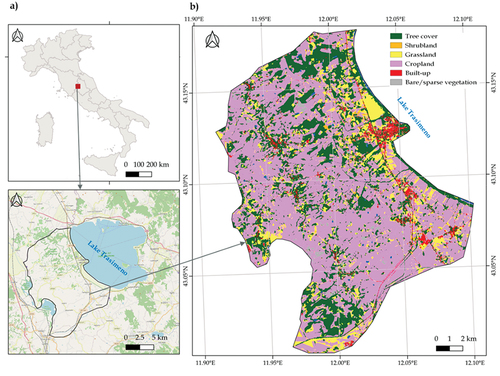
The study area is 154 Km², located around the Trasimeno Lake in Central Italy’s Umbria region [43°06′ N, 12°07′ E] within Castiglione del Lago municipality (Figure 1). This renowned lake, the fourth largest in Italy, is a noteworthy geographical landmark in Umbria’s northwestern region. Covering approximately 120.73 km², it was designated as a regional nature reserve in March 1995, highlighting its ecological importance (Tassi and Vizzari 2020). Notably, the lake’s ecosystem is a precious supplier of varied flora and fauna, offering exceptional environmental value to the surrounding area. Hence, tourism, agriculture, and livestock farming benefit significantly from this location since 70% of its catchment area is surrounded by arable land. The selected area is characterized by a complex landscape mosaic whose agricultural component mainly comprises five crop classes: autumn-winter cereals, corn, sunflower, fava beans, and legume meadows.

Figure 1. Study area location in Italy, Umbria (a), and the 2020 ESA world Cover Map for the same area (b).

2.2. Common Agricultural Policy (CAP) data

In this study, we used IACS tabular crop data for the study area, extracted from farmers’ annual declarations in 2017. Each crop field was specified on a cadastral basis, indicating all the parts of cadastral parcels included in each field. To address the frequent mismatch between actual agricultural fields and cadastral parcels, we selected only those parcels that were at least 90% covered by a single crop and had an area greater than one hectare. This dataset was joined in QGIS to cadastral parcels in shapefile format. Parcels were sampled randomly using points with a minimum distance of 50 meters. This procedure generated an initial ground-sample dataset of 3039 points linked to the crop types derived from farmers’ declarations.

2.3. Satellite data

To produce crop maps, this study employed multi-temporal data collected from both Sentinel-1 (A and B) and Sentinel-2 (A and B) through the GEE Platform from 1 October 2016, to 30 September 2017. Table 1 illustrates the characteristics of the remote sensing dataset employed.

Table 1. Remote sensing datasets used characteristics.

Code	Sensor	Data type	Resolution (m)	Selected Bands	Number of Selected Bands	Processing level
S1	Sentinel-1	Radar (SAR)	10	VV, VH	2	Thermal noise removed, radiometric calibrated, ortho-corrected images
S2	Sentinel-2	Optical	10	B2, B3, B4, B8, B11	5	atmospherically corrected, ortho-corrected, surface reflectance images

The two S1 satellites (A and B), launched by the European Space Agency, provide data using a dual-polarization C-band Synthetic Aperture Radar (SAR) sensor with a spatial resolution of 10, 25, or 40 m and a temporal resolution of 6 days. In GEE, the S1 Toolbox is used to pre-process the Ground Range Detected (GRD) scenes (thermal noise removal, radiometric calibration, terrain correction) to produce calibrated, ortho-corrected images.

On the other hand, the multi-spectral sensor (MSI) on board the two S2 satellites (A and B) detects 13 spectral bands with spatial resolutions of 10, 20, and 60 m and an average temporal resolution of four days. GEE retrieves S2 data from Copernicus Data Hub in two processing levels: L1C for ortho-rectified top-of-atmosphere reflectance and L2A for ortho-rectified, atmospherically corrected, and surface reflectance. At the L2A level, there are three quality assessment (QA) bands, including the bitmask band (QA60) containing cloud mask data.

2.4. Methodology

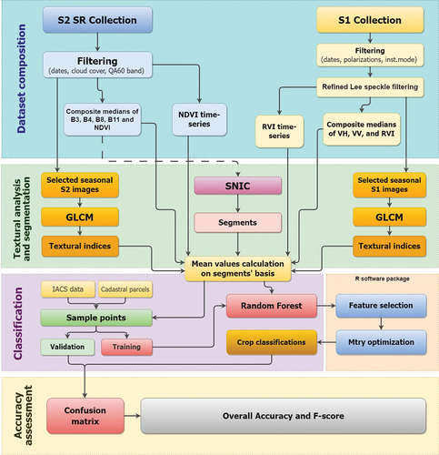
In this research, a comparative analysis was performed across three hierarchical levels of crop classification, ranging from three to seven classes. This was achieved by integrating the OB approach and the Random Forest algorithm, which were applied by combining S1 and S2 datasets, as outlined in Table 1. The methodological workflow is based on four main steps, as illustrated in Figure 2: a) feature dataset composition; b) GLCM textural analysis and segmentation; (c) crop classification; and (d) accuracy assessment. The initial step involved collecting available S2 and S1 images within the selected period and research area. The second step included performing textural analysis using the Gray-Level Co-occurrence Matrix (GLCM) approach, conducting image segmentation with Simple Non-Iterative Clustering (SNIC), and combining data to establish the ultimate feature dataset for crop classification. The third stage contained conducting Random Forest (RF) classifications on the objects’ basis. This includes using a subset of the sample points to train the classifiers and classifying the dataset combinations produced in earlier steps. The fourth step evaluated classification precision using a confusion matrix built by applying the previous step’s RF classifiers to a validation subset of sample points. All these steps were developed in GEE, except for the feature selection and variable per split tuning of RF, which were implemented in the R statistical software (R Development Core Team 2020).

Figure 2. Research methodological workflow.

2.4.1. Dataset composition

S2 dataset composition started by building a filtered and cloud-masked collection of S2 L2A images covering the study area. Considering the available IACS data, we selected the time interval from 1 October 2016 to 30 September 2017 as our interest period. To ensure optimal clarity and reduce the cloud’s impact on image data, we set a threshold of 10% cloudiness for the satellite image selection. This choice was motivated by its proven efficacy and consistency in various research contexts, as demonstrated by several studies (e.g. Meraner et al. 2020). It’s worth noting that the S2 L2A collection in GEE has been available since 28 March 2017, resulting in an initial filtered S2 collection of 20 images (Figure 3). Cloud cover masking was performed using the QA60 band supplied in S2 L2A images and selecting bits 10 and 11 to filter clouds and cirrus, respectively (Baetens, Desjardins, and Hagolle 2019). Vegetation indices, such as the NDVI (Normalized Difference Vegetation Index) (Table 2), are often used to monitor crop vigor and map changes in land cover (Lunetta et al. 2006; Woodcock, Macomber, and Kumar 2010). They have been shown to improve classification accuracy significantly when used for land cover classification (Singh et al. 2016). In this research, NDVI was calculated for each S2 image.

Figure 3. Dates of Sentinel-1 and Sentinel-2 images composing the initial data collection.

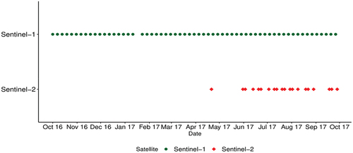
Table 2. Spectral indices formulas used in this study.

Index	Formula	Author
NDVI	$\frac{\mathrm{NIR}-\mathrm{Red}}{\mathrm{NIR}+\mathrm{Red}}$	Rouse et al. (1973)
RVI	$\frac{4{\sigma }^{\text{0}}\text{VH}}{{\sigma }^{\text{0}}\text{VV+}{\sigma }^{\text{0}}\text{VH}}$	Kim and Van Zyl (2009), Trudel et al. (2012)

To compose the S1 dataset, we applied a filter based on the same region and period of interest, selecting the orbit (descending), the instrument mode (IW), and the VV and VH polarizations, with a resolution of 10 meters. The resulting filtered dataset is comprised of 86 images. To enhance data quality, we applied a refined Lee filter, as proposed by Lee et al. (2001), to reduce speckle. This filter was chosen because it better retains polarization information under the influence of speckle elimination (Luo et al. 2021).

Previous research has supported the SAR band ratios’ high explanatory value, particularly during the early phenological crop stages (Veloso et al. 2017; Vergni et al. 2021). Thus, we calculated a modified version of the Radar Vegetation Index (RVI) proposed by Kim and van Zyl (2009) (Table 2). The original quad-pol RVI was modified for dual-pol SAR data by Trudel et al. (2012) based on the assumption that $\mathit{\sigma }{{ }^0}_{\mathit{VH}}$ ≈ $\mathit{\sigma }{{ }^0}_{\mathit{VV}}$. Some studies have already used this alternative formulation for crop monitoring using S1 dual-pol data (Holtgrave et al. 2020; Nasirzadehdizaji et al. 2019).

Using NDVI and RVI, we built a double time-series dataset on a 10-day basis, covering the period of interest. The 10-day time interval was successfully adopted in a previous study aimed at an RF OB crop classification using the S1 time series in central Heilongjiang Province, China (Luo et al. 2021). Besides, two other time sub-periods were defined for data composition, one from December 1 to May 30 (the first period corresponds to the winter-spring season) and the other from June 1 to September 30 (the second period corresponds to the summer season). We used these reference periods to calculate additional median composite spectral bands and indices from S1 and S2 images. Median composite images have proven effective for land cover and crop classification (Hu et al. 2022). This step increased the available information and potentially improved the algorithm’s discretization capacity.

2.4.2. Textural analysis and segmentation

The GLCM algorithm performs by computing a matrix that describes the joint occurrence of pairs of gray levels in an image (Haralick, Shanmugam, and Dinstein 1973). The algorithm requires an 8-bit (gray-level) image as input in GEE. We applied the GLCM to single-date, S2 images, and S1 indices to reduce the band composition procedures’ smoothing effect and potentially obtain more effective textural information. Two representative images of crop cycles were identified within the S2 time series (May 15 for spring and August 31 for summer). As already done in previous studies (Tassi and Vizzari 2020; Tassi et al. 2021), the S2 gray-level image was generated by combining NIR, Red, and Green bands linearly (Formula (1)(1) $\left(0.3\times \mathrm{NIR}\right)+\left(0.59\times \mathrm{RED}\right)+\left(0.11\times \mathrm{GREEN}\right)$(1) ).

(1) $\left(0.3\times \mathrm{NIR}\right)+\left(0.59\times \mathrm{RED}\right)+\left(0.11\times \mathrm{GREEN}\right)$(1)

Similarly, to derive representative textures from the S1 data, we selected two representative RVI images (May 5 for spring and August 21 for summer). Before the GLCM application, as requested in GEE, the S2 and S1 images were rescaled in the 0–255 range (8-bit resolution). In this step, we used the 2nd and 98th percentiles to perform a histogram equalization and improve the textural analysis. After various experiments, the window size for textural analysis was set at 2 pixels. Nine GLCM indices calculated in GEE were selected (Table 3). Moreover, Table 4 summarizes the bands and indices comprising the base feature dataset obtained from the map composition process described above.

Table 3. Textural indices calculated using the GLCM (Gray-Level Co-occurrence Matrix), their description, and the code used in this research.

GLCM code	Textural index description	Code
ASM	Angular Second Moment: measures the number of repeated pairs in the image	T1
CONTR	Contrast: measures the local contrast of an image	T2
CORR	Correlation: measures the correlation between pairs of pixels in the image	T3
VAR	Variance: measures how spread out the distribution of gray-levels is in the image	T4
IDM	Inverse Difference Moment: measures the homogeneity of the image	T5
SAVG	Sum Average: measures the mean of the gray level sum distribution of the image	T6
SVAR	Sum Variance: measures the dispersion (regarding the mean) of the gray-level sum distribution of the image	T7
SENT	Sum Entropy: measures the randomness of the gray-level sum distribution of the image	T8
ENT	Entropy: measures the randomness of the gray-levels distribution of the image	T9

Table 4. Spectral bands, spectral indices, and textural indices included in the base feature dataset.

Satellite	Bands and indices	Number of bands	Codes
Sentinel-1 (S1)	RVI time series	27	RVI_N
	Median composites of VV, VH, and RVI	6	VV_w, VH_w, RVI_w, VV_s, VH_s, and RVI_s
	Textural indices	18	S1wT1 to S1wT9 and S1sT9 to S1sT9
Sentinel-2 (S2)	NDVI time series	12	NDVI_N
	Median composites of B2, B3, B4, B8, B11 and NDVI	12	B2_w, B3_w, B4_w, B8_w, B11_w, NDVI_w, B2_s, B3_s, B4_s, B8_s, B11_s, and NDVI_s
	Textural indices	18	S2wT1 to S2wT9 and S2sT1 to S2sT9
Total		93

Suffixes “w” and “s” indicate the first and second periods, respectively. The suffix “N” represents the average day of the year in the reference period. The codes for textural indices can be found in Table 3.

The Simple Non-Iterative Clustering (SNIC) algorithm is a popular superpixel segmentation method applied to various image processing tasks, including remote sensing imagery (Luo et al. 2021; Tian 2019). This segmentation method involves grouping pixels with similar spectral and spatial properties into cohesive regions or objects, thereby allowing the extraction of valuable information from the imagery (Yang et al. 2021). In GEE, identifying spatial clusters (objects) through SNIC requires configuring four parameters: compactness, connectivity, neighborhood size, and seed spacing. The result is a multi-band raster, including the objects and other layers containing the input image’s mean band values. In this research, SNIC analysis was performed on an S2 median composite dataset (10 meters), based on all the S2 available images, as in previous research (Tassi and Vizzari 2020; Vizzari 2022). After many trials and visual analysis of SNIC outputs, the initial four parameters were set to 1, 8, 128, and 10. A “reduce connected component” step is applied to calculate the average values of the multispectral-textural bands on an object basis to generate the feature dataset for the subsequent classification.

2.4.3. Random forest crop classification

This step defines a three-level crop classification, provides a brief overview of Random Forest (RF) algorithm classification, and performs RF feature selection and variable-per-split tuning.

The main crop classes in the IACS dataset were aggregated into a three-level crop classification based on total area and field numerosity (Table 5). The more detailed classification level was also defined to verify the potentiality of separating crops with similar growth cycles and spectral-textural characteristics, such as wheat vs. barley and maize vs. sorghum.

Table 5. Crop classification levels defined in the study.

Level 1 (L1)		Level 2 (L2)		Level 3 (L3)
Code	Crop class	Code	Crop class	Code	Crop class
0	Winter crops	0	Winter cereals	0	Wheat
				1	Barley
		1	Grain legumes	2	Grain legumes
1	Warm-season crops	2	Warm-season cereals	3	Maize
				4	Sorghum
		3	Sunflower	5	Sunflower
2	Forage crops	4	Forage crops	6	Forage crops

The Random Forest (RF) algorithm, developed by Breiman (2002), is a powerful non-parametric machine learning classifier that is extensively used in land use/land cover and crop classification (Acharki 2022; Acharki et al. 2023; De Luca et al. 2022; Jin et al. 2018; Luo et al. 2021; Oliphant et al. 2019; Su and Zhang 2021). Bootstrap aggregation (bagging) is employed by RF to generate multiple decision trees, which are then merged using a majority voting approach to produce more accurate predictions. Its non-parametric nature, along with low generalization errors and robustness against noise, confirms its versatility in land classification tasks. Moreover, RF’s ability to manage high-dimensional remote sensing data and identify critical variables contributes to its widespread recognition.

Selecting appropriate features is an essential step in building an RF model to improve accuracy, computational efficiency, and reduce overfitting (Puissant, Rougiera, and Stumpf 2014). The Boruta algorithm, a prominent method for this purpose (Degenhardt, Seifert, and Szymczak 2019), compares each feature’s importance in the original dataset to its importance when shuffled randomly (Kursa and Rudnicki 2010). Thus, predictor variables are tested against random shadow variables in multiple runs of RF using statistical testing to determine their significance. If a feature is statistically significant, it is labeled “confirmed” and considered relevant. Conversely, if a feature is not statistically significant, it is marked as “rejected” and is considered unimportant. The algorithm also identifies “tentative” features, which are not statistically significant but highly correlated with confirmed features. The Boruta algorithm is helpful because it can identify essential features even with highly correlated features, which can be difficult for other feature selection methods. It also provides a measure of statistical significance, which can help researchers determine which features to include in their models. To apply the Boruta algorithm in GEE, we used a “sampleRegion” operation to transfer the features’ values to the sample points of the IACS-derived dataset. The Boruta algorithm was run in the R environment on the resulting 2,480-point dataset containing the three-level classification and all the features derived from the previous steps. For each classification level, the algorithm was applied to select the relevant features for the subsequent classification.

Probst et al. (2019) highlighted that the number of randomly drawn variables per regression tree (“mtry”) is one of the most relevant RF parameters. The “mtry” value affects the RF algorithm’s performance since it is necessary to consider the trade-off between the stability and accuracy of the individual trees (Probst, Wright, and Boulesteix 2019). In GEE, this parameter is called “variablesPerSplit” and, as in most RF applications, is set by default as the feature number’s square root (Acharki, Veettil, and Vizzari 2024). Moreover, in this research, we used the “tuneRF” function available in the R randomForest package (Breiman 2002) to find the optimal “mtry” value as performed in previous remote sensing applications (Mohammadpour, Viegas, and Viegas 2022; Stevens et al. 2015). For crop classification, an RF classifier was trained for each classification level using 70% of the IACS-derived sample points, with the remaining 30% for validation. This 70/30 ratio for randomly obtaining training and validation datasets in RF applications is widely used (e.g. Adelabu, Mutanga, and Adam 2015; Chen et al. 2017; Mueller and Massaron 2023).

The GEE “explain” command output was utilized to build a graph showing the feature importance, based on the Gini impurity index, in each classification. This index reflects the likelihood of misclassification when a specific split is applied, ensuring that the variable leading to the most optimal split is the one where the impurity of the two resulting child nodes is minimized. The Gini impurity index, used as a default in GEE, was chosen for this research as it aligns with the standard criteria in the RF algorithm application and decision tree structure building (Breiman 1996). It is also robust in managing class imbalances, making it optimal for crop classification needs (Deschamps et al. 2012).

To filter out non-cropped areas, we used the 2020 ESA WorldCover map’s cropland class as a mask on the study area (Figure 1). Considering the minimal land cover and land use transformation between 2017 and 2020 in the study area, this layer was considered helpful for this purpose.

2.4.4. Accuracy assessment

The confusion matrix is a broadly used methodology for comparing classification results with ground truth data (Congalton and Green 2010). The matrix was used to calculate specific accuracy indices: Overall Accuracy (OA, Equation (2)(2) $\mathit{OA}=\frac{\mathit{Number}\mathit{of}\mathit{correct}\mathit{predictions}}{\mathit{Total}\mathit{number}\mathit{of}\mathit{predictions}}$(2) ), Producer’s Accuracy (PA, Equation (3)(3) $\mathit{PA}=\frac{\mathit{Number}\mathit{correctly}\mathit{identified}\mathit{in}\mathit{agiven}\mathit{class}}{\mathit{Number}\mathit{actually}\mathit{in}\mathit{that}\mathit{class}}$(3) ), and User’s Accuracy (UA, Equation (4)(4) $\mathit{UA}=\frac{\mathit{Number}\mathit{correctly}\mathit{identified}\mathit{in}\mathit{agiven}\mathit{class}}{\mathit{Number}\mathit{claimed}\mathit{to}\mathit{be}\mathit{in}\mathit{that}\mathit{class}}$(4) ), according to the following formulas:

(2) $\mathit{OA}=\frac{\mathit{Number}\mathit{of}\mathit{correct}\mathit{predictions}}{\mathit{Total}\mathit{number}\mathit{of}\mathit{predictions}}$(2)

(3) $\mathit{PA}=\frac{\mathit{Number}\mathit{correctly}\mathit{identified}\mathit{in}\mathit{agiven}\mathit{class}}{\mathit{Number}\mathit{actually}\mathit{in}\mathit{that}\mathit{class}}$(3)

(4) $\mathit{UA}=\frac{\mathit{Number}\mathit{correctly}\mathit{identified}\mathit{in}\mathit{agiven}\mathit{class}}{\mathit{Number}\mathit{claimed}\mathit{to}\mathit{be}\mathit{in}\mathit{that}\mathit{class}}$(4)

The OA is typically represented as a percentage, where 100% signifies that all reference sites were accurately classified. On the other hand, the F-score is a comprehensive measure of accuracy that considers both sensitivity and specificity, providing a more reliable assessment of algorithm performance at the class level (Sokolova, Japkowicz, and Szpakowicz 2006). It is calculated by a harmonic mean of PA and UA (Equation (5)(5) $\mathit{F}\text{-}\mathit{score}=2\times \frac{\mathit{PA}\times \mathit{UA}}{\mathit{PA}+\mathit{UA}}$(5) ). The final accuracy assessment of the three-level classification was based on the OA and the F-scores calculated at the crop class level.

(5) $\mathit{F}\text{-}\mathit{score}=2\times \frac{\mathit{PA}\times \mathit{UA}}{\mathit{PA}+\mathit{UA}}$(5)

3. Results

3.1. Spectral indices analysis

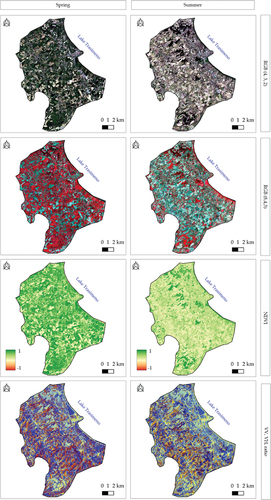
Some image composites and indices for the study area are shown in Figure 4. The optical images (RGB and NDVI composites) clearly show the development of vegetation during spring due to the higher rainwater availability. At the same time, the same images show the bare soils during summer in many parts of the study area. Furthermore, they demonstrate the presence of vegetation in the irrigated portions of the area or the sparse, small woods. The SAR composite images confirm the described seasonality and highlight a high crop spatial variability, which is not as less evident in the optical images.

Figure 4. RGB, near-infrared, NDVI, and SAR median image composites for spring and summer. The SAR composites are obtained using the VV, VH, and their ratio median in the RGB bands.

3.2. Feature selection and importance analysis

The analysis based on Boruta’s algorithm revealed that most features were significant, except for certain textural features listed in Table 6. Notably, the selection process of crucial GLCM features has shown a variable range of 3 to 7 significant variables required for precise crop classification. It is worth noting that Inverse Difference Moment (T5) demonstrates consistency across all levels, satellites, and images, highlighting its ongoing importance in crop classification, irrespective of these variables. Additionally, for S2, Contrast (T2) consistently proves important across all levels, while for S1, Angular Second Moment (T1) holds the highest level of importance.

Table 6. Textural indices selected by Boruta’s algorithm.

Level	Satellite	Image	Codes
L1	S1	Spring, Summer	T1, T5, T9
	S2	Spring, Summer	T2, T5, T7
L2	S1	Spring, Summer	T1, T2, T5, T9
	S2	Spring	T2, T4, T5, T6, T7, T8
		Summer	T2, T4, T5, T7, T8
L3	S1	Spring, Summer	T1, T3, T5, T6, T9
	S2	Spring, Summer	T2, T3, T4, T5, T6, T7, T8

L1: level 1; L2: level 2; L3: level 3; S1: Sentinel-1; S2: Sentinel-2; Textural code descriptions are reported in Table 4.

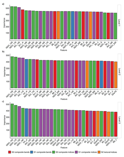
It is noteworthy that the most effective number of variables per split (“mtry”) for each of the three classification levels was identified via the “tuneRF” function in R. Consequently, the settings for L1, L2, and L3 were determined to be 6, 8, and 12, respectively. Furthermore, Figure 4 illustrates the features’ importance in the final RF classification in GEE, quantified by the Gini impurity index, suggested as the optimal measure of variable importance (Menze et al. 2009).

Figure 5 illustrates the relative importance of the top 30 input features in the RF crop classification across the three hierarchical levels. From Figure 5, it is evident that the NDVI and RVI time series provide the most important information for crop discrimination for all three classification levels. As expected, the most relevant information comes from the May to September period. Specifically, the most relevant features across all three classifications include the average NDVI of the first and last decades of June (central DOY 156 and 176) and the average RVI of the central decade of May (central DOY 136). Additionally, certain composite bands and indices, identified distinctly for each classification level, contribute significantly to the classification process. For instance, for Level 1 (L1), B11_w, B8_w, B8_s, B3_s, and B4_s are among the most relevant. For Level 2 (L2), VH_w, B11_w, B8_s, NDVI_w, B3_s, B8_w, VH_s, B3_w, B11_s are identified as the most important. For Level 3 (L3),VH_w, NDVI_w, B8_w, B4_s, B11_w, B3_w, B8_s are highlighted as the most relevant features. The aforementioned features are vital in distinguishing diverse crop types at their respective hierarchical levels. Interestingly, only Sum Average (T6, which measures the average sum of the distances between pixel pairs in the image with a particular combination of gray-level values) from S2, emerges as a consistently significant textural feature in all three classifications. In contrast, although not rejected by Boruta’s algorithm, other textural features consistently show less importance in all three classifications and, as those derived from S1, are not included in the top 30 important features.

Figure 5. Importance and typology of the top 30 features selected for the RF crop classifications ((a): level 1; (b): level 2, (c): level 3). See Table 4 for the feature codes’ explanation.

3.3. Accuracy assessment analysis

The RF classifications achieved an overall accuracy of 0.89 for L1, 0.859 for L2, and 0.815 for L3. This demonstrates the RF algorithm’s and selected features’ overall excellent performance. Additionally, Table 7 presents the F-scores for various crop categories at different classification levels (L1, L2, and L3), generated by RF classifications.

Table 7. F-scores obtained for the crop categories at various classification levels (L1: level 1; L2: level 2; L3: level 3).

Code L1	Crop class L1	F-score	Code L2	Crop classes L2	F-score	Code L3	Crop classes L3	F-score
0	Winter crops	0.936	0	Winter cereals	0.916	0	Wheat	0.860
						1	Barley	0.693
			1	Grain legumes	0.768	2	Grain legumes	0.756
1	Warm-season crops	0.844	2	Warm-season cereals	0.786	3	Maize	0.866
						4	Sorghum	0.782
			3	Sunflower	0.813	5	Sunflower	0.870
2	Forage crops	0.77	4	Forage crops	0.804	6	Forage crops	0.810

From Table 7, it was found that within each level, there are variations in RF performance, with some subclasses having higher or lower F-scores. For Level 1, the RF classifier performed best in discriminating winter crops, followed by warm-season crops, and then forage crops. For instance, it excelled in identifying winter crops, achieving an F-score of about 0.94. Likewise, the classification of warm-season crops yielded a relatively high F-score of 0.844, demonstrating the RF algorithm’s effectiveness in distinguishing between crops grown in different seasons. Nevertheless, the classification of forage crops exhibited a moderate performance, with an F-score of 0.77. At Level 2, the RF classifier proves most accurate in identifying subclasses within winter crops, with forage crops and warm-season crops following closely behind. Notably, the RF classifier performed exceptionally well identifying winter cereals within winter crops, with a high F-score of 0.916.

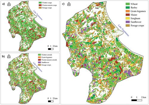
Moreover, the classification of sunflower and forage crops yielded relatively high F-scores of 0.813 and 0.804, respectively, showcasing the algorithm’s effectiveness in differentiating these crop types. Conversely, the classification of grain legumes and warm-season cereals exhibited moderate performance, with F-scores of 0.768 and 0.786, respectively. At the most detailed level (Level 3), the RF classifier performed best in identifying specific crops within their respective classes. Remarkably, sunflower and maize under warm-season cereals have the highest F-score (0.87 and 0.866, respectively), indicating precise classification. The classification of wheat and forage crops also yielded relatively high F-scores of 0.86 and 0.81, respectively. In contrast, the RF algorithm demonstrated moderate performance in classifying grain legumes (0.756) and sorghum (0.723), while barley’s classification had the lowest F-score of 0.693. Figure 6 illustrates the spatial distribution of crop classes across the various classification levels.

Figure 6. RF classification results for the three crop classification levels using S1 and S2 sensors ((a): Level 1; (b): Level 2; (c): Level 3).

4. Discussion

In this research, we implemented a methodology to map crops using the available imagery from Sentinel-2 and Sentinel-1 covering October 2016 to September 2017. Our methodology involved employing an OB approach in Google Earth Engine, including textural analysis and utilizing IACS data for ground-truth training and validation. Unlike a comparable study focused on OB crop classification in GEE using Sentinel-1 time-series (Luo et al. 2021), we developed a more advanced map composition method integrating S1 and S2 time-series data. Moreover, unlike this study, we used a three-level classification containing up to seven crop types, allowing a multi-level classification of the agricultural landscape of the study area. In addition, we applied a textural analysis to improve classification accuracy.

In this work, we used the R statistical software to perform a feature selection step and an optimization of the variable-per-split (“mtry”) parameter. These steps required the preliminary export of the point sample dataset with all the feature values calculated for each point and the subsequent import in the R software. From the operational point of view, these two steps can be performed very quickly and are beneficial for excluding the non-relevant features that may decrease the accuracy of the RF model, slow down the classification process, and automatically find the best mtry value for each classification level. On the other hand, the Boruta algorithm allowed easy identification of the most relevant features for the RF classification. In most cases, the simple analysis of the RF feature importance in GEE as expressed by the importance graph, as performed in other previous studies (Tassi et al. 2021; Vizzari 2022), could be sufficiently efficient for excluding the less relevant features and improving the classification accuracy.

The RVI composite values obtained high relevance in the RF classifications and provided relevant information for crop classification (Figure 5). Notably, these values proved valuable in substituting missing NDVI values in the winter season, addressing the challenge of optical data unavailability in temperate areas during winter and spring due to persistent cloud cover. This finding aligns with Nasirzadehdizaji et al. (2019) research, highlighting that the modified RVI can provide valuable information on crop growth, even with dense cloud cover. In this study, the partial time coverage of the NDVI time series was also determined by the available S2 L2A images in GEE and by the fact that Sentinel-2B became operational in July 2017. In this regard, a more comprehensive S2 time series could help improve classification accuracy results.

This study evaluated the textural features’ utility derived from S1 and S2 data using the GLCM algorithm. Among these GLCM features, the Sum Average (T6) – representing the mean of the gray level sum distribution of the chosen S2 images for spring and summer – emerged as the most relevant. Interestingly, this GLCM feature was identified as a distinctive feature in all three classifications. Conversely, other textural features selected by the Boruta algorithm were considered beneficial but less significant across all three classifications. This evidence confirms the expected difficulty of retrieving relevant textural information for crop discrimination from medium-high resolution imagery like Sentinel-1 and 2 using GLCM. However, the results of the Boruta algorithm’s feature selection and the Sum Average feature’s high relevance for all classification levels suggest that such metrics may improve crop classification accuracy. These results support a previous study that utilized GLCM analysis on S1 data to classify onions and sunflowers (Caballero et al. 2020).

The study’s accuracy for various crops and crop groups shows results that are comparable or superior to previous studies based on IACS georeferenced data (Kyere et al. 2019; Sitokonstantinou et al. 2018). For instance, in Navarra, Spain, Sitokonstantinou et al. (2018) used IACS data and RF classifier training in a parcel-based Sentinel-2 MSI time-series classification approach and achieved an OA of 85.59%. Besides, F-scores obtained for similar growth cycles and spectral-textural characteristics (Table 7), such as wheat (0.86) vs. barley (0.69) and maize (0.87) vs. sorghum (0.78), confirm the proposed approach’s potentiality of separating these similar-structured crops. However, lower accuracies detected for barley and sorghum indicated typical confusion issues between crops with similar spectral and phenological characteristics. In contrast to certain previous studies (Ashourloo et al. 2022; Gerstmann, Möller, and Gläßer 2016) with a specific focus on discriminating wheat and barley, our classification findings exhibited comparatively lower accuracy. For example, Gerstmann et al. (2016), using RapidEye imagery, determined that optimized vegetation indices are more effective for discriminating winter wheat and barley than the well-established vegetation indices, such as NDVI and EVI (OA: 97 vs. 87%). They found that the most significant spectral features for this purpose are the red, red-edge, and near-infrared parts of the spectrum. Similarly, Ashourloo et al. (2022) demonstrated the importance of RedEdge in distinguishing wheat from barley. They obtained excellent results for RF and SVM algorithms (OA: 89 vs. 88%) using Sentinel-2 time series and a phenology-based approach. For future analysis, including the red-edge portion of Sentinel-2 data could be beneficial to investigate the potential improvement in distinguishing closely related cereal crops, like wheat and barley.

Regarding the separation of maize and sorghum, our results are inferior to those obtained in a specific work focused on these two crops based on S2 data, where a very high overall accuracy (98.43%) was obtained using three vegetation indices: the NDVI, the Normalized Difference Water Index (NDWI), and the Structure Insensitive Pigment Index (SIPI) (Soler-Pérez-Salazar et al. 2021). These differences could be due to the low incidence of the sorghum crop in our study area, which gave rise to fewer training points valid to train the RF classifier (Figure 6). Nonetheless, it is noteworthy that our results for both maize and sorghum surpass those obtained in another study (Selvaraj et al. 2021) using Radarsat-2 SAR data and an eigen vector-based classification technique. Selvaraj et al. (2021) reported that the accuracy in discriminating between maize and sorghum crops was approximately 71.6% and 71.4%, respectively.

5. Conclusions

Efficient crop identification and mapping are vital for agriculture, environmental planning, and research. This study investigated the CAP IACS dataset to develop an object-based (OB) approach and Random Forest crop classification using three hierarchical levels within GEE. Our methodology incorporated composite spectral bands, time-series indices, and GLCM textural information from Sentinel-1 and Sentinel-2 data. The achieved overall accuracy (0.89 for Level 1 - including three crop types, 0.86 for Level 2 – including five crop types, and 0.82 for Level 3 – including seven crop types) and the crop maps’ quality indicate a generally excellent performance of the proposed approach. Notably, the results highlighted the reliability of OB approaches in GEE for crop classification and confirmed the importance of integrating multi-source imagery as Sentinel-1 and Sentinel-2. It was also noted that the information derived from the modified Radar Vegetation Index (RVI) was comparably relevant for crop classification with that derived from the traditional NDVI index.

Additionally, the RF model demonstrated superior performance in distinguishing warm-season crops compared to winter cereals. To further evaluate the effectiveness of our proposed approach, future considerations include inter-annual testing for crop classification in GEE with a more extended CAP-derived dataset. Potential challenges in differentiating crops with similar structures, like maize and sorghum, could be mitigated by including the red-edge bands from Sentinel-2, which were not considered in this study. Additional experiments are necessary to assess the advantages of adding GLCM textural analysis to improve crop classification accuracy using Sentinel-1 and Sentinel-2 data. A more comprehensive S2 time series could help improve classification accuracy results.

Disclosure statement

No potential conflict of interest was reported by the author(s).

Data availability statement

All remote sensed data used in the research are openly available in the EU Copernicus archives (https://scihub.copernicus.eu/) and within Google Earth Engine (GEE). IACS data was provided for research purposes by the local Environmental Protection Agency. The GEE codes developed in this research are available upon any reasonable request by emailing the authors.

Additional information

Notes on contributors

Marco Vizzari

Marco Vizzari is an Associate Professor at the University of Perugia (Italy). His expertise spans rural landscape analysis and modeling, land cover classification, design and analysis of rural buildings, spatial multicriteria analysis, ecological networks, ecosystem services analysis and mapping, land survey, as well as precision agriculture. He contributed to this research with conceptualization, supervision, data collection, coding, analysis, writing, and editing.

Giacomo Lesti

Giacomo Lesti earned a Master’s degree in Agricultural Sciences and Technologies from the University of Perugia with summa cum laude. His thesis focused on the classification of agricultural crops using remote sensing in Google Earth Engine. He contributed to this research with coding, analysis, and writing.

Siham Acharki

Siham Acharki is an Engineer-Doctor from Abdelmalek Essaadi University (Morocco), specializing in remote sensing and environment. Her research interests focus on agricultural land use mapping and monitoring, LULC spatiotemporal analysis, and modeling techniques. She is also intrigued by the study of hydro-meteorological processes and climate change’s impact on water resources. She contributed to this research with coding, visualization, writing, and editing.

References

- Acharki, S. 2022. “PlanetScope Contributions Compared to Sentinel-2, and Landsat-8 for LULC Mapping. Remote Sens.” Remote Sensing Applications: Society & Environment 27:100774. https://doi.org/10.1016/j.rsase.2022.100774.
- Acharki, S., P. Frison, B. K. Veettil, Q. B. Pham, S. Singh Kumar, M. Amharref, and A. S. Bernoussi. 2023. “Land Cover and Crop Types Mapping Using Different Spatial Resolution Imagery in a Mediterranean Irrigated Area.” Environmental Monitoring and Assessment 195 (11): 1–20. https://doi.org/10.1007/s10661-023-11877-4.
- Acharki, S., B. K. Veettil, and M. Vizzari. 2024. “Plastic-Covered Greenhouses Mapping in Morocco with Google Earth Engine: Comparing Sentinel-2 and Landsat-8 Data Using Pixel-And Object-Based Methods.” Remote Sensing Applications: Society & Environment 34:101158. https://doi.org/10.1016/j.rsase.2024.101158.
- Adelabu, S., O. Mutanga, and E. Adam. 2015. “Testing the Reliability and Stability of the Internal Accuracy Assessment of Random Forest for Classifying Tree Defoliation Levels Using Different Validation Methods.” Geocarto International 30 (7): 810–821. https://doi.org/10.1080/10106049.2014.997303.
- Aguilar, M. A., A. Vallario, F. J. Aguilar, A. G. Lorca, and C. Parente. 2015. “Object-Based Greenhouse Horticultural Crop Identification from Multi-Temporal Satellite Imagery: A Case Study in Almeria, Spain.” Remote Sensing 7 (6): 7378–7401. https://doi.org/10.3390/RS70607378.
- Ashourloo, D., H. Nematollahi, A. Huete, H. Aghighi, M. Azadbakht, H. S. Shahrabi, and S. Goodarzdashti. 2022. “A New Phenology-Based Method for Mapping Wheat and Barley Using Time-Series of Sentinel-2 Images.” Remote Sensing of Environment 280:113206. https://doi.org/10.1016/J.RSE.2022.113206.
- Baetens, L., C. Desjardins, and O. Hagolle. 2019. “Validation of Copernicus Sentinel-2 Cloud Masks Obtained from MAJA, Sen2Cor, and FMask Processors Using Reference Cloud Masks Generated with a Supervised Active Learning Procedure.” Remote Sensing 11 (4): 433. https://doi.org/10.3390/rs11040433.
- Bahrami, H., H. McNairn, M. Mahdianpari, and S. Homayouni. 2022. “A Meta-Analysis of Remote Sensing Technologies and Methodologies for Crop Characterization.” Remote Sensing 14 (22): 5633–5647. https://doi.org/10.3390/rs14225633.
- Breiman, L. 1996. “Technical Note: Some Properties of Splitting Criteria.” Machine Learning 24 (1): 41–47. https://doi.org/10.1007/BF00117831.
- Breiman, L., 2002. “Manual on Setting Up, Using, and Understanding Random Forests V3. 1, Technical Report.” Berkeley, USA.
- Caballero, G. R., G. Platzeck, A. Pezzola, A. Casella, C. Winschel, S. S. Silva, E. Ludueña, N. Pasqualotto, and J. Delegido. 2020. “Assessment of Multi-Date Sentinel-1 Polarizations and GLCM Texture Features Capacity for Onion and Sunflower Classification in an Irrigated Valley: An Object Level Approach.” Agronomy 10 (6): 845 10, 845. https://doi.org/10.3390/AGRONOMY10060845.
- Chen, W., X. Xie, J. Wang, B. Pradhan, H. Hong, D. T. Bui, Z. Duan, and J. Ma. 2017. “A Comparative Study of Logistic Model Tree, Random Forest, and Classification and Regression Tree Models for Spatial Prediction of Landslide Susceptibility.” Catena 151:147–160. https://doi.org/10.1016/j.catena.2016.11.032.
- Clemente, J. P., G. Fontanelli, G. G. Ovando, Y. L. B. Roa, A. Lapini, and E. Santi, 2020. “Google Earth Engine: Application of Algorithms for Remote Sensing of Crops in Tuscany (Italy).” In 2020 IEEE Latin American GRSS & ISPRS Remote Sensing Conference (LAGIRS), 195–200. Santiago, Chile: IEEE. https://doi.org/10.1109/lagirs48042.2020.9165561.
- Congalton, R. G., and K. Green. 2010. Assessing the Accuracy of Remotely Sensed Data: Principles and Practices, the Photogrammetric Record, Mapping Science Series. Boca Raton: CRC Press. https://doi.org/10.1201/9780429052729.
- Degenhardt, F., S. Seifert, and S. Szymczak. 2019. “Evaluation of Variable Selection Methods for Random Forests and Omics Data Sets.” Briefings in Bioinformatics 20 (2): 492–503. https://doi.org/10.1093/bib/bbx124.
- De Luca, G., J. M. N. Silva, S. Di Fazio, and S. Modica. 2022. “Integrated Use of Sentinel-1 and Sentinel-2 Data and Open-Source Machine Learning Algorithms for Land Cover Mapping in a Mediterranean Region.” European Journal of Remote Sensing 55 (1): 52–70. https://doi.org/10.1080/22797254.2021.2018667.
- Deschamps, B., H. McNairn, J. Shang, and X. Jiao. 2012. “Towards Operational Radar-Only Crop Type Classification: Comparison of a Traditional Decision Tree with a Random Forest Classifier.” Canadian Journal of Remote Sensing 38 (1): 60–68. https://doi.org/10.5589/m12-012.
- Gerstmann, H., M. Möller, and C. Gläßer. 2016. “Optimization of Spectral Indices and Long-Term Separability Analysis for Classification of Cereal Crops Using Multi-Spectral RapidEye Imagery.” International Journal of Applied Earth Observation and Geoinformation 52:115–125. https://doi.org/10.1016/j.jag.2016.06.001.
- Gorelick, N., M. Hancher, M. Dixon, S. Ilyushchenko, D. Thau, and R. Moore. 2017. “Remote Sensing of Environment Google Earth Engine: Planetary-Scale Geospatial Analysis for Everyone.” Remote Sensing of Environment 202:18–27. https://doi.org/10.1016/j.rse.2017.06.031.
- Haralick, R. M., I. Shanmugam, and K. Dinstein. 1973. “Textural Features for Image Classification.” IEEE Transactions on Systems, Man, and Cybernetics SMC-3 (6): 610–621. https://doi.org/10.1109/TSMC.1973.4309314.
- Holtgrave, A. K., N. Röder, A. Ackermann, S. Erasmi, and B. Kleinschmit. 2020. “Comparing Sentinel-1 and -2 Data and Indices for Agricultural Land Use Monitoring.” Remote Sensing 12 (18): 2919. https://doi.org/10.3390/RS12182919.
- Hu, Y., H. Zeng, F. Tian, M. Zhang, B. Wu, S. Gilliams, S. Li, Y. Li, Y. Lu, and H. Yang. 2022. “An Interannual Transfer Learning Approach for Crop Classification in the Hetao Irrigation District, China.” Remote Sensing 14 (5): 1208. https://doi.org/10.3390/rs14051208.
- Jin, Y., X. Liu, Y. Chen, and X. Liang. 2018. “Land-Cover Mapping Using Random Forest Classification and Incorporating NDVI Time-Series and Texture: A Case Study of Central Shandong.” International Journal of Remote Sensing 39 (23): 8703–8723. https://doi.org/10.1080/01431161.2018.1490976.
- Kim, Y., and J. J. Van Zyl. 2009. “A time-series approach to estimate soil moisture using polarimetric radar data.” IEEE Transactions on Geoscience and Remote Sensing: A Publication of the IEEE Geoscience and Remote Sensing Society 47 (8): 2519–2527. https://doi.org/10.1109/TGRS.2009.2014944.
- Kursa, M. B., and W. R. Rudnicki. 2010. “Feature Selection with the Boruta Package.” Journal of Statistical Software 36 (11): 1–13. https://doi.org/10.18637/jss.v036.i11.
- Kyere, I., T. Astor, R. Graß, and M. Wachendorf. 2019. “Multi-Temporal Agricultural Land-Cover Mapping Using Single-Year and Multi-Year Models Based on Landsat Imagery and IACS Data.” Agronomy 9 (6): 309. https://doi.org/10.3390/agronomy9060309.
- Lee, J. S., M. R. Grunes, and E. Pottier. 2001. “Quantitative Comparison of Classification Capability: Fully Polarimetric versus Dual and Single-Polarization SAR.” IEEE Transactions on Geoscience and Remote Sensing: A Publication of the IEEE Geoscience and Remote Sensing Society 39 (11): 2343–2351. https://doi.org/10.1109/36.964970.
- Li, Q., C. Wang, B. Zhang, and L. Lu. 2015. “Object-Based Crop Classification with Landsat-MODIS Enhanced Time-Series Data.” Remote Sensing 7 (12): 16091–16107. https://doi.org/10.3390/RS71215820.
- Lunetta, R. S., J. F. Knight, J. Ediriwickrema, J. G. Lyon, and L. D. Worthy. 2006. “Land-Cover Change Detection Using Multi-Temporal MODIS NDVI Data.” Remote Sensing of Environment 105 (2): 142–154. https://doi.org/10.1016/j.rse.2006.06.018.
- Luo, C., B. Qi, H. Liu, D. Guo, L. Lu, Q. Fu, and Y. Shao. 2021. “Using Time Series Sentinel-1 Images for Object-Oriented Crop Classification in Google Earth Engine.” Remote Sensing 13 (4): 561. https://doi.org/10.3390/RS13040561.
- Menze, B. H., B. M. Kelm, R. Masuch, U. Himmelreich, P. Bachert, W. Petrich, and F. A. Hamprecht. 2009. “A Comparison of Random Forest and Its Gini Importance with Standard Chemometric Methods for the Feature Selection and Classification of Spectral Data.” BMC Bioinformatics 10 (1): 1–16. https://doi.org/10.1186/1471-2105-10-213.
- Meraner, A., P. Ebel, X. X. Zhu, and M. Schmitt. 2020. “Cloud Removal in Sentinel-2 Imagery Using a Deep Residual Neural Network and SAR-Optical Data Fusion.” ISPRS Journal of Photogrammetry and Remote Sensing 166:333–346. https://doi.org/10.1016/j.isprsjprs.2020.05.013.
- Modica, G., G. De Luca, G. Messina, and S. Praticò. 2021. “Comparison and Assessment of Different Object-Based Classifications Using Machine Learning Algorithms and UAVs Multispectral Imagery: A Case Study in a Citrus Orchard and an Onion Crop.” European Journal of Remote Sensing 54 (1): 431–460. https://doi.org/10.1080/22797254.2021.1951623.
- Mohammadpour, P., D. X. Viegas, and C. Viegas. 2022. “Vegetation Mapping with Random Forest Using Sentinel 2 and GLCM Texture Feature—A Case Study for Lousã Region, Portugal.” Remote Sensing 14 (18): 4585. https://doi.org/10.3390/rs14184585.
- Mueller, J. P., and L. Massaron 2023. “Training, Validating, and Testing in Machine Learning.” Accessed October 11. https://www.dummies.com/programming/big-data/data-science/training-validating-testing-machine-learning/.
- Nasirzadehdizaji, R., F. B. Sanli, S. Abdikan, Z. Cakir, A. Sekertekin, and M. Ustuner. 2019. “Sensitivity Analysis of Multi-Temporal Sentinel-1 SAR Parameters to Crop Height and Canopy Coverage.” Applied Sciences 9 (4): 655. https://doi.org/10.3390/APP9040655.
- Oliphant, A. J., P. S. Thenkabail, P. Teluguntla, J. Xiong, M. K. Gumma, R. G. Congalton, and K. Yadav. 2019. “Mapping Cropland Extent of Southeast and Northeast Asia Using Multi-Year Time-Series Landsat 30-M Data Using a Random Forest Classifier on the Google Earth Engine Cloud.” International Journal of Applied Earth Observation and Geoinformation 81:110–124. https://doi.org/10.1016/j.jag.2018.11.014.
- Pande, C. B. 2022. “Land Use/Land Cover and Change Detection Mapping in Rahuri Watershed Area (MS), India Using the Google Earth Engine and Machine Learning Approach.” Geocarto International 37 (26): 13860–13880. https://doi.org/10.1080/10106049.2022.2086622.
- Pande, C. B., and K. N. Moharir. 2023. “Application of Hyperspectral Remote Sensing Role in Precision Farming and Sustainable Agriculture Under Climate Change: A Review.” Climate Change Impacts on Natural Resources, Ecosystems and Agricultural Systems 503–520. https://doi.org/10.1007/978-3-031-19059-9_21.
- Probst, P., M. N. Wright, and A. L. Boulesteix. 2019. “Hyperparameters and Tuning Strategies for Random Forest.” Wiley Interdisciplinary Reviews Data Mining and Knowledge Discovery 9 (3): e1301. https://doi.org/10.1002/WIDM.1301.
- Puissant, A., S. Rougiera, and A. Stumpf. 2014. “Object-Oriented Mapping of Urban Trees Using Random Forestclassifiers.” International Journal of Applied Earth Observation and Geoinformation 26:235–245. https://doi.org/10.1016/j.jag.2013.07.002.
- R Development Core Team. 2020. R: A Language and Environment for Statistical Computing. Vienna, Austria: R Foundation for Statistical Computing.
- Rouse, J. W., R. H. Hass, J. A. Schell, and D. W. Deering. 1973. “Monitoring Vegetation Systems in the Great Plains with ERTS.” Third ERTS Symposium NASA 1:309–317.
- Selvaraj, S., H. S. Srivastava, D. Haldar, and P. Chauhan. 2021. “Eigen Vector-Based Classification of Pearl Millet Crop in Presence of Other Similar Structured (Sorghum and Maize) Crops Using Fully Polarimetric Radarsat-2 SAR Data.” Geocarto international 37 (16): 4857–4869. https://doi.org/10.1080/10106049.2021.1903581.
- Shinde, S., C. B. Pande, V. N. Barai, S. D. Gorantiwar, and A. A. Atre. 2023. “Flood Impact and Damage Assessment Based on the Sentitnel-1 SAR Data Using Google Earth Engine.” In Climate Change Impacts on Natural Resources, Ecosystems and Agricultural Systems (pp. 483–502). Springer International Publishing.
- Singh, R. P., N. Singh, S. Singh, and S. Mukherjee. 2016. “Normalized Difference Vegetation Index (NDVI) Based Classification to Assess the Change in Land Use/Land Cover (LULC) in Lower Assam, India.” International Journal of Advanced Remote Sensing and GIS 5 (1): 1963–1970. https://doi.org/10.23953/cloud.ijarsg.74.
- Sitokonstantinou, V., I. Papoutsis, C. Kontoes, A. L. Arnal, A. P. A. Andrés, and J. A. G. Zurbano. 2018. “Scalable Parcel-Based Crop Identification Scheme Using Sentinel-2 Data Time-Series for the Monitoring of the Common Agricultural Policy.” Remote Sensing 10 (6): 911 10, 911. https://doi.org/10.3390/RS10060911.
- Sokolova, M., N. Japkowicz, and S. Szpakowicz, 2006. “Beyond Accuracy, F-Score and ROC: A Family of Discriminant Measures for Performance Evaluation” in: AAAI Workshop - Technical Report. https://doi.org/10.1007/11941439_114
- Soler-Pérez-Salazar, M. J., N. Ortega-García, M. Vaca-Mier, and S. Cram-Hyedric. 2021. “Maize and Sorghum Field Segregation Using Multi-Temporal Sentinel-2 Data in Central Mexico.” Journal of Applied Remote Sensing 15 (2): 024513. https://doi.org/10.1117/1.JRS.15.024513.
- Song, Q., M. Xiang, C. Hovis, Q. Zhou, M. Lu, H. Tang, and W. Wu. 2019. “Object-Based Feature Selection for Crop Classification Using Multi-Temporal High-Resolution Imagery.” International Journal of Remote Sensing 40 (5–6): 2053–2068. https://doi.org/10.1080/01431161.2018.1475779.
- Stevens, F. R., A. E. Gaughan, C. Linard, A. J. Tatem, and L. A. N. Amaral. 2015. “Disaggregating Census Data for Population Mapping Using Random Forests with Remotely-Sensed and Ancillary Data.” Public Library of Science ONE 10 (2): e0107042. https://doi.org/10.1371/JOURNAL.PONE.0107042.
- Su, T., and S. Zhang. 2021. “Object-Based Crop Classification in Hetao Plain Using Random Forest.” Earth Science Informatics 14 (1): 119–131. https://doi.org/10.1007/S12145-020-00531-Z/TABLES/6.
- Tassi, A., D. Gigante, G. Modica, L. Di Martino, and M. Vizzari. 2021. “Pixel- Vs. Object-Based Landsat 8 Data Classification in Google Earth Engine Using Random Forest: The Case Study of Maiella National Park.” Remote Sensing 13 (12): 2299 13, 2299. https://doi.org/10.3390/RS13122299.
- Tassi, A., and M. Vizzari. 2020. “Object-Oriented Lulc Classification in Google Earth Engine Combining Snic, Glcm, and Machine Learning Algorithms.” Remote Sensing 12 (22): 3776. https://doi.org/10.3390/rs12223776.
- Tian, M. 2019. “Assessing the Value of Superpixel Approaches to Delineate Agricultural Parcels.” Master’s thesis, University of Twente.
- Trudel, M., F. Charbonneau, and R. Leconte. 2012. “Using RADARSAT-2 Polarimetric and ENVISAT-ASAR Dual-Polarization Data for Estimating Soil Moisture Over Agricultural Fields, in.” Canadian Journal of Remote Sensing. https://doi.org/10.5589/m12-043.
- Veloso, A., S. Mermoz, A. Bouvet, T. Le Toan, M. Planells, J. F. Dejoux, and E. Ceschia. 2017. “Understanding the Temporal Behavior of Crops Using Sentinel-1 and Sentinel-2-Like Data for Agricultural Applications.” Remote Sensing of Environment 199:415–426. https://doi.org/10.1016/j.rse.2017.07.015.
- Vergni, L., A. Vinci, F. Todisco, F. S. Santaga, and M. Vizzari. 2021. “Comparing Sentinel-1, Sentinel-2, and Landsat-8 Data in the Early Recognition of Irrigated Areas in Central Italy.” Journal of Agricultural Engineering 52 (4): 43–53. https://doi.org/10.4081/JAE.2021.1265.
- Vizzari, M. 2022. “PlanetScope, Sentinel-2, and Sentinel-1 Data Integration for Object-Based Land Cover Classification in Google Earth Engine.” Remote Sensing 14 (11): 2628. https://doi.org/10.3390/rs14112628.
- Warner, T. 2011. “Kernel-Based Texture in Remote Sensing Image Classification.” Geography Compass 5 (10): 781–798. https://doi.org/10.1111/J.1749-8198.2011.00451.X.
- Woodcock, C. E., S. A. Macomber, and L. Kumar, 2010. Vegetation mapping and monitoring. Environmental Modelling with GIS and Remote Sensing. https://doi.org/10.4324/9780203302217_chapter_6
- Xiong, J., P. S. Thenkabail, J. C. Tilton, M. K. Gumma, P. Teluguntla, A. Oliphant, R. G. Congalton, K. Yadav, and N. Gorelick. 2017. “Nominal 30-M Cropland Extent Map of Continental Africa by Integrating Pixel-Based and Object-Based Algorithms Using Sentinel-2 and Landsat-8 Data on Google Earth Engine.” Remote Sensing 9 (10): 1–27. https://doi.org/10.3390/rs9101065.
- Xue, H., X. Xu, Q. Zhu, G. Yang, H. Long, H. Li, X. Yang, et al. 2023. “Object-Oriented Crop Classification Using Time Series Sentinel Images from Google Earth Engine.” Remote Sensing 15 (5): 1353. https://doi.org/10.3390/rs15051353.
- Yang, L., L. Wang, G. A. Abubakar, and J. Huang. 2021. “High‐Resolution Rice Mapping Based on Snic Segmentation and Multi‐Source Remote Sensing Images.” Remote Sensing 13 (6): 1148. https://doi.org/10.3390/rs13061148.