Enhancing outlying growth simulation in urban cellular automata via intelligent extraction-fusion of land suitability and neighborhood effects: a case study of Wuhan, China

ABSTRACT

Urban growth has accelerated significantly in recent decades, categorized into two spatial patterns: adjacent and outlying growth. Traditional Cellular Automata (CA)-based models excel at simulating adjacent growth but exhibit limitations in modeling outlying growth, which can be summarized into two issues: 1) the overestimation of neighborhood effects caused by models’ excessive dependence on neighboring cell states; and 2) the ignorance of spatial heterogeneity in the relative importance of land suitability and neighborhood effects on urban growth. To address these problems, a novel CA model with Separate Extraction and Adaptive Fusion of land suitability and neighborhood effects (SEAF-CA) is proposed. In this model, a dual-path convolution structure is employed to extract spatial features from driving factors and cell states; geographical coordinates of each cell then input into a multilayer perceptron to derive spatially varying weights for feature fusion. Finally, the derived conversion probability is integrated with CA to simulate urban growth. Land use data collected from 2000 to 2020 in Wuhan are selected to evaluate the proposed model. Experimental results illustrate that SEAF-CA outperforms three typical CA models, achieving the closest outlying growth proportion to reality and the highest simulation accuracy. In addition, the source code of SEAF-CA is now available at GitHub (https://github.com/ohXu/SEAF-CA).

KEYWORDS:

• Urban growth
• cellular automata
• deep learning
• outlying growth
• land suitability
• neighborhood effects

1. Introduction

Expeditious urbanization has swept over most countries throughout the world in the past few decades, resulting in urban land now accommodating more than half of the global population (G. Chen et al. 2020; Wang et al. 2022). While urbanization greatly improves the living standards of residents in education, traffic, and economy, etc., it can also have severe negative impacts, including environmental deterioration and resource depletion (Isinkaralar, Isinkaralar, and Yilmaz 2023; Zhao and Sing 2017). Therefore, accurate urban growth simulation is of great necessity for scientific urban planning and sustainable development (Guan et al. 2023; Masoumi and Genderen 2023; Yan et al. 2021).

1.1. Spatial patterns of urban growth

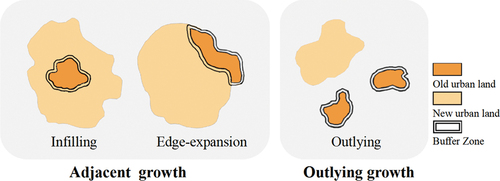
As a complicated dynamic process, urban growth can usually be categorized into three modes according to the spatial patterns of evolution involved: namely, infilling growth, edge expansion, and outlying growth (Clarke, Hoppen, and Gaydos 1997; Southworth and Owens 1993). As shown in Figure 1, infilling growth represents the process in which non-urban areas surrounded by urban areas will be transformed into urban areas, edge expansion refers to outward growth along the edges of existing urban areas, and outlying growth is characterized by the isolation of newly developed urban areas from existing ones. Since both infilling growth and edge expansion can be regarded as an orderly diffusion process of existing urban areas into neighboring areas, they can be collectively conceptualized as adjacent growth (Liu et al. 2014). Adjacent growth is mainly driven by neighborhood interactions; in short, if an area is already urbanized, its adjacent non-urban areas have a high probability of transformation into urban lands. Compared with adjacent growth, outlying growth relies less on neighboring land use states but more on Land Suitability (LS), determined by local resources like flat terrain, adequate water (Feng et al. 2019; He et al. 2018; Wu 2002; Zhai et al. 2020).

Figure 1. Three types of urban growth.

1.2. Issues in existing urban growth simulation

Various simulation models have been developed to model the spatial process of urban growth. Among these models, Cellular Automata (CA)-based models have remained continuously popular due to their simplicity and flexibility (Batty 1998; Clarke and Gaydos 1998; Li and Yeh 2000; Liu et al. 2017). A CA model consists of discrete cells arranged in a grid of specified shape. Each cell updates its state according to the transition rules, typically expressed as a function of LS, neighborhood effects NE, spatial constraints SC, and randomness factors Rand (Dahal and Chow 2015; Fonstad 2006; Yang, Li, and Shi 2008; Zhang et al. 2023). Among the above four components, LS and NE mainly determine the simulation results (Kamusoko and Gamba 2015; Li, Yang, and Liu 2007). Specifically, LS serves as a representation of the urban growth potential estimated by driving factors (i.e. contributing resources), while NE characterizes the impact of neighboring cell states (urban or non-urban) on the development of the central cell.

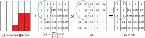
Since LS and NE represent the effects of driving factors and cell states on urban growth respectively, any attempts to characterize the combined impacts of both components must design a suitable fusion strategy between them. Currently, most CA-based models adopt the multiplication strategy to fuse both components for transition probability calculation, i.e. $\mathit{LS}\times \mathit{NE}$ (Feng et al. 2011; Wu et al. 2012; Xu et al. 2022; Zhang and Xia 2022). However, the NE value of most suburban cells is typically extremely low due to the absence of nearby urban cells, resulting in a low $\mathit{LS}\times \mathit{NE}$ value even if the LS value is large. This is exemplified in Figure 2, where the NE values of the cells in the blue ellipse are zero, while the LS values are close to the maximum (i.e. 1). However, the multiplication results remain zero, meaning that sufficient resources for state transformation in these cells are still overlooked. Therefore, the multiplication strategy is inefficient at simulating outlying growth but excels in adjacent growth modeling, and as a result, most of the simulated urban transitions occur in regions adjacent to existing urban areas (Liu et al. 2014).

Figure 2. Illustration of NE, LS and their product.

Some attempts have been made in recent years to address the deficiency of the multiplication strategy in simulating outlying growth. These attempts can be divided into two categories, as outlined below.

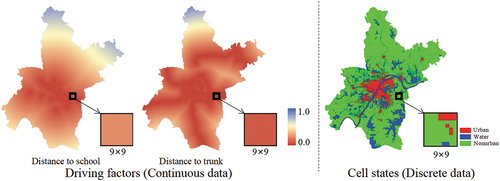
In the first category, both driving factors and cell states are input into one algorithm simultaneously to derive a unified output, which obviates the need for independent calculations of the specific values of LS and NE. For example, Liu et al. (2008) and Cao et al. (2016) established a series of “if-then” rules based on driving factors and cell states. However, these rules typically represent simple cause-and-effect relationships and cannot capture complex interactions among variables. Pal and Ghosh (2017) proposed an end-to-end urban growth prediction framework, but this model suffers from slow convergence speed and low simulation accuracy. Xing et al. (2020) and Qian et al. (2020) organized driving factors and cell states into a 3D data cube that is input into a Convolutional Neural Network (CNN), after which the network output denotes the combined impacts of LS and NE on urban growth. However, as shown in Figure 3, driving factors are typically continuous data with little variation in values within the neighborhood of one given cell, while the states of its neighboring cells are discrete with higher-gradient variations. Due to the sensitivity of CNN to high-gradient variations (Yamashita et al. 2018), combining these two types of data together will result in neighboring cell states contributing excessively to the model’s inference. Thus, these methods are still inefficient for accurately modeling the outlying growth in the simulation.

Figure 3. Differences between driving factors and cell states.

In the second category, other fusion strategies for LS and NE are proposed to reduce the occurrence of zero-value results caused by direct multiplication. Liu et al. (2014) and Liu et al. (2016) removed NE from transition rules for the non-urban cells identified as outlying growth by pre-classification. However, high cumulative errors are inevitable due to the involvement of a complex pre-classification process. Mustafa et al. (2018) added an exponential parameter σ for NE to express its relative importance and used square roots multiplication to fuse LS and $\mathit{N}{E}^{\sigma }$. However, the value of σ substantially influences the simulation results, and extensive repeated experiments are required to find the most suitable value of σ. Furthermore, Feng and Tong (2020) proposed a weighted sum method to fuse LS and NE, widely applied in their subsequent research (Feng et al. 2022; Li et al. 2022; Yan et al. 2021). Notably, in these models, the assigned weights are fixed, despite the fact that the relative importance of LS and NE for urban growth varies from region to region. Therefore, it is necessary to develop a spatially varying weight-assigning scheme to fuse LS and NE.

1.3. Our solution and main contributions

To tackle these issues, a deep learning-based CA model with separate extraction and adaptive fusion of LS/NE (SEAF-CA) is proposed. The model utilizes a parallel dual-path structure to separately extract spatial features from driving factors and cell states, then adaptively assigns spatially varying weights to fuse both features. Taking Wuhan, China as a case study, the model was calibrated with 2000–2010 data and subsequently validated with 2010–2020 data. The results demonstrate that SEAF-CA outperforms other existing models in terms of both the proportion of the simulated outlying growth and simulation accuracy.

The main contributions of this paper can be summarized as follows:

1. A separate extraction module is designed as a dual-path structure to perform parallel convolution on driving factors and cell states. Each path has its own attention distribution through automatic learning of historical growth patterns, which can avoid the overestimation of NE.

2. An adaptive fusion module is proposed to adaptively assign various weights to the spatial features extracted from driving factors and cell states according to geographical coordinates, then fuse both weighted features by means of a full connection layer. This process can characterize the unequal impacts of LS and NE on the central cell.

3. The performance of the proposed model has been evaluated on a real land use dataset. The proposed SEAF-CA outperforms three typical CA models, not only achieving the highest simulation accuracy (with an average increase in the Figure of Merit (FoM) of 1.1%), but also obtaining the proportion of simulated outlying growth closest to reality (with an average reduction in the Mean Expansion Index (MEI) of 8.7).

2. Materials

2.1. Study area

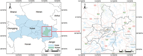
As shown in Figure 4, Wuhan is located in the east-central part of Hubei Province, covering a region of latitude 29°58′–31°22′ N and longitude 113°41′–115°05′ E. Over the past two decades, the urbanized area of Wuhan has experienced a substantial increase, growing from 210 km² in 2000 to 885 km² in 2020. The population of Wuhan has reached 12.32 million by 2020, with 84.31% identified as urban residents. The derived environmental deterioration and resource depletion are threatening the stability of the Yangtze River Economic Belt. Furthermore, the city consists of 13 administrative districts with varying levels of urbanization, which represents strong spatial heterogeneity in the urbanization process. Therefore, Wuhan is selected as the study area to examine the effectiveness of the proposed model.

Figure 4. Location of study area.

2.2. Data sources and preparation

Four public datasets were applied to calibrate and validate the proposed model. The land use data was from Yang and Huang’s (2021) China land cover dataset (CLOD) (irsip.whu.edu.cn/resources/resources_v2.php), with a classification accuracy of 79.31%. The administrative map was obtained from the National Catalogue Service For Geographic Information (www.webmap.cn). The infrastructure datasets were collected from OpenStreetMap (OSM) (www.openstreetmap.org). The Geospatial Data Cloud (www.gscloud.cn) provides Shuttle Radar Topography Mission (SRTM) data for terrain assessment. In the area of Hubei Province, SRTM displays varying accuracy across different terrains, with measurements of 2.6 ± 1.7 m on plains, 2.4 ± 11.3 m on hills, and 1.5 ± 21.3 m on mountains (Hu et al. 2017).

Table 1 details the dependent and independent variables for the proposed model. The land use data in 2000, 2010, and 2020 were reclassified into three categories (urban land, non-urban land, and water), producing three urban pattern maps. The dependent variable represents the change between the two urban pattern maps, where the value of 0 denotes state persistence and 1 denotes state change (Gao et al. 2020). The independent variables include the distance-based variables calculated from the infrastructure datasets using the Euclidean distance tool, Digital Elevation Model (DEM) data and the derived slope data, and the initial urban pattern map. All variables were resampled to 90 m spatial resolution and normalized to [0, 1] to reduce calculation cost and accelerate the simulation process (Li et al. 2022).

Table 1. List of factors in this study.

Category	Variable	Descriptions	Data Source
Response	y	Differences between two urban pattern maps	CLOD (2000, 2010, 2020)
Explanatory	DisMot	Euclidean distance to motorway	OSM (2020)
Explanatory	DisTru	Euclidean distance to trunks	OSM (2020)
Explanatory	DisPri	Euclidean distance to primary roads	OSM (2020)
Explanatory	DisSec	Euclidean distance to secondary roads	OSM (2020)
Explanatory	DisTer	Euclidean distance to tertiary roads	OSM (2020)
Explanatory	DisRai	Euclidean distance to railways	OSM (2020)
Explanatory	DisWat	Euclidean distance to waterways	OSM (2020)
Explanatory	DisBS	Euclidean distance to bus stops	OSM (2020)
Explanatory	DisRS	Euclidean distance to railway stations	OSM (2020)
Explanatory	DisSch	Euclidean distance to schools	OSM (2020)
Explanatory	DEM	Elevation	SRTM (2008)
Explanatory	Slope	Slope derived from elevation	SRTM (2008)
Explanatory	NCS	Urban pattern map	CLOD (2000, 2010)

The selected infrastructure datasets include two categories: transport lines and public facilities. Transport lines connect different regions, promoting cultural, commercial and social exchanges. Numerous studies have identified transport lines as a major driver of urban growth, capable of guiding urban growth through improved accessibility (Kasraian, Maat, and Wee 2019; Kelobonye et al. 2019; Meng et al. 2023). Thus, seven types of transport lines were selected as driving factors in this research, including motorways, trunk roads, primary roads, secondary roads, tertiary roads, railways, and waterways. Public facilities significantly facilitate people’s daily lives and work, leading to that locations closer to public facilities are more likely to convert into built-up areas. Thus, accessibility to public facilities have been frequently selected as driving factors in previous research (Li et al. 2022; Qian et al. 2020; Zhu et al. 2023). In this study, we focus on three common public facilities, i.e. schools, bus stops and railway stations. Furthermore, factors related to topography also affect an area’s suitability for urban growth. Consistent with the research conducted by Liu et al. (2017) and He et al. (2018), elevation and slope are the two indicators employed to characterize geographical conditions in this study.

3. Methods

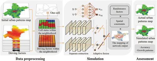
Figure 5 shows the proposed workflow in the SEAF-CA urban growth model, including the following three steps:

1. Data preprocessing. For each non-urban cell, cell states and driving factors within its neighborhood (defined by a certain window size) are obtained.

2. Model simulation. The derived driving factors and cell states are set as the inputs of two CNN-based branches for modeling LS and NE respectively. The geographical coordinate of each cell is used as the input of a Multilayer Perceptron (MLP) to obtain spatially varying weights for LS and NE features. The network output is integrated with spatial constraints and randomness factor to generate the final simulation result.

3. Model assessment. The simulation results are compared with the observed results in terms of accuracy and growth patterns.

Figure 5. Procedure for modeling dynamic urban growth using the SEAF-CA model.

3.1. Separate extraction of LS and NE using a dual-path structure

As stated in Section 1, integrating driving factors and cell states as data cubes and inputting them into a network is inefficient for modeling urban outlying growth. Therefore, SEAF-CA employs a dual-path structure to extract different spatial features from driving factors and cell states.

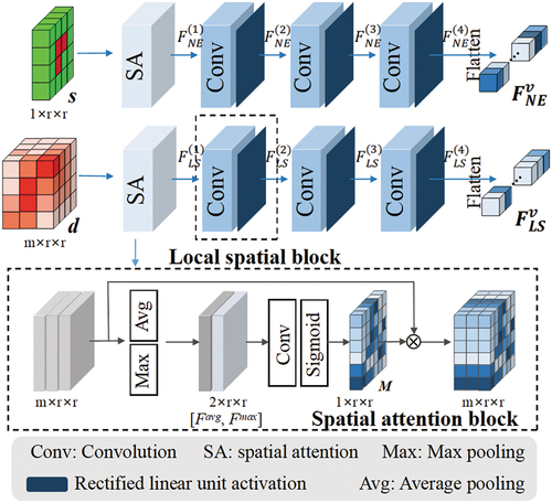
In Figure 6, the proposed dual-path structure includes two parallel branches, where driving factors d∈R^m*r*r and cell states s∈R^1*r*r are input into separate branches. Here, m denotes the number of driving factors, and r denotes the neighborhood size. As shown in Figure 6, each path contains a spatial attention block and three local spatial blocks. Specifically, the spatial attention block aims to characterize the unequal impacts of neighboring cells on the central cell’s growth by assigning various attention coefficients to different spatial locations. The block firstly aggregates features information of the input by using an average pooling layer and a max pooling layer, and generates two 2D maps: $F^{\mathrm{avg}}$ and $F^{\max }$. Both maps are then concatenated to form a simple spatial context descriptor $[F^{\mathrm{avg}};F^{\max }]$ and convolved by a 3 × 3 convolution layer with a sigmoid activation function, producing normalized 2D spatial attention map M. Finally, M is element-wise multiplied with the input to derive spatially weighted features. The specific calculation of the spatial attention block is shown in Equations (1(1) $F_{LS}^{(l)}=\mathit{d}\odot {\sigma }_{\mathit{sig}}(f_{LS}^{3\times 3}([\mathit{AvgPool}(\mathit{d});\mathit{MaxPool}(\mathit{d})]))$(1) –2(2) $F_{NE}^{(l)}=\mathit{s}\odot {\sigma }_{\mathit{sig}}(f_{NE}^{3\times 3}([\mathit{AvgPool}(\mathit{s});\mathit{MaxPool}(\mathit{s})]))$(2) ):

(1) $F_{LS}^{(l)}=\mathit{d}\odot {\sigma }_{\mathit{sig}}(f_{LS}^{3\times 3}([\mathit{AvgPool}(\mathit{d});\mathit{MaxPool}(\mathit{d})]))$(1)

(2) $F_{NE}^{(l)}=\mathit{s}\odot {\sigma }_{\mathit{sig}}(f_{NE}^{3\times 3}([\mathit{AvgPool}(\mathit{s});\mathit{MaxPool}(\mathit{s})]))$(2)

Figure 6. Illustration of separate extraction module.

where $F_{LS}^{(l)}$ and $F_{NE}^{(l)}$ respectively denote the spatially weighted driving factors and cell states; ${\sigma }_{\mathit{sig}}$ denotes the sigmoid function; $f^{3\times 3}$ denotes a convolution operation with the kernel size of 3 × 3, and $\odot$ denotes the Hadamard product.

After the spatial attention block, three local spatial blocks are used to fully extract spatial information by multiple convolution operations. Each block consists of a convolution layer and a Rectified Linear Unit (ReLU) activation layer. The kernel size of these three convolutional layers is 3 × 3, with a channel number of 16. Unlike existing CNN-CA models (He et al. 2018; Xing et al. 2020), the pooling layer is removed in these blocks to reduce the loss of spatial information. The overall operation of the local spatial block can be represented by Equations (3(3) $F_{LS}^{(l+1)}={\sigma }_{\mathrm{ReLU}}(f_{LS}^{3\times 3(l)}(F_{LS}^{(l)})),\mathit{\hspace{0.17em}}\mathit{l}=1,2,3$(3) –4(4) $F_{NE}^{(l+1)}={\sigma }_{\mathrm{ReLU}}(f_{NE}^{3\times 3(l)}(F_{NE}^{(l)})),\mathit{\hspace{0.17em}}\mathit{l}=1,2,3$(4) ):

(3) $F_{LS}^{(l+1)}={\sigma }_{\mathrm{ReLU}}(f_{LS}^{3\times 3(l)}(F_{LS}^{(l)})),\mathit{\hspace{0.17em}}\mathit{l}=1,2,3$(3)

(4) $F_{NE}^{(l+1)}={\sigma }_{\mathrm{ReLU}}(f_{NE}^{3\times 3(l)}(F_{NE}^{(l)})),\mathit{\hspace{0.17em}}\mathit{l}=1,2,3$(4)

where ${\sigma }_{\mathit{ReLU}}$ denotes the ReLU activation function; $f_{LS}^{3\times 3(l)}$ and $f_{NE}^{3\times 3(l)}$ respectively denotes l-th convolution operation in two paths. Finally, both the generated feature maps $f_{LS}^4,f_{NE}^4$ are flattened into one-dimensional feature vectors $f_{LS}^v,f_{NE}^v$ that characterize land suitability and neighborhood effect respectively.

3.2. Adaptive fusion of LS and NE based on spatial location

In typical CA models, all cells are assigned equal weights for LS and NE, which overlooks intricate spatial heterogeneity in their relative importance, i.e. the effects of these two factors on urban growth may vary with the spatial location. Therefore, in the proposed model, geographical coordinates are incorporated to derive adaptive weights w_LS, w_NE for each cell based on their locations.

As shown in Figure 7, the MLP takes the geographical coordinates p of the central cell as input and consists of three units, each of which contains fully connected layers, batch normalization, and activation operations. The three fully connected layers are configured with 16, 16, and 2 neurons, respectively. Next, the Softmax function is applied to ensure that the two weights add up to 1 (i.e. $w_{\mathit{LS}}+w_{\mathit{NE}}=1$). The overall calculation process can be represented by Equations (5(5) $F_{pos}^{(0)}=\mathit{p},\mathit{p}\in R^2$(5) –8(8) $w_{\mathit{NE}}=\frac{exp(F_{pos,2}^{(3)})}{exp(F_{pos,1}^{(3)})+exp(F_{pos,2}^{(3)})},\mathit{\hspace{0.17em}}{F}_{pos}^{(3)}\in R^2$(8) ):

(5) $F_{pos}^{(0)}=\mathit{p},\mathit{p}\in R^2$(5)

(6) $F_{pos}^{(l+1)}={\sigma }_R(\mathit{\phi }(W_{pos}^{(l)}\cdot F_{pos}^{(l)}+b_{pos}^{(l)})),\mathit{\hspace{0.17em}}\mathit{l}=0,1,2$(6)

(7) $w_{\mathit{LS}}=\frac{exp(F_{pos,1}^{(3)})}{exp(F_{pos,1}^{(3)})+exp(F_{pos,2}^{(3)})},\mathit{\hspace{0.17em}}{F}_{pos}^{(3)}\in R^2$(7)

(8) $w_{\mathit{NE}}=\frac{exp(F_{pos,2}^{(3)})}{exp(F_{pos,1}^{(3)})+exp(F_{pos,2}^{(3)})},\mathit{\hspace{0.17em}}{F}_{pos}^{(3)}\in R^2$(8)

where $\mathit{\phi }$ denotes the batch normalization operation, $F_{pos}^{(l+1)}$ denotes the output of the (l +1)-th unit, $W_{pos}^{(l)}$ and $b_{pos}^{(l)}$ denote the learnable parameters in fully connected layers, and $F_{pos,1}^{(3)}$ and $F_{pos,2}^{(3)}$ denote the two outputs of MLP respectively.

Figure 7. Illustration of adaptive fusion module.

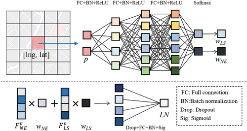
After obtaining adaptive weights, the extracted features in Section 3.1 are merged with both weights, and the resulting weighted features are combined via element-wise addition, leading to a new feature vector $F_{LN}^v$, as shown in Equation (9)(9) $F_{LN}^v=w_{\mathit{LS}}\times F_{LS}^v+w_{\mathit{NE}}\times F_{NE}^v$(9) :

(9) $F_{LN}^v=w_{\mathit{LS}}\times F_{LS}^v+w_{\mathit{NE}}\times F_{NE}^v$(9)

The dropout layer with 0.2 dropout rate is further adopted to address overfitting in the simulation by randomly dropping units from the neural network during training. Finally, a fully connected layer is used to transform the feature vector into a single value, and the sigmoid function is exploited to normalize the output value within the range of [0, 1], as shown in Equation (10)(10) $\mathit{LN}=\frac{1}{1+exp(-({\mathit{W}}_{\mathit{LN}}\cdot F_{LN}^v+b_{\mathit{LN}}))}$(10) :

(10) $\mathit{LN}=\frac{1}{1+exp(-({\mathit{W}}_{\mathit{LN}}\cdot F_{LN}^v+b_{\mathit{LN}}))}$(10)

where $W_{\mathit{LN}}$ and $b_{\mathit{LN}}$ denote the learnable parameters in the fully connected layer. Moreover, LN denotes the combined impact of land suitability and neighborhood effects; the closer the value is to 1, the higher the development potential of the cell.

3.3. Integrating the neural network with cellular automata

The LN output from the extraction-fusion module, which represents the combined impacts of LS and NE, is subsequently input into the CA for urban growth simulation. The complete transition rule of the urban CA model also includes SC and Rand.

SC indicates the constraints of transforming from non-urban land types to urban. In this research, water areas in the initial year are set as restrictive areas (Zhang and Xia 2022), i.e. the cell states within these areas remain unchanged throughout the simulation. As shown in Equation (11)(11) $\mathit{S}{C}_i=\left\{\begin{array}{c}0,S_i^{{\mathit{t}}_{\mathit{initial}}}\mathrm{is}\mathrm{water}\\ 1,\mathrm{otherwise}\end{array}\right.$(11) , $S_i^{{\mathit{t}}_{\mathit{initial}}}$ denotes the land use state of cell i at the initial time, and the constraints can be characterized with a value of 0 or 1, where 1 means no restriction on the development of the cell into urban state and 0 means that the cell is restricted from being developed into urban state.

(11) $\mathit{S}{C}_i=\left\{\begin{array}{c}0,S_i^{{\mathit{t}}_{\mathit{initial}}}\mathrm{is}\mathrm{water}\\ 1,\mathrm{otherwise}\end{array}\right.$(11)

Rand represent uncertainties in the urban growth process, such as natural disasters and subjectivity in decision-making, which could be represented as a stochastic perturbation term (White and Engelen 1993):

(12) $\mathit{Ran}{d}_i=1+(-In{R}_i{)}^a$(12)

where $\mathit{Ran}{d}_i$ is a random interference coefficient on cell i, $R_i$ is a random number between 0 and 1, and a is a parameter used to control the strength of stochastic perturbation. The overall transition probability $P_{Al{l}_i}$ can be generated by Equation (13)(13) $P_{Al{l}_i}=\mathit{L}{N}_i\times \mathit{S}{C}_i\times \mathit{Ran}{d}_i$(13) :

(13) $P_{Al{l}_i}=\mathit{L}{N}_i\times \mathit{S}{C}_i\times \mathit{Ran}{d}_i$(13)

The demand of urban land transition within the given time period has the characteristics of a Markov chain (Moghadam and Helbich 2013). Based on this Markov chain, if the non-urban-to-urban transformation rate in the last time step is represented by $R_{\mathit{n}2\mathit{u}}$, urban growth demand in this time step should be $R_{\mathit{n}2\mathit{u}}\times \mathit{N}$, where N denotes the current number of non-urban cells. Thus, a threshold value P_thd could be calculated as in Equation (14)(14) $P_{\mathit{thd}}=\mathit{sort}(P_{\mathit{All}}{)}_{{\mathit{R}}_{\mathit{n}2\mathit{u}}\times \mathit{N}}$(14) :

(14) $P_{\mathit{thd}}=\mathit{sort}(P_{\mathit{All}}{)}_{{\mathit{R}}_{\mathit{n}2\mathit{u}}\times \mathit{N}}$(14)

where sort() denotes a function that sorts the contents of an array in a descending order. As shown in Equation (15)(15) $S_i^{t+1}=\left\{\begin{array}{c}\mathit{Urban},\mathit{\hspace{0.17em}}{P}_{Al{l}_i}\ge P_{\mathit{thd}}\mathrm{or}{S}_i^t=\mathit{Urban}\\ \mathit{NonUrban},\mathit{\hspace{0.17em}}{P}_{Al{l}_i}<P_{\mathit{thd}}\mathrm{and}{S}_i^t=\mathit{NonUrban}\mathit{\hspace{0.17em}}\end{array}\right.$(15) , by comparing the overall transition probability $P_{Al{l}_i}$ with the threshold $P_{\mathit{thd}}$, the model can determine whether the state of cell i will change at the next time step. If $P_{Al{l}_i}<P_{\mathit{thd}}$, the state of the cell i will remain unchanged; otherwise, the non-urban cell will be converted to an urban land cell.

(15) $S_i^{t+1}=\left\{\begin{array}{c}\mathit{Urban},\mathit{\hspace{0.17em}}{P}_{Al{l}_i}\ge P_{\mathit{thd}}\mathrm{or}{S}_i^t=\mathit{Urban}\\ \mathit{NonUrban},\mathit{\hspace{0.17em}}{P}_{Al{l}_i}<P_{\mathit{thd}}\mathrm{and}{S}_i^t=\mathit{NonUrban}\mathit{\hspace{0.17em}}\end{array}\right.$(15)

4. Results and analysis

4.1. Experimental settings

4.1.1. Experiment implementations

(1) Computing environment

All experiments are conducted on a Linux machine with one Intel Core i7-9700F [email protected] GHz and one NVIDIA RTX 2080Ti GPU. All deep learning models are implemented using an open-source framework, PyTorch (version 1.7.0).

(2) Model calibration and validation

During model calibration, the model parameters are learned based on the land use data in Wuhan city during 2000–2010. The training set is generated by systematic sampling with a sample rate of 5% and a sample prevalence of 1:1, following Zhang and Xia’s settings (2022). Through multiple experiments, the neighborhood size is set to 9; the Adam optimizer with a learning rate of 0.0005 is used to conduct model updating; and the loss function adopted is binary cross-entropy loss. If the loss is not reduced within 10 epochs, the training process is stopped before completing all 100 epochs. During model validation, the learned model is directly applied to simulate urban growth during 2010–2020.

(3) Baselines

In addition to the proposed SEAF-CA model, three existing CA models introduced in the first section and another variant of the proposed model are developed for comparison; for fairness, the CNN components are kept the same.

MUL-CA: Classical constrained CA. This model uses two Convolutional Neural Networks (CNNs) to respectively obtain the specific values V_LS, V_NE of LS and NE from driving factors and cell states, after which both of them are fused by Multiplication (MUL).

WSUM-CA: Fengs model (2020). This model uses two CNNs to obtain V_LS and V_NE from driving factors and cell states respectively; subsequently, both of them are fused by means of Weighted Sum (WSUM), in which the weights are fixed at 1.01 and 0.8 respectively in line with Feng’s settings.

JE-CA: Xing’s model (2020). This model uses a Joint Extraction (JE) method, organizing driving factors and cell states into a data cube that is used as the input of a CNN.

SE-CA: A variant of the proposed SEAF-CA model, in which the Separate Extraction (SE) module is retained, and two equal weights of 0.5 are used to replace the adaptive weights for fusing $F_{LS}^v$and $F_{NE}^v$.

4.1.2. Evaluation metrics

As model accuracy is essential in the urban growth simulation context, Overall Accuracy (OA) is typically used as the quantitative evaluation metric through cell-by-cell comparison for urban CA (S. Chen et al. 2020). A higher OA value indicates a higher overall consistency between the simulated and actual results. The metric can be defined as follows:

(16) $\mathit{OA}=\frac{{\sum }_{i=1}^m{n}_{\mathit{ii}}}{{\sum }_{i=1}^m{\sum }_{j=1}^m{n}_{\mathit{ij}}}\times 100\mathrm{\%}$(16)

where m denotes the number of cell state categories in this study, n_ii denotes the number of cells in category i both in reality and simulation, and n_ij denotes the number of cells that are simulated in category i but are actually in category j.

OA indicates the overall agreement between the simulated results and reality, which incorporates a large proportion of state-persistent cells. As shown in Equation (17)(17) $\mathit{FoM}=\frac{\mathit{Hit}}{\mathit{Miss}+\mathit{Hit}+\mathit{False}\mathit{alarm}}\times 100\mathrm{\%}$(17) , FoM is employed to assess the state change, which concentrates on the accuracy of changed areas rather than the whole research area. A higher FoM value indicates that the model has a stronger ability to capture urban growth.

(17) $\mathit{FoM}=\frac{\mathit{Hit}}{\mathit{Miss}+\mathit{Hit}+\mathit{False}\mathit{alarm}}\times 100\mathrm{\%}$(17)

where Hit denotes the number of correctly simulated urban growth cells, Miss denotes the number of real urban growth cells missed by the model, and False alarm denotes the number of non-urban cells incorrectly simulated as urban cells by the model.

Furthermore, urban growth patterns can be identified by Landscape Expansion Index (LEI) and MEI (Liu et al. 2010). The LEI can describe the process of urban pattern changes within two or more time points for one patch. This is calculated through buffer analysis, as shown in Equation (18)(18) $\mathit{LEI}=100\frac{A_o}{A_o+A_v}$(18) :

(18) $\mathit{LEI}=100\frac{A_o}{A_o+A_v}$(18)

where $A_o$ denotes the intersection between the buffer zone and the old patches, while $A_v$ denotes the intersection between the buffer zone and the vacant category. According to this definition, the value of LEI varies in the range 0 ≤ LEI ≤ 100. A new patch is classified as the outlying growth type when its LEI value equals 0; otherwise, it is defined as adjacent growth. MEI is the average value of LEI for all new patches, calculated by Equation 19(19) $\mathit{MEI}=\sum _{\mathit{i}=1}^N\frac{LE{I}_i}{\mathit{N}}$(19) :

(19) $\mathit{MEI}=\sum _{\mathit{i}=1}^N\frac{LE{I}_i}{\mathit{N}}$(19)

where $\mathit{LE}{I}_i$ denotes the LEI value for a new patch i, and N denotes the total number of newly grown patches. The range of MEI value is also between 0 to 100, with a value closer to 0 indicating a higher proportion of outlying growth in the simulation results.

4.2. Comparison with baseline models

Table 2 illustrates the results of our proposed model and other baselines during model verification. From the table, we can make the following observations:

Table 2. Results of comparison with other models.

Model	OA↑	FoM↑	MEI↓
MUL-CA	91.07	19.79	64.68
WSUM-CA	91.08	19.89	60.53
JE-CA	91.12	20.26	50.89
SE-CA	91.17	20.74	50.35
SEAF-CA	91.20	21.06	49.98
Ground Truth	/	/	26.18

1. MUL-CA obtained the lowest accuracy and highest MEI value; this indicates that the simulation result of MUL-CA was most biased toward adjacent growth, and that the underestimation of outlying growth greatly limits the model performance.

2. SE-CA achieved better performance than the three existing models (i.e. MUL-CA, WSUM-CA, and JE-CA), which illustrates that the proposed separate extraction module is efficient for outlying growth simulation.

3. The proposed SEAF-CA model achieved the best performance among these CA models. It obtained the lowest MEI value, with an average reduction of 8.7 compared with three existing models. This indicates that SEAF-CA predicts the highest proportion of new urban patches that belong to the outlying growth category. It also attained the highest FoM value, further illustrating that these discrete newly developed patches are correct. Moreover, compared with SE-CA, SEAF-CA achieved a higher FoM and a lower MEI; this demonstrates that the spatial heterogeneity in relative strength between LS and NE across the entire study area should not be overlooked, as well as that adaptive weights improve the model’s performance.

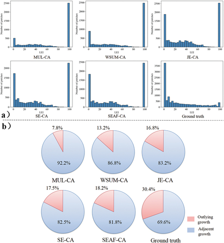
Figure 8 further shows the specific LEI distribution and the classification results of new urban patches. As shown in Figure 8(a), MUL-CA and WSUM-CA generated far fewer patches compared to the other three models, with a LEI value approaching 0. However, all models produced a greater number of patches with a LEI value approaching 100 compared to the actual observations. This discrepancy can be attributed to the fact that models usually predict non-urban areas surrounded by urban areas to have high development potential, while in reality, the development of these areas may be restrained by policies (for example, the 14th Five-Year Plan for Territorial Space Development of Wuhan prohibits excessive development of green spaces). In Figure 8(b), the proportion of outlying growth of the proposed SEAF-CA was the closest to reality, achieving 18.2%, while that of the most typical model, i.e. MUL-CA, was only 7.8%. The comparison of SE-CA with JE-CA and SEAF-CA respectively demonstrates that both of the proposed modules can increase the proportion of simulated outlying growth.

Figure 8. Simulation results of different models; (a) LEI distribution of new urban patches; (b) Classification results of new urban patches.

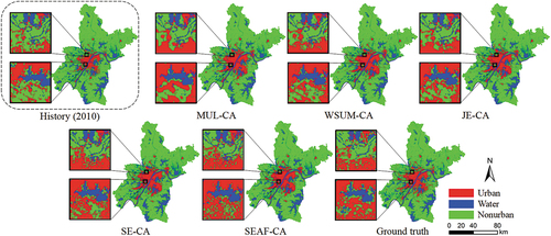
From the qualitative perspective, the difference between these simulation results and the actual urban map of Wuhan city is more intuitively displayed in Figure 9. Two small parts of the study area are selected for further visual comparison. The simulation result of SEAF-CA is visually the most consistent with the actual urban pattern: the generated patches exhibit a discrete distribution rather than only occurring in areas adjacent to existing urban areas. The simulation results for MUL-CA and WSUM-CA present a relatively compact pattern compared to the actual urban map, where the generated urban patches are more closely clustered together, reflecting obvious adjacent growth. Furthermore, although JE-CA and SE-CA perform better, there are still several mismatched predictions, mainly gathered in the bottom rectangle of Figure 9.

Figure 9. Detail of simulation results with different models.

4.3. Module function analysis

4.3.1. Effect of separate extraction module

To further study the effect of the proposed separate extraction module, attention distribution and input factor importance are successively analyzed. The former highlights the local focus of JE-CA and SE-CA on neighbor cells, while the latter provides a global comparison on the contributions made by neighboring cell states to the two models (i.e. a smaller contribution means a higher proportion of outlying growth in the simulation).

a) Attention distribution

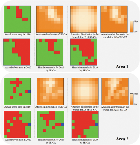
Spatial attention essentially reflects which locations are most informative for the model (Woo et al. 2018), and can characterize unequal impacts of neighboring cells in a local range. If a neighbor cell is more important for the growth of the central cell, it will be assigned higher attention. In Figure 10, two areas in Wuhan are selected, and the attention distribution of the dual branches of SE-CA and the unique branch of JE-CA are displayed. In the attention map, the gradient color for each cell indicates the attention coefficient, varying from low to high values.

In Figure 10, by learning from historical growth patterns, the NE branch exhibits an urban-weighted attention distribution, in which urban cells and their surrounding cells are assigned higher attention coefficients. The LS branch exhibits a distance-decay attention distribution, with marginal cells receiving relatively less attention. For JE-CA, the only branch also exhibits an urban-weighed attention distribution, indicating that JE-CA focuses more on urban cell states. The excessive attention to cell states causes JE-CA to prioritize the development in areas adjacent to urban lands; as a result, the potential of the areas without surrounding urban lands may be underestimated, leading to many non-urban-to-urban transformations being missed in JE-CA’s simulation result for 2020 (as shown in Figure 10). Since SE-CA has two branches with different attention distributions, the high potential of some non-urban cells without surrounding urban cells can also be captured by the LS branch, making the simulation results more consistent with the actual urban map.

Figure 10. Detail of spatial attention distribution on the selected areas.

b) Importance of input factors

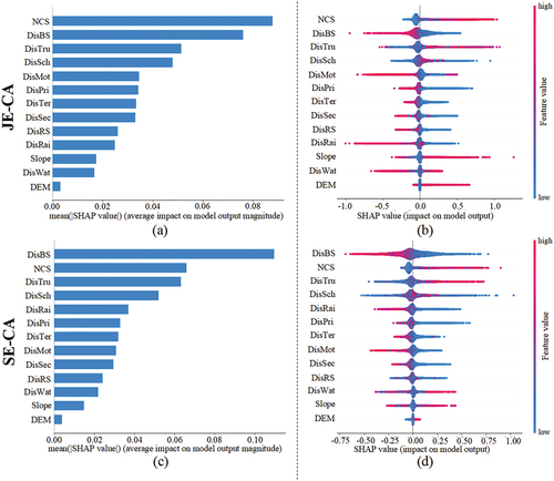
Shapley Additive explanation (SHAP) is a powerful approach for interpreting predictions of neural models, which can quantify the effects of dependent variables on independent variables based on game theory (Lundberg and Lee 2017). Here, SHAP is adopted to analyze the global importance of each input factor (Table 1) on the results obtained by SE-CA and JE-CA.

Figure 11(a,c) represents input factor importance: specifically, a larger mean absolute SHAP value indicates a greater contribution of this factor to the urban growth simulation. In Figures 11(b,d), for each factor displayed on the y-axis, each colored point represents the prediction result of one sample, and the SHAP values displayed on the x-axis denote the contribution of this factor to urban growth. The gradient color for each point indicates the average factor values of all cells in the neighborhood, varying from low (blue) to high (red) values.

In Figure 11(a), the factor “Neighboring Cell States” (NCS) is identified as the most important in JE-CA. Figure 11(b) further shows that a high NCS value (the state values of non-urban, water, and urban cells are set to 0, 1, and 2) will promote the urban growth, which indicates that the proportion of urban cells is still critical for the decisions of JE-CA. For SE-CA, the Distance to Bus Stops (DisBS) ranks first among all factors; this can be attributed to Wuhan’s adherence to the concept of “Public Transport Leading Urban Development” (Lu and Gan 2022; Yan et al. 2022). By comparison, it is obvious that JE-CA is more dependent on NCS than SE-CA, meaning that it produces a greater proportion of adjacent growth. Furthermore, the effects of DEM in both models are slight; this can be attributed to the fact that the terrain of Wuhan is entirely flat without significant topographic relief variation (Cen, Zhang, and Shi 2008).

Figure 11. Analysis of the driving factors for urban growth; (a) Relative importance for each factor of JE-CA; (b) SHAP summary plot of JE-CA; (c) Relative importance for each factor of SE-CA; (d) SHAP summary plot of SE-CA.

4.3.2. Effect of adaptive fusion module

To further study the effect of the proposed adaptive fusion module, the spatial distribution differences in the outlying growth predicted by SE-CA and SEAF-CA is first displayed; then, the adaptive weights $w_{\mathit{LS}}$ and $w_{\mathit{NE}}$ are visualized to facilitate interpreting the difference; finally, the causes of these weights are explored according to administrative division.

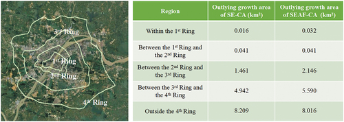
Figure 12 specifically displays the spatial distribution of the new patches belonging to the outlying growth category in the simulation results produced by SE-CA and SEAF-CA. Since ring roads play a crucial role in urban planning (Darwish, Elghazali, and Shakweer 2007), the ring roads of Wuhan are set as a basis for regional division. From Figure 12, it can be observed that within the regions surrounded by the 2^nd Ring Road, both models exhibit little outlying growth. In the regions between the 2^nd Ring Road and the 4^th Ring Road, SEAF-CA produces more outlying growth than SE-CA. Furthermore, beyond the 4^th Ring Road, although SE-CA outperforms SEAF-CA, the margin is slight at only 0.19 km².

Figure 12. Spatial distribution of the new patches belonging to the outlying growth category produced by SE-CA and SEAF-CA.

To explore why SEAF-CA obtains this spatial distribution of outlying growth, the adaptive weights $w_{\mathit{LS}}$ and $w_{\mathit{NE}}$of each cell are extracted for visualization. In Figure 13(a), each non-urban cell is assigned two distinct weights, while the white areas indicate urban and water body cells. Since the 2^nd Ring Road encircles the downtown areas of Wuhan, most of the cells within the 2^nd Ring Road are already urbanized, leading to limited development. For the regions between the 2^nd Ring Road and the 4^th Ring Road, the impact of NE is weakened by assigning low weights, while the influence of LS on urban growth is increased. Since LS and NE mainly drive outlying and adjacent growth respectively, more outlying growth occurs in these regions. Furthermore, some regions outside the 4^th Ring Road have a greater $w_{\mathit{LS}}$, while others have a greater $w_{\mathit{NE}}$; thus, SEAF-CA generates limited outlying growth beyond the 4^th Ring Road.

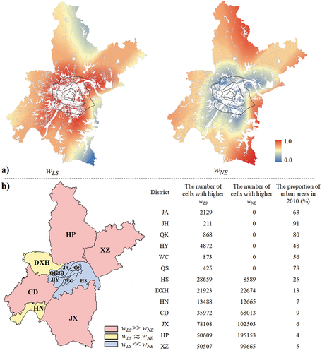
Further analysis is conducted to understand the weight distribution according to the administrative division map of Wuhan. All non-urban cells are classified into two types by comparing their respective $w_{\mathit{LS}}$ and $w_{\mathit{NE}}$. If $w_{LS}^i>w_{NE}^i$, the cell i is classified as a “cell with higher $w_{\mathit{LS}}$”; conversely, it belongs to a “cell with higher $w_{\mathit{NE}}$”. The number of two types of non-urban cells in 13 administrative districts is counted, and then these districts are divided into three categories according to the counted number, as illustrated in Figure 13(b). Furthermore, the proportion of built-up land areas for each district in 2010 is calculated, which represents the urban proportions of these districts.

In Figure 13(b), for all seven central districts of Wuhan (i.e. JA, JH, QK, HY, WC, QS, and HS), the number of non-urban cells with higher $w_{\mathit{LS}}$ is far greater than that with higher $w_{\mathit{NE}}$. Moreover, Figure 13(b) shows that the urban proportions of these districts are relatively high in 2010; in contrast, most suburban districts have more non-urban cells with higher $w_{\mathit{NE}}$, and the average urban proportion of these districts is no more than 10%. Furthermore, though HN and DXH districts have a low urban proportion, the number of both types of non-urban cells is similar in both districts. Investigation reveals that DXH and HN districts are national development zones, with GDPs that ranked first and second among all districts in 2020. Policy support and convenient infrastructure means that these two districts have great development potential and do not need to rely solely on the existing urban lands to attract development. Therefore, it can be concluded that the weight distribution is correlated with the degree of urbanization and development strategy; accordingly, high weights should be assigned to LS in highly urbanized areas and development zones to facilitate better differentiation of the growth potential of each cell.

Figure 13. Analysis of the adaptive fusion module; (a) Visualization of the adaptive weights; (b) Comparison of weights of each district in Wuhan.

4.4. Sensitivity analysis of parameters

For CA-based models, the selected neighborhood size is closely related to information extraction from the input dataset and plays a pivotal role in simulation accuracy. To explore the optimal neighborhood size of the SEAF-CA model in Wuhan, verification tests were conducted on it from 5 to 25, i.e. 450 m to 2250 m in real distance. Table 3 demonstrates that the simulation accuracy of the SEAF-CA model initially increases and then decreases with the growing neighborhood size. The peak simulation accuracy is achieved when the neighborhood size is 9. This variation trend is consistent with the findings of He et al. (2018) and Wang et al. (2019). Furthermore, it can be observed that SEAF-CA achieves the minimum FoM and also obtains the lowest MEI when the neighborhood size reaches 25. The result means that though an excessively large neighborhood size may improve the proportion of simulated outlying growth, the majority of emerging urban areas are inaccurate in the simulation. Therefore, to balance simulation accuracy with the proportion of outlying growth, a neighborhood size of 9 (i.e. 810 m) is identified as the optimal hyperparameter.

Table 3. Simulation results with different neighborhood size.

Neighborhood size	OA↑	FoM↑	MEI↓
5 × 5	91.12	20.29	50.68
9 × 9	91.20	21.06	49.98
15 × 15	91.12	20.27	50.14
19 × 19	91.09	20.01	49.76
25 × 25	91.07	19.75	45.32

5. Discussion

5.1. Advantages of the SEAF-CA model

The results in Table 2 demonstrated that the proposed SEAF-CA model achieved the best performance in the urban growth simulation of Wuhan among the developed models. The improvement can be attributed to the effectiveness of the proposed separate extraction and adaptive fusion modules.

During the extraction process, SEAF-CA is designed with a dual-path structure to independently process driving factors and cell states. The spatial attention block in each path directs the network to focus on important cells. By learning from historical growth patterns, the NE branch exhibits an urban-weighted attention distribution, in which urban cells and their surrounding cells are assigned higher attention coefficients. The LS branch exhibits a distance-decay attention distribution, with marginal cells receiving relatively less attention. This multi-attention mode addresses the issue of excessive focus on neighboring cell states in JE-CA, and then improves the accuracy of SEAF-CA.

During the fusion process, MUL-CA and WSUM-CA adopted some simple mathematical operations, and would cause that the cells with fine land suitability and adjacent to existing cities would be developed priorly. Such transition rules pose disadvantages for suburban areas with adequate resources because of their relatively low $V_{\mathit{NE}}$. While JE-CA and SEAF-CA can capture the complex nonlinear relationship between LS, NE and urban growth through learning. Additionally, SEAF-CA employs adaptive weights to characterize the relative importance of LS and NE. Higher weights are assigned to LS in highly urbanized areas and development zones, which enables a better differentiation of the growth potential in each cell and ultimately facilitates increased outlying growth.

Furthermore, the majority of model parameters in the SEAF-CA can be automatically calibrated, which avoids the problem of weak generalization introduced by manual parameterization, e.g. WSUM-CA. Since both adjacent and outlying growth are ubiquitous in urban growth, the automaticity of SEAF-CA enables its broad application in simulating urban growth across diverse contexts.

5.2. Comparison with literature

Related studies are referred to further assess our proposed SEAF-CA model, and the results of these models are collected in Table 4. All models use Wuhan as the research area, and the time spans significantly overlap with our research.

Table 4. Model comparison with related studies.

Model	Time span	FoM	Reference
S-CMM-CA	2007–2016	19.01	Wang et al. (2019)
GWLR-SLEUTH	1990–2017	16.30	Liu et al. (2020)
HYN-CA	2000–2015	22.74	Zeng et al. (2023)
SEAF-CA*	2000–2020	21.06	/

As shown in Table 4, SEAF-CA outperforms S-CMM-CA and GWLR-SLEUTH in terms of accuracy, potentially due to the omission of spatial heterogeneity when deriving transition rules in S-CMM-CA and GWLR-SLEUTH. The higher FoM of HYN-CA compared with SEAF-CA can be attributed to two reasons: (1) The simulation time span is five years shorter; (2) More social variables are used, e.g. population, GDP. Additionally, the employed Genetic Algorithm in HYN-CA comprises a significant number of empirical parameters, which will eventually lead to unstable simulation results.

Furthermore, there are many open-source software or models for urban growth simulation, e.g. FLUS (Liu et al. 2017), PLUS (Liang et al. 2021), and Terrset. FLUS and PLUS are essentially a type of MUL-CA, which multiplies land suitability with neighborhood effects in the transition rules. The limitation of MUL-CA in simulating outlying growth has been verified by our comparison experiments. SEAF-CA can improve this shortcoming of MUL-CA, achieving a higher precision in the simulation. With the Terrset software, Isinkaralar, Isinkaralar, and Bayraktar (2023) achieved a satisfying accuracy (Kappa >0.93) in Kastamonu, Türkiye. However, the calibration algorithms in the software require multiple parameters, which will be distinct in different research regions. In contrast, the proposed SEAF-CA model can automatically generate the transition rules, and thus enhance its robustness and generalization.

5.3. Limitations and future perspectives

Although the proposed SEAF-CA model has improved the ability of CA-based models to simulate outlying growth, there exist still some shortcomings of the present research. First, two CNN-based paths with identical components, are employed to extract spatial features from driving factors and cell states. Due to the greater complexity of driving factors compared to cell states, the same CNN structure makes the model more susceptible to overfitting on cell states. Second, adaptive weights are derived from geographic coordinates exclusively. Since the emergence of spatial heterogeneity is associated with multiple factors, only using geographic locations may diminish the accuracy of adaptive weights.

To make our proposed method more robust, there are also several potential points for further improvement:

1. Designing an innovative dual-path network with distinct branch structures for LS and NE extraction. LS should consider long-distance spatial dependencies, necessitating the introduction of a Transformer (Vaswani et al. 2017). In contrast, NE concentrates on local cell states, which enables the adoption of a shallower CNN.

2. Adopting more factors to derive adaptive weights. Socioeconomic index, air quality and climate data (Isinkaralar and Varol 2023; Isinkaralar, Isinkaralar, and Yilmaz 2023) can be included as inputs to improve the accuracy of adaptive weights and facilitate a comprehensive understanding of urban growth.

3. Exploring future urban growth processes under different Shared Socioeconomic Pathways (SSPs). Based on different SSPs, the urban growth pattern will differ due to various constraints. The simulations with different SSPs will make the proposed model more convincing.

6. Conclusions

In this paper, a novel CA model with separate extraction and adaptive fusion of land suitability and neighborhood effects, namely SEAF-CA, is proposed to enhance the modeling capability of outlying growth and consequently improve the simulation accuracy. An urban growth simulation of Wuhan from 2000 to 2020 is conducted to evaluate the model. Compared to three existing models (MUL-CA, WSUM-CA, and JE-CA), the proposed model achieves not only the closest outlying growth proportion to reality with an average reduction in MEI of 8.7, but also the highest simulation accuracy with an average increase in FoM of 1.1%. Our research will not only contribute to an improved understanding of the urban growth process, but also provide valuable guidance on optimizing land resources and minimizing environmental degradation, ultimately facilitating the achievement of global sustainable development goals.

Disclosure statement

No potential conflict of interest was reported by the author(s).

Additional information

Funding

This work is supported by the National Natural Science Foundation of China [Grant No. 41971348] and Hubei Luojia Laboratory [Grant No. 220100010].

Notes on contributors

Qingyang Xu

Qingyang Xu is currently pursuing the PhD degree in the State Key Laboratory of Information Engineering in Surveying, Mapping and Remote Sensing, Wuhan University, Wuhan, China. His research interests include geographic simulation and three-dimensional visualization.

Xuefeng Guan

Xuefeng Guan is currently a Professor of the State Key Laboratory of Information Engineering in Surveying, Mapping and Remote Sensing, Wuhan University, Wuhan, China. His research interests include distributed spatio-temporal databases, high-performance geospatial computing, and big spatio-temporal data mining.

Changlan Yang

Changlan Yang is currently pursuing the PhD degree in the School of Resource and Environmental Sciences at Wuhan University, China. In 2022, she received the master degree in State Key Laboratory of Information Engineering in Surveying, Mapping and Remote Sensing. Her research interest includes spatial statistic, interpretable machine learning, as well as cellular automata-based urban land use/cover change modeling.

Weiran Xing

Weiran Xing received the PhD degree from the State Key Laboratory of Information Engineering in Surveying, Mapping and Remote Sensing, Wuhan University, Wuhan, China, in 2023. His research interests include geographic simulation and computation.

Xiaoyu Chen

Xiaoyu Chen received the Bachelor’s degree in the School of Geodesy and Geomatic, Wuhan University, in 2022. Her research interests include geographic simulation and computation.

Huayi Wu

Huayi Wu is currently a Professor of the State Key Laboratory of Information Engineering in Surveying, Mapping and Remote Sensing, Wuhan University, Wuhan, China. His research interests include high-performance geospatial computing, big spatio-temporal data mining and intelligent geospatial web services.

References

- Batty, M. 1998. “Urban Evolution on the Desktop: Simulation with the Use of Extended Cellular Automata.” Environment and Planning A 30 (11): 1943–1967. https://doi.org/10.1068/a301943.
- Cao, M., S. J. Bennett, Q. Shen, and R. Xu. 2016. “A Bat-Inspired Approach to Define Transition Rules for a Cellular Automaton Model Used to Simulate Urban Expansion.” International Journal of Geographical Information Science 30 (10): 1961–1979. https://doi.org/10.1080/13658816.2016.1151521.
- Cen, Y., P. Zhang, and L. Shi. 2008. “Spatial-Temporal Characteristics of LUCC in Wuhan Area Using Satellite Data.” Paper presented at International Conference on Earth Observation Data Processing and Analysis, Wuhan, China, December. https://doi.org/10.1117/12.815940.
- Chen, G., X. Li, X. Liu, Y. Chen, X. Liang, J. Leng, X. Xu, et al. 2020. “Global Projections of Future Urban Land Expansion Under Shared Socioeconomic Pathways.” Nature Communications 11 (1). https://doi.org/10.1038/s41467-020-14386-x.
- Chen, S., Y. Feng, X. Tong, S. Liu, H. Xie, C. Gao, and Z. Lei. 2020. “Modeling ESV Losses Caused by Urban Expansion Using Cellular Automata and Geographically Weighted Regression.” Science of the Total Environment 712:136509. https://doi.org/10.1016/j.scitotenv.2020.136509.
- Clarke, K. C., and L. J. Gaydos. 1998. “Loose-Coupling a Cellular Automaton Model and GIS: Long-Term Urban Growth Prediction for San Francisco and Washington/Baltimore.” International Journal of Geographical Information Science 12 (7): 699–714. https://doi.org/10.1080/136588198241617.
- Clarke, K. C., S. Hoppen, and L. Gaydos. 1997. “A Self-Modifying Cellular Automaton Model of Historical Urbanization in the San Francisco Bay Area.” Environment and Planning B: Planning and Design 24 (2): 247–261. https://doi.org/10.1068/b240247.
- Dahal, K. R., and T. E. Chow. 2015. “Characterization of Neighborhood Sensitivity of an Irregular Cellular Automata Model of Urban Growth.” International Journal of Geographical Information Science 29 (3): 475–497. https://doi.org/10.1080/13658816.2014.987779.
- Darwish, A., S. Elghazali, and A. Shakweer. 2007. “The Effect of Ring Road Construction on Urban Land Cover Change: Greater Cairo Case Study.” Paper presented at Proceedings of the 2007 Urban Remote Sensing Joint Event, Paris, France, April. https://doi.org/10.1109/URS.2007.371763.
- Feng, Y., Y. Liu, X. Tong, M. Liu, and S. Deng. 2011. “Modeling Dynamic Urban Growth Using Cellular Automata and Particle Swarm Optimization Rules.” Landscape and Urban Planning 102 (3): 188–196. https://doi.org/10.1016/j.landurbplan.2011.04.004.
- Feng, Y., and X. Tong. 2020. “A New Cellular Automata Framework of Urban Growth Modeling by Incorporating Statistical and Heuristic Methods.” International Journal of Geographical Information Science 34 (1): 74–97. https://doi.org/10.1080/13658816.2019.1648813.
- Feng, Y., R. Wang, X. Tong, and H. Shafizadeh-Moghadam. 2019. “How Much Can Temporally Stationary Factors Explain Cellular Automata-Based Simulations of Past and Future Urban Growth?” Computers, Environment and Urban Systems 76:150–162. https://doi.org/10.1016/j.compenvurbsys.2019.04.010.
- Feng, Y., P. Wu, X. Tong, P. Li, R. Wang, Y. Zhou, J. Wang, and J. Zhao. 2022. “The Effects of Factor Generalization Scales on the Reproduction of Dynamic Urban Growth.” Geo-Spatial Information Science 25 (3): 457–475. https://doi.org/10.1080/10095020.2022.2025748.
- Fonstad, M. A. 2006. “Cellular Automata as Analysis and Synthesis Engines at the Geomorphology–Ecology Interface.” Geomorphology 77 (3–4): 217–234. https://doi.org/10.1016/j.geomorph.2006.01.006.
- Gao, C., Y. Feng, X. Tong, Z. Lei, S. Chen, and S. Zhai. 2020. “Modeling Urban Growth Using Spatially Heterogeneous Cellular Automata Models: Comparison of Spatial Lag, Spatial Error and GWR.” Computers, Environment and Urban Systems 81:101459. https://doi.org/10.1016/j.compenvurbsys.2020.101459.
- Guan, X., W. Xing, J. Li, and H. Wu. 2023. “HGAT-VCA: Integrating High-Order Graph Attention Network with Vector Cellular Automata for Urban Growth Simulation.” Computers, Environment and Urban Systems 99. https://doi.org/10.1016/j.compenvurbsys.2022.101900.
- He, J., X. Li, Y. Yao, Y. Hong, and Z. Jinbao. 2018. “Mining Transition Rules of Cellular Automata for Simulating Urban Expansion by Using the Deep Learning Techniques.” International Journal of Geographical Information Science 32 (10): 2076–2097. https://doi.org/10.1080/13658816.2018.1480783.
- Hu, Z., J. Peng, Y. Hou, and J. Shan. 2017. “Evaluation of Recently Released Open Global Digital Elevation Models of Hubei, China.” Remote Sensing 9 (3): 262. https://doi.org/10.3390/rs9030262.
- Isinkaralar, O., K. Isinkaralar, and E. P. Bayraktar. 2023. Monitoring the Spatial Distribution Pattern According to Urban Land Use and Health Risk Assessment on Potential Toxic Metal Contamination via Street Dust in Ankara, Türkiye. Environmental Monitoring and Assessment 195 (9). https://doi.org/10.1007/s10661-023-11705-9.
- Isinkaralar, O., K. Isinkaralar, and D. Yilmaz. 2023. “Climate-Related Spatial Reduction Risk of Agricultural Lands on the Mediterranean Coast in Türkiye and Scenario-Based Modelling of Urban Growth.” Environment Development and Sustainability 25 (11): 13199–13217. https://doi.org/10.1007/s10668-023-03774-0.
- Isinkaralar, O., and C. Varol. 2023. “A Cellular Automata-Based Approach for Spatio-Temporal Modeling of the City Center As a Complex System: The Case of Kastamonu, Türkiye.” Cities 132:104073. https://doi.org/10.1016/j.cities.2022.104073.
- Kamusoko, C., and J. Gamba. 2015. “Simulating Urban Growth Using a Random Forest-Cellular Automata (RF-CA) Model.” ISPRS International Journal of Geo-Information 4 (2): 447–470. https://doi.org/10.3390/ijgi4020447.
- Kasraian, D., K. Maat, and B. V. Wee. 2019. “The Impact of Urban Proximity, Transport Accessibility and Policy on Urban Growth: A Longitudinal Analysis Over Five Decades.” Environment and Planning B: Urban Analytics and City Science 46 (6): 1000–1017. https://doi.org/10.1177/2399808317740355.
- Kelobonye, K., J. C. Xia, M. S. H. Swapan, G. McCarney, and H. Zhou. 2019. “Drivers of Change in Urban Growth Patterns: A Transport Perspective from Perth, Western Australia.” Urban Science 3 (2): 40. https://doi.org/10.3390/urbansci3020040.
- Li, Q., Y. Feng, X. Tong, Y. Zhou, P. Wu, H. Xie, Y. Jin, et al. 2022. “Firefly Algorithm-Based Cellular Automata for Reproducing Urban Growth and Predicting Future Scenarios.” Sustainable Cities and Society 76:103444. https://doi.org/10.1016/j.scs.2021.103444.
- Li, X., Q. Yang, and X. Liu. 2007. “Genetic Algorithms for Determining the Parameters of Cellular Automata in Urban Simulation.” Science in China Series D: Earth Sciences 50 (12): 1857–1866. https://doi.org/10.1007/s11430-007-0127-4.
- Li, X., and A. G. O. Yeh. 2000. “Modelling Sustainable Urban Development by the Integration of Constrained Cellular Automata and GIS.” International Journal of Geographical Information Science 14 (2): 131–152. https://doi.org/10.1080/136588100240886.
- Liang, X., Q. Guan, K. C. Clarke, S. Liu, B. Wang, and Y. Yao. 2021. “Understanding the Drivers of Sustainable Land Expansion Using a Patch-Generating Land Use Simulation (PLUS) Model: A Case Study in Wuhan, China.” Computers, Environment and Urban Systems 85:101569. https://doi.org/10.1016/j.compenvurbsys.2020.101569.
- Liu, D., K. C. Clarke, and N. Chen. 2020. “Integrating Spatial Nonstationarity into SLEUTH for Urban Growth Modeling: A Case Study in the Wuhan Metropolitan Area.” Computers, Environment and Urban Systems 84:101545. https://doi.org/10.1016/j.compenvurbsys.2020.101545.
- Liu, X., X. Li, Y. Chen, Z. Tan, S. Li, and B. Ai. 2010. “A New Landscape Index for Quantifying Urban Expansion Using Multi-Temporal Remotely Sensed Data.” Landscape Ecology 25 (5): 671–682. https://doi.org/10.1007/s10980-010-9454-5.
- Liu, X., X. Li, L. Liu, J. He, and B. Ai. 2008. “A Bottom-Up Approach to Discover Transition Rules of Cellular Automata Using Ant Intelligence.” International Journal of Geographical Information Science 22 (11–12): 1247–1269. https://doi.org/10.1080/13658810701757510.
- Liu, X., X. Liang, X. Li, X. Xu, J. Ou, Y. Chen, S. Li, S. Wang, and F. Pei. 2017. “A Future Land Use Simulation Model (FLUS) for Simulating Multiple Land Use Scenarios by Coupling Human and Natural Effects.” Landscape and Urban Planning 168:94–116. https://doi.org/10.1016/j.landurbplan.2017.09.019.
- Liu, X., L. Ma, X. Li, B. Ai, S. Li, and Z. He. 2014. “Simulating Urban Growth by Integrating Landscape Expansion Index (LEI) and Cellular Automata.” International Journal of Geographical Information Science 28 (1): 148–163. https://doi.org/10.1080/13658816.2013.831097.
- Liu, Y., Q. He, R. Tan, Y. Liu, and C. Yin. 2016. “Modeling Different Urban Growth Patterns Based on the Evolution of Urban Form: A Case Study from Huangpi, Central China.” Applied Geography 66:109–118. https://doi.org/10.1016/j.apgeog.2015.11.012.
- Lu, H., and H. Gan. 2022. “Evaluation and Prevention and Control Measures of Urban Public Transport Exposure Risk Under the Influence of COVID-19—Taking Wuhan As an Example.” PLOS ONE 17 (6): e0267878. https://doi.org/10.1371/journal.pone.0267878.
- Lundberg, S. M., and S. I. Lee. 2017. “A unified approach to interpreting model predictions.” Paper presented at Proceedings of the Advances in Neural Information Processing Systems, Long Beach, USA, December 4-9.
- Masoumi, Z., and J. V. Genderen. 2023. “Artificial Intelligence for Sustainable Development of Smart Cities and Urban Land-Use Management.” Geo-Spatial Information Science 1–25. https://doi.org/10.1080/10095020.2023.2184729.
- Meng, Y., M. S. Wong, M. P. Kwan, J. Pearce, and Z. Feng. 2023. “Assessing Multi-Spatial Driving Factors of Urban Land Use Transformation in Megacities: A Case Study of Guangdong–Hong Kong–Macao Greater Bay Area from 2000 to 2018.” Geo-Spatial Information Science 1–17. https://doi.org/10.1080/10095020.2023.2255033.
- Moghadam, H. S., and M. Helbich. 2013. “Spatiotemporal Urbanization Processes in the Megacity of Mumbai, India: A Markov Chains-Cellular Automata Urban Growth Model.” Applied Geography 40:140–149. https://doi.org/10.1016/j.apgeog.2013.01.009.
- Mustafa, A., A. Heppenstall, H. Omrani, I. Saadi, M. Cools, and J. Teller. 2018. “Modelling Built-Up Expansion and Densification with Multinomial Logistic Regression, Cellular Automata and Genetic Algorithm.” Computers, Environment and Urban Systems 67:147–156. https://doi.org/10.1016/j.compenvurbsys.2017.09.009.
- Pal, S., and S. K. Ghosh. 2017. “Rule Based End-To-End Learning Framework for Urban Growth Prediction.” arXiv preprint arXiv:1711.10801.
- Qian, Y., W. Xing, X. Guan, T. Yang, and H. Wu. 2020. “Coupling Cellular Automata with Area Partitioning and Spatiotemporal Convolution for Dynamic Land Use Change Simulation.” Science of the Total Environment 722. https://doi.org/10.1016/j.scitotenv.2020.137738.
- Southworth, M., and P. M. Owens. 1993. “The Evolving Metropolis: Studies of Community, Neighborhood, and Street Form at the Urban Edge.” Journal of the American Planning Association 59 (3): 271–287. https://doi.org/10.1080/01944369308975880.
- Vaswani, A., N. Shazeer, N. Parmar, J. Uszkoreit, L. Jones, A. N. Gomez, L. Kaiser, and I. Polosukhin. 2017. “Attention Is All You Need.” Paper presented at Proceedings of the Advances in Neural Information Processing Systems, Long Beach, USA, December 4-9.
- Wang, J., M. Hadjikakou, R. J. Hewitt, and B. A. Bryan. 2022. “Simulating Large-Scale Urban Land-Use Patterns and Dynamics Using the U-Net Deep Learning Architecture.” Computers, Environment and Urban Systems 97:101855. https://doi.org/10.1016/j.compenvurbsys.2022.101855.
- Wang, W., L. Jiao, T. Dong, Z. Xu, and G. Xu. 2019. “Simulating Urban Dynamics by Coupling Top-Down and Bottom-Up Strategies.” International Journal of Geographical Information Science 33 (11): 2259–2283. https://doi.org/10.1080/13658816.2019.1647540.
- White, R., and G. Engelen. 1993. “Cellular Automata and Fractal Urban Form: A Cellular Modelling Approach to the Evolution of Urban Land-Use Patterns.” Environment and Planning A 25 (8): 1175–1199. https://doi.org/10.1068/a251175.
- Woo, S., J. Park, J. Y. Lee, and I. S. Kweon. 2018. “Cbam: Convolutional Block Attention Module.” Paper presented at Proceedings of the European Conference on Computer Vision, Munich, Germany, September 8-14.
- Wu, F. 2002. “Calibration of Stochastic Cellular Automata: The Application to Rural-Urban Land Conversions.” International Journal of Geographical Information Science 16 (8): 795–818. https://doi.org/10.1080/13658810210157769.
- Wu, H., L. Zhou, X. Chi, Y. Li, and Y. Sun. 2012. “Quantifying and Analyzing Neighborhood Configuration Characteristics to Cellular Automata for Land Use Simulation Considering Data Source Error.” Earth Science Informatics 5 (2): 77–86. https://doi.org/10.1007/s12145-012-0097-8.
- Xing, W., Y. Qian, X. Guan, T. Yang, and H. Wu. 2020. “A Novel Cellular Automata Model Integrated with Deep Learning for Dynamic Spatio-Temporal Land Use Change Simulation.” Computers & Geosciences 137:104430. https://doi.org/10.1016/j.cageo.2020.104430.
- Xu, X., D. Zhang, X. Liu, J. Ou, and X. Wu. 2022. “Simulating Multiple Urban Land Use Changes by Integrating Transportation Accessibility and a Vector-Based Cellular Automata: A Case Study on City of Toronto.” Geo-Spatial Information Science 25 (3): 439–456. https://doi.org/10.1080/10095020.2022.2043730.
- Yamashita, R., M. Nishio, R. K. G. Do, and K. Togashi. 2018. “Convolutional Neural Networks: An Overview and Application in Radiology.” Insights into Imaging 9 (4): 611–629. https://doi.org/10.1007/s13244-018-0639-9.
- Yan, X., Y. Feng, X. Tong, P. Li, Y. Zhou, P. Wu, H. Xie, et al. 2021. “Reducing Spatial Autocorrelation in the Dynamic Simulation of Urban Growth Using Eigenvector Spatial Filtering.” International Journal of Applied Earth Observation and Geoinformation 102:102434. https://doi.org/10.1016/j.jag.2021.102434.
- Yan, X., J. Zhou, F. Sheng, and Q. Niu. 2022. “Influences of Built Environment at Residential and Work Locations on Commuting Distance: Evidence from Wuhan, China.” ISPRS International Journal of Geo-Information 11 (2): 124. https://doi.org/10.3390/ijgi11020124.
- Yang, J., and X. Huang. 2021. “The 30 M Annual Land Cover Dataset and Its Dynamics in China from 1990 to 2019.” Earth System Science Data 13 (8): 3907–3925. https://doi.org/10.5194/essd-13-3907-2021.
- Yang, Q., X. Li, and X. Shi. 2008. “Cellular Automata for Simulating Land Use Changes Based on Support Vector Machines.” Computers & geosciences 34 (6): 592–602. https://doi.org/10.1016/j.cageo.2007.08.003.
- Zeng, H., H. Wang, B. Zhang, and Q. Wang. 2023. “A Methodology to Quantify the Neighborhood Decay Effect of Urban Cellular Automata Models.” International Journal of Geographical Information Science 37 (6): 1236–1263. https://doi.org/10.1080/13658816.2023.2186412.
- Zhai, Y., Y. Yao, Q. Guan, X. Liang, X. Li, Y. Pan, H. Yue, Z. Yuan, and J. Zhou. 2020. “Simulating Urban Land Use Change by Integrating a Convolutional Neural Network with Vector-Based Cellular Automata.” International Journal of Geographical Information Science 34 (7): 1475–1499. https://doi.org/10.1080/13658816.2020.1711915.
- Zhang, B., S. Hu, H. Wang, and H. Zeng. 2023. “A Size-Adaptive Strategy to Characterize Spatially Heterogeneous Neighborhood Effects in Cellular Automata Simulation of Urban Growth.” Landscape and Urban Planning 229. https://doi.org/10.1016/j.landurbplan.2022.104604.
- Zhang, B., and C. Xia. 2022. “The Effects of Sample Size and Sample Prevalence on Cellular Automata Simulation of Urban Growth.” International Journal of Geographical Information Science 36 (1): 158–187. https://doi.org/10.1080/13658816.2021.1931237.
- Zhao, D., and T. F. Sing. 2017. “Air Pollution, Economic Spillovers, and Urban Growth in China.” The Annals of Regional Science 58 (2): 321–340. https://doi.org/10.1007/s00168-016-0783-4.
- Zhu, Q., M. Zeng, P. Jia, M. Guo, X. Liang, and Q. Guan. 2023. “Measuring the Urban Sprawl Based on Economic-Dominated Perspective: The Case of 31 Municipalities and Provincial Capitals.” Geo-Spatial Information Science 1–18. https://doi.org/10.1080/10095020.2023.2202201.