Adaptive Multiple Comparison Sequential Design (AMCSD) for clinical trials

ABSTRACT

We propose an adaptive sequential testing procedure for clinical trials that test the efficacy of multiple treatment options, such as dose/regimen, different drugs, sub-populations, endpoints, or a mixture of them in one trial. At any interim analyses, sample size re-estimation can be conducted, and any option can be dropped for lack of efficacy or unsatisfactory safety profile. Inference after the trial, including p-value, conservative point estimate and confidence intervals, are provided.

KEYWORDS:

• Brownian motion approximation
• multiple comparison
• adaptive sequential design
• sample size re-estimation
• treatment selection

1. Introduction

Clinical trials are expensive. Moore et al. (2018) analyzed the costs for the pivotal trials for novel therapeutic agents approved by the US Food and Drug Administration during the period of 2015–2016: “Trials designed with placebo or active drug comparators had an estimated mean cost of $35.1 million (95% CI, $25.4 million-$44.8 million)”. The cost for the most expansive trial in this report was $346.8 million. Many efforts have been made to reduce the cost. One category of such efforts is the multi-arm-multi-stage (MAMS) design. Such a design essentially combines several trials into one, and multiple treatments are compared to a shared single control arm, hence eliminating the need for several control arms in separate trials and reduces the total sample size.

The main advantage of MAMS is cost efficiency (Freidlin et al. 2008 ; Jaki and Hampson 2016; Jaki and Wason 2018) from this sample size reduction. Other benefits of reduced sample size include the shortening of trial duration and the reduction of burden of patient recruitment, especially in trials that require a large number of patients per treatment arm, or in rare diseases where the enrollment is extremely difficult due to small patient population. For example, the European Medicines Agency issued a “Call to pool research resources into large multi-centre, multi-arm clinical trials to generate sound evidence on COVID-19 treatments” (19 March 2020). The MAMS design has been adopted in practice, e.g., i) The multi-arm optimization of stroke thrombosis (National Institute of Health n.d.); ii) A 3-arm multi-center, randomized controlled study comparing transforaminal corticosteroid, transforaminal etanercept and transforaminal saline for lumbosacral radiculopathy (clinicaltrials.gov, NCT00733096).

The main statistical challenges in such trials include: i) Family-wise error (FWE) control with simultaneous testing of multiple hypotheses at multiple time points. An optimal control is such that the FWE never exceeds the nominal error level but can be equal to the nominal level under certain conditions. A conservative control is such that the FWE never reaches the nominal level under any situation. The Bonferroni method is an example of conservative control. Conservative control will lead to reduced power. Hence, methods that achieve less conservative or optimal control are more preferable; ii) Sample size and power calculation (as always, such calculations involve assumptions on the effect size) which are important to trial planning; iii) The assumptions for sample size calculation could be inaccurate (due to uncertainty about effect sizes) and adaptive measures, such as sample size re-estimation (SSR), may be desirable to achieve adequate power. To obtain a proper new sample size, a method for calculating conditional power will be necessary. Further, FWE must be adequately controlled when adaptations are applied to the trial; iv) Inference must be made after the completion of the trial. Hence, p-values, estimates of the effect sizes, confidence intervals are desirable. v) When adaptations are made to the trial, inferences will be more complicated, but their relevance and importance is not reduced; vi) Computations with multiple tests at multiple time points could be complicated and very time consuming. A MAMS procedure won’t be practical without efficient means of computations (e.g., Ghosh et al. 2017).

In addition to the need for investigating multiple treatments in one trial as in MAMS, there are also other types of trials that share the same statistical challenges as MAMS. These include trials that investigate multiple sub-populations (FDA guidance [population enrichment], 2019), and/or multiple endpoints (FDA guidance [adaptive design], 2019), in one trial. Statistical solutions for MAMS can also be applied to such trials. Sequential designs and adaptive sequential designs that include multiple options such as multiple treatment (e.g., doses/regimens), multiple sub- populations (FDA guidance [population enrichment], 2019), and/or multiple endpoints (FDA guidance [adaptive design], 2019), may be more generally named as (adaptive) multiple comparison sequential designs (AMCSD/MCSD). In this article, we propose such a procedure that addresses all of the above-mentioned statistical issues.

2. Background and features of proposed method

2.1. Background

Take a trial that tests multiple doses as an example for MAMS, other situations can be dealt with similarly. Suppose that the trial includes $\mathit{M}$ dose groups and a control arm, and a total of $\mathit{K}$ interim/final analyses. Let ${\theta }_m$ (m = 1,…, M) be the efficacy for each dose being considered, larger $\mathit{\theta }$ indicates better efficacy. Let $\vec{\theta }=\left({\theta }_1,\dots ,{\theta }_M\right)$. Let the related hypotheses for each dose comparison be: null hypothesis $H_{0,\mathit{m}}$: ${\theta }_m=0$, and one-sided alternative hypothesis $H_{\mathit{a},\mathit{m}}$: ${\theta }_m>0$. The overall null hypothesis is $H_0=H_0^M={\cap }_{m=1}^M{H}_{0,\mathit{m}}$: $\vec{\theta }=\vec{0}$. Or equivalently, ${\theta }_{\mathit{max}}=\mathit{max}\left({\theta }_1,\dots ,{\theta }_M\right)=0$. The overall alternative hypothesis is $H_a={\left(H_0\right)}^{\mathit{c}}={\cup }_{m=1}^M{H}_{\mathit{a},\mathit{m}}$, at least one ${\theta }_m>0$, or equivalently, ${\theta }_{\mathit{max}}>0$. At the $\mathit{i}$-th interim analysis, each of the $\mathit{M}$ parameters ${\theta }_1,\dots ,{\theta }_M$, is associated with an estimate ${\hat{\theta }}_{\mathit{i},\mathit{m}}$, and the standard error $\mathit{s}.\mathit{e}.({\hat{\theta }}_{\mathit{i},\mathit{m}}\mathit{\hspace{0.17em}})$, $\mathit{m}=1,\dots ,\mathit{M}$. The comparison of each dose and the control is associated with a Wald statistic $Z_{\mathit{i},\mathit{m}}={\hat{\theta }}_{\mathit{i},\mathit{m}}/\mathit{s}.\mathit{e}.({\hat{\theta }}_{\mathit{i},\mathit{m}}\mathit{\hspace{0.17em}})$, or equivalently, a score function $S_{\mathit{i},\mathit{m}}={\hat{\theta }}_{\mathit{i},\mathit{m}}/[\mathit{s}.\mathit{e}.({\hat{\theta }}_{\mathit{i},\mathit{m}}\mathit{\hspace{0.17em}}){]}^2$. At each interim analysis, these Wald statistics or score functions form an $\mathit{M}$ -dimensional random vector, with a multi-variate normal distribution. Hence, there will be a total of $\mathit{M}\times \mathit{K}$ Wald statistics or score functions. Thus a MAMS trial involves the testing of these $\mathit{M}\times \mathit{K}$ test statistics and the conditional probabilities associated with the adaptive decisions during the trial. A fundamental challenge is to control family-wise error (FWE). A major distinction between the Wald statistics and the score functions is that the score function has independent increment and is approximately a Brownian motion (Jennison and Turnbull 1997). The score function vectors form a multi-dimensional Markov process with independent increment. The research into the MAMS design can be traced at least back to 1989 (Bauer et al. 2015). Several methods employ Dunnett’s multiple-testing procedure (on each $\mathit{M}$ -dimensional random vector of the Wald statistics) in some form (Magirr et al. 2012; Wason et al. 2016, 2017). Stallard and Friede (2008) uses the score function and Dunnett’s procedure (on each $\mathit{M}$ -dimensional random vector of the score functions) to construct a group-sequential design where a set number of treatment options are dropped at each interim analysis. The null hypothesis is rejected if the test statistic is above a predefined efficacy threshold. It requires the number of doses to be dropped at any given interim analysis to be pre-specified, hence limiting its flexibility. Bretz et al. (2006) used closed testing procedures and combination tests to control the type-I error whilst allowing many modifications to be made at the interim. The control of FWE in these methods is a two-level procedure, one level controls the FWE for each $\mathit{M}$ -dimensional random vector at each interim analysis, then the combined FWE at all interim/final analyses is controlled. A drop-the-loser approach proposed by Chen et al. (2010) utilizes the multi-variate normality of the Wald statistics and constructed a sequential design with interim analyses that is parallel to the usual group sequential design for comparing one experimental treatment and a control (e.g., O’Brien and Fleming 1979; Pocock 1977). It requires the assumption that the covariance coefficient to be ½, this limits the types of trials the method can be applied to. This method does not use multi-testing procedures, such as the Dunnett’s procedure or closed testing procedure to control the FWE. All the above-mentioned methods do not provide p-values and estimates, and there are no sample-size re-estimations. Gao et al. (2014) considers an adaptive group sequential design using a Markov process (formed by the score functions) approach. The procedure does not use the Dunnett method or closed testing procedure. Instead, it uses Markov transition probabilities for the calculations of the critical boundaries, type I error control and sample size re-estimation. It provided exact FWE control in the strong sense, sample size calculation, and sample size re-estimation. It is limited to cases in which the covariance matrix of the score functions are known (it does include cases in which the covariance coefficient is ½ such as in Stallard and Friede 2008; or; Chen et al. 2010). Gao et al. (2014) only included p-values but not parameter estimates after the trial. Both Chen et al. (2010) and Gao et al. (2014) use the correlations of the $\mathit{K}$ $\mathit{M}$- dimensional random vectors to control the FWE, instead of the two level FWE control such as those by Bauer et al. (2015),Wason et al. (2016), Wason et al. (2017), Magirr et al. (2012), Stallard and Friede (2008), Bretz et al. (2006). All of previous literature, including Chen et al. (2010) and Gao et al. (2014) investigates the properties of $\mathit{K}$ separate $\mathit{M}$- dimensional random vectors (Chen et al. 2010 uses the Wald statistics, and Gao et al. 2014 uses the score functions). The algorithm in Gao et al. (2014) uses the Markov transition probabilities which involves iterative multi-dimensional integrals and is very time-consuming (see Ghosh et al. 2017). Ghosh et al. (2017) proposed new computing algorithm which linearized the multi-dimensional integrals and greatly reduced the time for the computations, but the computing code is very complicated.

2.2. Features of proposed method

In the theory of GSD that compares a test treatment and a control, the recursive algorithm of Armitage et al. (1969), which involves iterative integrals, has been essential for the derivation of critical boundary, sample size/power calculation (e.g., Jennison and Turnbull 2000). In a GSD, a score function $\mathit{S}\left(\mathit{\hspace{0.17em}}\mathit{t}\right)$ (is the information time) can be created, which is approximately a Brownian motion (Jennison and Turnbull 1997) and also a one-dimensional Markov process. All the methodologies regarding the GSD can be explained using intuitions about the trajectories of the score function as a Brownian motion/Markov process (e.g., Gao et al. 2008, 2013). With this intuition, a Brownian trajectory corresponds to the score function curve of an infinitely long clinical trial. A GSD involves $\mathit{K}$ information time points $0<t_1<\dots <t_K$, score function values $\mathit{S}\left(\mathit{\hspace{0.17em}}{t}_1\right),\dots ,\mathit{S}\left(\mathit{\hspace{0.17em}}{t}_K\right)$ can be obtained, which has a joint multivariate normal distribution, with a $\mathit{K}\times \mathit{K}\mathit{\hspace{0.17em}}$covariance matrix. The entire theory of GSD can be described using this multivariate normal distribution and some calculus (see online supporting material, section 1), without using the recursive algorithm. We refer to this as the Brownian motion approximation (BMA) approach for GSD. In this article, we use a parallel BMA approach on MCSD/AMCSD and improve upon Gao et al. (2014). For the comparison of the $\mathit{m}$-th dose (suppose that there are $\mathit{m}$ doses) and the control, a score function $S_m\left(\mathit{t}\right)$ can be created. Suppose that there are $\mathit{K}$ interim analysis/final analyses at information time points $0<t_1<\dots <t_K$. There will be $\mathit{M}\times \mathit{K}$ score functions, $S_m\left(\mathit{\hspace{0.17em}}{t}_1\right),\dots ,S_m\left(\mathit{\hspace{0.17em}}{t}_K\right)$, $\mathit{m}=1,\dots ,\mathit{M}$. These score functions have a joint multivariate normal distribution, with an $\left(\mathit{M}\times \mathit{K}\mathit{\hspace{0.17em}}\right)\times \left(\mathit{M}\times \mathit{K}\mathit{\hspace{0.17em}}\right)$ dimensional covariance matrix. All previous methods on MAMS in the literature use some kind of iterative algorithm (e.g., see citations of literature in previous section). By using the multivariate normal distribution of these $\mathit{M}\times \mathit{K}$ score functions, our proposed method does not use any iterative algorithm, and is thus different from all methods in the literature. The proposed procedure is entirely parallel to that of the BMA approach for GSD/ASD (see online supporting material, section 1): i) Similar sample size and power calculations (i.e., using integration over multivariate normal distribution); ii) similar type I error control using critical boundaries(i.e., using integration over multivariate normal distribution); iii) Similar SSR using conditional power; iv) Similar type I error/FWE control when there is sample size change (i.e. maintaining conditional type I error/FWE, as in Gao et al. 2008; The conditional type I error/FWE are obtained by using integration over multivariate normal distribution); v) Similar logic for calculating inferences (i.e., using the inverse of a monotone function to obtain point estimate, p-value, and confidence interval, as in Gao et al. 2013); vi) Similar logic (using backward image, Gao et al. 2013) for obtaining inferences when there was sample size change.

With (and because of) this algorithm, the proposed procedure possesses the following features: i) FWE control is optimal. The FWE equals to the nominal error level in the special case when the off-diagonal elements of the covariance matrix are known (e.g., off diagonal elements are 0.5, or zero) and the “play the winner” rule (i.e., selecting the best observed treatment option) is applied for adaptation and for hypothesis testing. The FWE is less than the nominal level (i.e., conservative) in all other situations. ii) Sample size and power calculation are exact for the special case and conservative in other situations; iii) Sample size re-estimation is precise in the special case when the observed efficacy equals the true efficacy. Conditional FWE is controlled exactly in the special case and conservative otherwise, hence the overall FWE is controlled; iv) Conservative inferences: Exact inferences require knowledge of the configuration of the vector $\vec{\theta }=\left({\theta }_1,\dots ,{\theta }_M\right)$ and the covariance matrix. But neither is known in actual trials and exact inferences are not possible. Conservative estimates such as p-values (larger than the true value), point estimate (smaller than the true value), and confidence interval (wider than the exact interval) can be obtained with the proposed procedure to make valid conclusions about the efficacy. v) Conservative inferences with adaptation (such as SSR and dropping some comparisons (e.g., ineffective doses) can also be obtained; vi) Computation efficiency: Gao et al. (2014) used iterative multiple integration to calculate probabilities. The iterations are very time consuming (see Ghosh et al. 2017, for discussions). Because the new proposed algorithm does not use iterations, it does not require long computation time. Sample size and power calculation takes about 2–3 seconds. The algorithm is also much simpler than that of Ghosh et al. (2017). vii) By using Slepian’s lemma (Huffer 1986; Slepian 1962), the design can be applied to cases in which the covariance coefficients are not known. Hence, the design can be applied not only to dose selections, but also to trials involving different regimens, drugs, or population enrichment. Further, conservative point estimates and confidence intervals, with or without sample size change, are provided. viii) Lastly, all previous methods only test the overall null hypothesis $H_0^M={\cap }_M^{m=1}{H}_{0,\mathit{m}}$ that at least one experimental treatment is superior to the control. Our method includes a closed testing procedure (similar to an example that uses a modified Dunnett’s testing in Marcus et al. 1976) that can test all the $\mathit{l}$-level null hypotheses $H_0^l={\cap }_{m\in Q_l}{H}_{0,\mathit{m}}$ (a $Q_l$ contains $\mathit{l}$-elements) for all $1\le \mathit{l}\le \mathit{M}$, and can be used to reject multiple individual null hypotheses $H_{0,\mathit{m}}$. All $\mathit{l}$-level testing will use a common $\mathit{l}$-level critical boundaries.

We refer our method as the Brownian motion approximation (BMA) approach for MCSD, which reduces to GSD/ASD when $\mathit{M}=1$. The BMA approach does not require in-depth knowledge of either Brownian motion or Markov processes. It only uses calculus and four basic (widely known) properties of Brownian motion: i) It is additive: $\mathit{B}\left(\mathit{t}\right)+\mathit{B}\left(\mathit{u}\right)=\mathit{B}\left(\mathit{t}+\mathit{u}\right)$; ii) It has independent increment; iii) $\mathit{covB}\left(t_i\right),\mathit{B}\left(t_j\right)=\mathit{min}\left\{t_i,t_j\right\}$; iv) For $0<t_1<..<t_K$, $\left(\mathit{B}\left(t_1\right),\dots ,\mathit{B}\left(t_K\right)\right)$ has a joint multivariate normal distribution (e.g., Jennison and Turnbull 2000; Whitehead 1997). An MCSD/AMCSD design is an adaptive design. The FDA guidance on adaptive designs (2019) summarized the major potential advantages of adaptive designs: a) Statistical efficiency; b) Ethical considerations; c) Improved understanding of drug effects; d) Acceptability to stakeholders. In the same guidance, the FDA (2019) recommended that three statistical principles should be satisfied: a) Controlling the Chance of Erroneous Conclusions (type I error control); b) Estimating Treatment Effects (valid inference, including point estimate, two-sided confidence interval, and p-value); c) Trial Planning (including sample size/power calculation); (The FDA guidance (2019) also included a fourth principle, which is operational: d) Maintaining Trial Conduct and Integrity). Our method, the MCSD/AMCSD, satisfies all the three statistical principles in the FDA guidance (2019). The MCSD/AMCSD is supported by the DACT (Design and Analysis for Clinical trials) software at https://www.innovativstat.com/software.html (The software is free for academic researchers). Computation codes are available upon request.

3. Method

3.1. Score function and GSD

To demonstrate the similarities between GSD and MCSD, we first describe the GSD using BMA. In a GSD, one experimental treatment is compared with a control. Let $\mathit{\theta }$ be the parameter of interest, larger $\mathit{\theta }$ indicates better efficacy, and the null hypothesis is $H_0$: $\mathit{\theta }=0$, and the alternative hypothesis is $H_a$: $\mathit{\theta }>0$, Let $\hat{\theta }$ be an unbiased estimate, and $\mathit{s}.\mathit{e}.\left(\hat{\theta }\right)$the standard error. Then, $\mathit{Z}=\hat{\theta }/\mathit{s}.\mathit{e}.\left(\hat{\theta }\right)$ is the Wald statistics, and the score function is $\mathit{S}=\mathit{Z}/\mathit{s}.\mathit{e}.\left(\hat{\theta }\right)=\hat{\theta }/{\left(s.e.\left(\hat{\theta }\right)\right)}^2$. The Fisher’s information time is $\mathit{t}={\left(s.e.\left(\hat{\theta }\right)\right)}^{-2}$. Approximately, $\mathit{S}\approx \mathit{W}\left(\mathit{t}\right)=\mathit{B}\left(\mathit{t}\right)+\mathit{\theta t}\sim \mathit{N}\left(\mathit{\theta t},\mathit{t}\right)$ (Jennison and Turnbull 1997). The GSD (O’Brien and Fleming 1979; Pocock 1977) was based on the Wald statistics. Interim analyses are planned, to be performed at information time points $t_1<\dots <t_K=\mathit{T}$. Critical boundaries $c_1,\dots ,c_K$ are chosen such that $H_0$ is rejected in favor of $H_a$ if the event ${\cup }_K^{i=1}\left(Z_i\ge c_i\right)$ is observed ($Z_i=\mathit{Z}\left(t_i\mathit{\hspace{0.17em}}\right)$ is the Wald statistics at $t_i$). Type I error is controlled by requiring $\mathit{P}{\cup }_K^{i=1}\left(Z_i\ge c_i\right)\le \mathit{\alpha }/2$.With the BMA, the score functions are $\mathit{S}\left(t_i\right)=Z_i/\sqrt{t_i}$. Let $e_i=c_i\sqrt{t_i}$ and name the $e_i$ ‘s as the “exit” boundaries. The rules of a GSD can be equivalently stated as $\mathit{P}{\cup }_K^{i=1}\left(\mathit{S}\left(t_i\right)\ge e_i\right)\le \mathit{\alpha }/2$. The random vector $\vec{S}=\left(\mathit{S}\left(t_1\right),\dots ,\mathit{S}\left(t_K\right)\right)$ has a multivariate normal distribution, with a $\mathit{K}\times \mathit{K}\mathit{\hspace{0.17em}}$covariance matrix. All probabilities such as sample size and power calculation, type I error, can be calculated using multivariate integration on $\vec{S}$ without using the recursive algorithm (Armitage et al, 1969). A brief description is provided in the online supporting material.

3.2. The proposed MCSD

3.2.1. The vector of the score functions

Each of the $\mathit{M}$ parameters ${\theta }_1,\dots ,{\theta }_M$, is associated with an estimate ${\hat{\theta }}_{\mathit{m}}$ (at any information time $t_m$) and a score function $S_m\left({\hat{\theta }}_{\mathit{m}}\mathit{\hspace{0.17em}}\right)={\hat{\theta }}_{\mathit{m}}/{\left[s.e.\left({\hat{\theta }}_{\mathit{m}}\mathit{\hspace{0.17em}}\right)\right]}^2=S_m\left(t_m\right)\approx W_{t_m}=W_m\left(t_m\right)$$=B_m\left(t_m\right)+\mathit{\hspace{0.17em}}{\theta }_m\mathit{\hspace{0.17em}}{t}_m\sim \mathit{N}\left({\theta }_m\mathit{\hspace{0.17em}}{t}_m,\mathit{\hspace{0.17em}}{t}_m\right)$.

3.2.2. Hypothesis testing and type I error control

The trial will include a total of K analyses including the interim analyses and the final analysis. Let $t_{\mathit{m},\mathit{i}}$ be the information time for the $\mathit{m}-$th component $W_m\left(\mathit{t}\right)$ at the i-th interim analysis. For each, $t_{\mathit{m},1}<\dots <t_{\mathit{m},\mathit{K}}$. This forms an information vector at each interim analysis, ${\vec{t}}_{\mathit{i}}=\left(t_{1,\mathit{i}},\dots ,t_{\mathit{M},\mathit{i}}\right)$, i = 1, …, K. Type I error control is achieved by selecting critical boundaries $c_1$, …, $c_K$ such that the null hypothesis $H_0=H_0^{\left(M\right)}=\cap \mathit{\hspace{0.17em}}\mathit{m}=1\mathit{M}{H}_{0,\mathit{m}}$ is rejected if $\cup \mathit{\hspace{0.17em}}\mathit{i}=1\mathit{K}\cup \mathit{\hspace{0.17em}}\mathit{m}=1\mathit{M}\left(W_m\left(t_{\mathit{m},\mathit{i}}\right)\ge c_i\sqrt{t_{\mathit{m},\mathit{i}}}\right)$ is observed. The type I error is controlled if $c_1$, …, $c_K$ satisfy the condition that $\mathit{P}\cup \mathit{i}=1\mathit{K}\cup \mathit{m}=1\mathit{M}\left(W_m\left(t_{\mathit{m},\mathit{i}}\right)\ge c_i\sqrt{t_{\mathit{m},\mathit{i}}}\right)\vec{\theta }=\left(0,\dots ,0\right)\le \mathit{\alpha }/2$.

3.2.3. The closed testing procedure

3.2.3.1. The L-level tests and critical boundaries

The closed testing procedure has been used to control FWE for testing $H_0^{\left(M\right)}$ (e.g., Bretz et al. 2006). We propose the use of the closed testing procedure for a different purpose. Marcus et al. (1976) included an example for closed testing procedure by modifying Dunnett (1955) in which multiple individual null hypotheses can be rejected using different levels of rejection criteria. Such a procedure is more powerful than a single criterion that only tests $H_0^{\left(M\right)}$. The proposed closed testing procedure is similar to this example. With this closed testing procedure, our proposed design is more powerful than the methods in the literature (e.g., Bretz et al. 2006; Chen et al. 2010; Gao et al. 2014; Stallard and Friede 2008). The closed testing procedure is a multi-step procedure: Step 1: Test $H_0^{\left(M\right)}=\cap \mathit{m}=1\mathit{M}{H}_{0,\mathit{m}}$ (level M test); Step 2: Test $H_{0,Q}^{\left(M-1\right)}=\cap \mathit{\hspace{0.17em}}\mathit{m}\in \mathit{Q}{H}_{0,\mathit{m}}$ for all Q that contains M −1 numbers from {1, …, M} (level M −1 test); ….; Step M −1: Test $H_{0,Q}^{\left(2\right)}=\cap \mathit{m}\in \mathit{Q}{H}_{0,\mathit{m}}$, for all Q that contains 2 numbers from {1, …, M} (level 2 test); Step M: Test $H_{0,\mathit{m}}$: ${\theta }_m=0$ (level 1 test) for all $\mathit{m}$. These tests will be referred as level $\mathit{l}$ tests for each 1 ≤ l ≤ M. If $H_0^{\left(M\right)}$ is rejected, the overall alternative hypothesis is claimed that ${\theta }_{\mathit{max}}>0$. A null hypothesis $H_{0,\mathit{m}}$ can be rejected if and only if all l- level (1 ≤ l ≤ M) tests containing $H_{0,\mathit{m}}$ have been rejected. At each level $\mathit{l}$, the l -level FWE is controlled by the sequential testing critical boundaries ${\hspace{0.17em}}_{\hspace{0.17em}}^l{c}_1$, …, ${\hspace{0.17em}}_{\hspace{0.17em}}^l{c}_K$, derived with BMA procedure. All of the published literature test $H_0^{\left(M\right)}$ only.

For simplicity of notations, we assume that for each i, $t_{1,\mathit{i}}=\dots =t_{\mathit{M},\mathit{i}}=t_i$. Such an assumption may not always hold (e.g., if the efficacy endpoint is time to event, or binary), those situations result in more complicated notations, but does not invalidate the procedure. Interim analysis will be held at $t_1<\dots <t_K$. Let $\vec{t}=\left(t_1,\dots ,t_K\right)$. For a level l test, type I error control is achieved by selecting critical boundaries ${\hspace{0.17em}}_{\hspace{0.17em}}^l{c}_1$, …, ${\hspace{0.17em}}_{\hspace{0.17em}}^l{c}_K$ such that the null hypothesis $H_{0,Q}^{\left(l\right)}$ is rejected if for any 1 ≤ i ≤ K such that $Z_m\left(t_i\right)=W_m\left(t_i\right)/\sqrt{t_i}\ge {\hspace{0.17em}}_{\hspace{0.17em}}^l{c}_i$ for any m ∈ Q. The ${\hspace{0.17em}}_{\hspace{0.17em}}^l{c}_1$, …, ${\hspace{0.17em}}_{\hspace{0.17em}}^l{c}_K$ satisfy the condition that $\mathit{P}\cup \mathit{i}=1\text{^}\mathit{K}\cup \mathit{m}\in \mathit{Q}\left(B_m\left(t_i\right){\ge }_{\hspace{0.17em}}^l{c}_i\sqrt{t_i}\right)\le \mathit{\alpha }/2$, where each $B_m$(t) ~ N(0, t) is a Brownian motion. So M groups of critical boundaries ${(}_{\hspace{0.17em}}^M{c}_1,\dots {,}_{\hspace{0.17em}}^M{c}_K)$, … , ${(}_{\hspace{0.17em}}^1{c}_1,\dots {,}_{\hspace{0.17em}}^1{c}_K)$ will be selected, with ${(}_{\hspace{0.17em}}^l{c}_1,\dots {,}_{\hspace{0.17em}}^l{c}_K)$ being the critical boundaries for each l level testing. The critical values can be chosen such that ${\hspace{0.17em}}_{\hspace{0.17em}}^l{c}_i\le {\hspace{0.17em}}_{\hspace{0.17em}}^{l+1}{c}_i$. So if ($W_m\left(t_i\right)/\sqrt{t_i}$≥ ${\hspace{0.17em}}_{\hspace{0.17em}}^l{c}_i$ for a particular m at some $t_i$, then ($W_m\left(t_i\right)/\sqrt{t_i}$) ≥ ${\hspace{0.17em}}_{\hspace{0.17em}}^q{c}_i$, for all q < l.

3.2.3.2. Using the closed testing procedure to potentially reject multiple null hypotheses

Similar to the example in Marcus et al. (1976), it is possible to reject more than one individual null hypotheses with the closed testing procedure. For example, assume M = 3, and the trial is terminated at the I -th interim analysis, with $\vec{W}\left(t_I\right)=\left(W_1\left(t_I\right),W_2\left(t_I\right),W_3\left(t_I\right)\right)=\left(x_{1,\mathit{I}},x_{2,\mathit{I}},x_{3,\mathit{I}}\right)$. Let $z_{\mathit{i},\mathit{I}}=x_{\mathit{i},\mathit{I}}/\sqrt{t_I}$ be the Wald statistics. Assume that $x_{3,\mathit{I}}\ge x_{1,\mathit{I}}\ge x_{2,\mathit{I}}$, and $z_{3,\mathit{I}}\ge {\hspace{0.17em}}_{\hspace{0.17em}}^3{c}_I$, ${\hspace{0.17em}}_{\hspace{0.17em}}^3{c}_I\ge z_{1,\mathit{I}}\ge {\hspace{0.17em}}_{\hspace{0.17em}}^2{c}_I$, and ${\hspace{0.17em}}_{\hspace{0.17em}}^2{c}_{\mathit{Icritical}/\mathrm{exit}}\ge z_{2,\mathit{I}}\ge {\hspace{0.17em}}_{\hspace{0.17em}}^1{c}_I$. Without the closed testing procedure, only $H_0^{\left(3\right)}$ :${\theta }_{\mathit{max}}=0$ can be rejected (and $H_{0,3}$, implicitly maybe), the individual null hypotheses $H_{0,1}$, $H_{0,2}$ could not have been rejected. With the closed testing procedure, all of $H_{0,1}$, $H_{0,2}$, and $H_{0,3}$ can be rejected (this is very similar to the example in Marcus et al. 1976). For simplicity, we will only discuss the M level test. Other l level tests are similar. To simplify the notations, we denote ${\hspace{0.17em}}_{\hspace{0.17em}}^M{c}_i=c_i$.

3.2.4. Critical/Exit boundary determination

3.2.4.1. General requirement

Let $t_1<\dots <t_K=\mathit{T}$. Let $s_i=t_i/\mathit{T}$, i = 0, 1, …, K. The $s_i$’s are “information fractions”. Usually, for large samples, sample sizes are proportional to the information times (e.g., Whitehead 1997). Let $\widetilde{W_m}\left(\mathit{s}\right)=W_m\left(\mathit{t}\right)/\sqrt{\mathit{T}}\sim \mathit{N}\left({\theta }_m\sqrt{\mathit{T}}\mathit{s},\mathit{s}\right)$, $\overrightarrow{\tilde{W}}\left(s_i\right)=\left(\widetilde{W_1}\left(s_i\right),\dots ,\widetilde{W_M}\left(s_i\right)\right)$, and $\stackrel{⟷}{\tilde{W}}\left(\mathit{s}\right)=\left(\overrightarrow{\tilde{W}}\left(s_1\right),\dots ,\overrightarrow{\tilde{W}}\left(s_K\right)\right)$. Then $\stackrel{⟷}{\tilde{W}}\left(\mathit{s}\right)$ is an M × K dimensional vector with multivariate normal distributions. Let the joint density function for $\left(\mathit{s}\right)$ be $\mathit{u}\left(\sqrt{\mathit{T}}{\vec{\theta }}^{\circ }\vec{s},\vec{y},{\mathrm{\Sigma }}_{\mathit{M},\mathit{K},\mathit{s}},\vec{s}\right)$ (where ${\vec{\theta }}^{\circ }\vec{s}=\left(s_1{\theta }_1,\dots ,s_1{\theta }_K,\dots ,s_K{\theta }_1,\dots ,s_K{\theta }_K\right)$). The construction of the $\left(\mathit{M}\times \mathit{K}\mathit{\hspace{0.17em}}\right)\times \left(\mathit{M}\times \mathit{K}\mathit{\hspace{0.17em}}\right)$ dimensional covariance matrix ${\mathrm{\Sigma }}_{\mathit{M},\mathit{K},\mathit{s}}$ is discussed in the online supporting material. Under the null hypothesis, $\widetilde{W_m}\left(\mathit{s}\right)=B_m\left(\mathit{s}\right)\sim \mathit{N}\left(0,\mathit{s}\right)$. To control the type I error, it is sufficient that $\mathrm{P}\cup \mathit{i}=1\mathit{K}\cup \mathit{m}=1\mathit{M}\left(B_m\left(s_i\right)/\sqrt{s_i}\ge c_i\right)\le \mathit{\alpha }/2$)} be satisfied. Then

$\begin{array}{rl}& \mathrm{P}\left\{{\cup }_{i=1}^K{\cup }_{m=1}^M\left(B_m\left(s_i\right)/\sqrt{s_i}\ge c_i\right)\right\}=1-\mathrm{P}\left\{{\cap }_{i=1}^K{\cap }_{m=1}^M\left(B_m\left(s_i\right)<c_i\sqrt{s_i}\right)\right\}\\ & =1-{\int }_{-\mathrm{\infty }}^{c_1\sqrt{s_1}}\dots {\int }_{-\mathrm{\infty }}^{c_1\sqrt{s_1}}\dots {\int }_{-\mathrm{\infty }}^{c_K\sqrt{s_K}}\dots {\int }_{-\mathrm{\infty }}^{c_K\sqrt{s_K}}\dots \mathit{u}\left(\vec{0},\vec{y},{\mathrm{\Sigma }}_{\mathit{M},\mathit{K},\mathit{s}},\vec{s}\right)\mathit{d}{y}_1\dots \mathit{d}{y}_{\mathit{MK}}\end{array}$

The use of the M × K dimensional vector is motivated by the Markov process theory and independent increment property of the score functions. It converts the use of Markov process theory into the use of multi-variate normal distribution. It is the foundation of all the calculations used in the proposed method. It greatly simplifies the algorithms of those used in Gao et al. (2014) and Ghosh et al. (2017). The integral over the multi-variate normal distribution can be easily carried out using the R-function pmvnorm. Details of the calculations are provided in the online supporting material. The l -level critical boundaries for the closed testing procedure,${\hspace{0.17em}}_{\hspace{0.17em}}^l{c}_1$, …, ${\hspace{0.17em}}_{\hspace{0.17em}}^l{c}_K$, are derived similarly.

3.2.4.2. O’Brien-Fleming boundary

The O’Brien-Fleming boundaries satisfy $e_1=\dots =e_K$, which is equivalent to $c_1\sqrt{s_1}=\dots =c_K\sqrt{s_K}$). Let $\mathit{f}\left(\mathit{e}\right)=1-{\int }_{-\mathrm{\infty }}^e\dots {\int }_{-\mathrm{\infty }}^e\dots {\int }_{-\mathrm{\infty }}^e\dots {\int }_{-\mathrm{\infty }}^e\dots$$\mathit{u}\left(\vec{0},\vec{y},{\mathrm{\Sigma }}_{\mathit{M},\mathit{K},\mathit{s}},\vec{s}\right)\mathit{d}{y}_1\dots \mathit{d}{y}_{\mathit{MK}}$. Then$\mathit{f}\left(\mathit{e}\right)$ is a decreasing function of e. Let $e_{\mathit{\alpha }\mathrm{\setminus }2}=f^{-1}\left(\mathit{\alpha }/2\right)$. Then $c_i=e_{\mathit{\alpha }/2}/\sqrt{s_i}$, i = 1, …, K are the desired O’Brien-Fleming boundaries.

3.2.4.3. α-spending functions

Let $A_i=\cap \mathit{j}=1\mathit{i}-1\cap \mathit{m}=1\mathit{M}\left(B_m\left(s_j\right)\le c_j\sqrt{s_j}\right)\cap \cup \mathit{m}=1\mathit{M}\left(B_m\left(s_i\right)\ge c_i\sqrt{s_i}\right)$. This is the event that the critical boundaries were not crossed at any interim analysis before $t_i$, and was crossed at $t_i$. Note that the events $A_i$ are mutually exclusive, or that $A_i\cap A_j=\mathrm{\varnothing }$ for $\mathit{i}\ne \mathit{j}$. Hence, $\mathit{P}\cup \mathit{\hspace{0.17em}}\mathit{i}=0\text{^}\mathit{K}{A}_i={\sum }_{i=0}^K\mathit{P}\left(A_i\right)$. Under the null hypothesis, observing an $A_i$means the occurrence of type I error. Let ${\alpha }_i=\mathit{P}\left(A_i\right)$. Then ${\alpha }_i$ is the type I error “spent” at $t_i$. Therefore, the ${\alpha }_i$’s need to be chosen such that ${\sum }_{i=1}^K{\alpha }_i=\mathit{\alpha }/2$. The critical boundaries $c_i$ can be selected successively as detailed in the online supporting material.

3.2.5. Power calculation and sample size determination

Suppose that the “information fraction” $s_i$’s, i = 1, …, K, and the critical boundaries $c_i$, i = 1, …, K, have been determined. Let the information time at the final analysis be denoted as T, and let $t_K=\mathit{T}$, $t_i=s_i\mathit{T},$ $e_i=c_i\sqrt{t_i}$. Let the assumed efficacy parameters under the alternative hypothesis be $\vec{\theta }=\left({\theta }_1,\dots ,{\theta }_M\right)$. The power with information time T is

$\begin{array}{rl}& P_{\vec{\theta }}\left(\mathit{T}\right)=\mathit{P}\left\{{\cup }_{i=1}^K{\cup }_{m=1}^M\left(W_m\left(t_i\right)>c_i\sqrt{t_i}\right)\right\}\\ & =1-{\int }_{-\mathrm{\infty }}^{c_1\sqrt{s_1}-{\theta }_1{s}_1\sqrt{\mathit{T}}}\dots {\int }_{-\mathrm{\infty }}^{c_1\sqrt{s_1}-{\theta }_M{s}_1\sqrt{\mathit{T}}}\dots {\int }_{-\mathrm{\infty }}^{c_K\sqrt{s_K}-{\theta }_1{s}_K\sqrt{\mathit{T}}}\dots {\int }_{-\mathrm{\infty }}^{c_K\sqrt{s_K}-{\theta }_M{s}_K\sqrt{\mathit{T}}}\mathit{u}\left(\vec{0},\vec{y},{\mathrm{\Sigma }}_{\mathit{M},\mathit{K},\mathit{s}},\vec{s}\right)\mathit{d}{y}_1\dots \mathit{d}{y}_{\mathit{MK}}\end{array}$

Details of the calculation are provided in the online supporting material. $P_{\vec{\theta }}\left(\mathit{T}\right)$ is an increasing function of T. The desired power of the trial can be obtained by choosing $\mathit{T}=P_{\vec{\theta }}^{-1}\left(1-\mathit{\beta }\right)$. Sample size $n_K$ can then be determined by the relationship that $n_K\approx \mathit{aT}$ for some distribution specific constant $\mathit{a}$.

3.3. The general situation and Slepian’s lemma

The above discussed calculations of type I error, exit/critical boundaries, sample size/power assume that the covariance matrix is known, which is possible only in the special situation of treatment selection with a common control, and the variable is normally distributed. We refer all other situations as the general situation, such as treatment selection with non-normally distributed variable (e.g., time-to-event), population selection, endpoint selection, or mixed selections (2019). The FDA guidance noted that “It may be particularly difficult to estimate Type I error probability and other operating characteristics for designs that incorporate multiple adaptive features.” The FDA guidance (adaptive designs, 2019) hypothesized that, for the general situation, “it can be argued that assuming independence among multiple endpoints will provide an upper bound on the Type I error probability.” A mathematically rigorous proof for this hypothesis is provided by using the Slepian’s lemma (Huffer 1986; Slepian 1962). Hence, conservative statistics can be obtained that satisfy the three statistical principles in the FDA guidance (2019): upper bound of type I error that does not exceed the desired level, conservative lower confidence limit and upper bound of p-value. These calculations are confirmed through simulations shown in later sections.

3.3.1. Slepian’s lemma

Slepian’s (1962) (Huffer 1986; Slepian 1962) : Suppose that $\vec{X}=\left(X_1,\dots ,X_n\right)\in {\mathbb{R}}^n$ and $\vec{Y}=\left(Y_1,\dots ,Y_n\right)\in {\mathbb{R}}^n$ are Gaussian vectors and that $\mathit{E}\left(X_i\right)=\mathit{E}\left(Y_i\right)=0$, $\mathit{E}\left(X_i^2\right)=\mathit{E}\left(Y_i^2\right)$, i = 1, … ,n, and $\mathit{E}\left(Y_i{Y}_j\right)\le \mathit{E}\left(X_i{X}_j\right)$ for i ≠ j. Then the following inequality holds for all real numbers $u_1,\dots ,u_n$: $\mathit{P}(\cup \mathit{\hspace{0.17em}}\mathit{i}=1\text{^}\mathit{n}{Y}_i\mathit{\hspace{0.17em}}{u}_i)\ge \mathit{P}(\cup \mathit{i}=1\text{^}\mathit{n}{X}_i{u}_i)$.

3.3.2. Applications

For multiple dose comparison with normally distributed endpoint and a common control, the covariance matrix is known (see online supporting material). In all other cases (such as in multiple treatment comparison in which the distribution of the efficacy variable is not normally distributed, or trials with population enrichment, and/or multiple primary endpoint comparison), the covariance matrix is generally unknown. Let ${\vec{W}}_{\mathit{ind}}\left(t_i\right)=\left(W_{1,\mathit{ind}}\left(t_i\right),\dots ,W_{\mathit{M},\mathit{ind}}\left(t_i\right)\right)=\left(B_{1,\mathit{ind}}\left(t_i\right)+{\theta }_1{t}_i,\dots ,B_{\mathit{M},\mathit{ind}}\left(t_i\right)+{\theta }_M{t}_i\right)$ where $\mathit{cov}\left(B_{\mathit{m},\mathit{ind}}\left(t_i\right),B_{\mathit{l},\mathit{ind}}\left(t_i\right)\right)=0$ for m ≠ l (i.e. $B_{\mathit{m},\mathit{ind}}\left(t_i\right)$’s are mutually independent Brownian motions). Let ${\vec{W}}_{\mathit{ind}}\left(\mathit{t}\right)=\left({\vec{W}}_{\mathit{ind}}\left(t_1\right),\dots ,{\vec{W}}_{\mathit{ind}}\left(t_K\right)\right)$. Let $B_{\mathit{m},\mathit{ind}}\left(t_i\right)$ be the $Y_i$’s and $B_m\left(t_i\right)$ the $X_i$’s in Slepian’s lemma. For all potential options/comparisons to be considered in a multiple comparison trial, it is reasonable to assume that $\mathit{E}\left(B_m\left(t_i\right),B_l\left(t_j\right)\right)\ge 0$, or that the endpoints are non-negatively correlated. This assumption is in agreement with the opinion that (FDA guidance,2019) “Most secondary endpoints in clinical trials are correlated with the primary endpoint, often very highly correlated). Then $0=\mathit{E}\left(B_{\mathit{m},\mathit{ind}}\left(t_i\right),B_{\mathit{l},\mathit{ind}}\left(t_j\right)\right)\le \mathit{E}\left(B_m\left(t_i\right),B_l\left(t_j\right)\right)$. Hence, the conditions for Slepian’s lemma are met, and $\mathit{P}\cup \mathit{i}=1\mathit{K}\cup \mathit{m}=1\mathit{M}(B_{\mathit{m},\mathit{ind}}\left(t_i\right)u_{\mathit{m},\mathit{i}})\ge \mathit{P}\cup \mathit{\hspace{0.17em}}\mathit{i}=1\mathit{K}\cup \mathit{m}=1\mathit{M}(B_m\left(t_i\right)u_{\mathit{m},\mathit{i}})$. So if the critical boundaries $c_1,..,c_K$are chosen such that $\mathit{P}\cup \mathit{i}=1\mathit{K}\cup \mathit{m}=1\mathit{M}(B_{\mathit{m},\mathit{ind}}\left(t_i\right)c_i\sqrt{t_i})=\mathit{P}\{\cup \mathit{\hspace{0.17em}}\mathit{i}=1\mathit{K}\left(\mathit{max}\left(B_{\mathit{m},\mathit{ind}}\left(t_i\right),\mathit{m}=1,\dots ,\mathit{M}\right)\right)$$c_i\sqrt{t_i}\}\le \mathit{\alpha }/2$, then $\mathit{P}\{\cup \mathit{i}=1\mathit{K}\left(\mathit{max}\left(B_m\left(t_i\right),\mathit{m}=1,\dots ,\mathit{M}\right)\right)c_i\sqrt{t_i}\}\le \mathit{\alpha }/2$ as well. Hence the type I error is controlled for the MCSD.

3.4. Adaptive Multi-comparison Sequential Design (AMCSD)

3.4.1. Sample size modification

To facilitate the sample size change discussion and dose dropping (or dropping options for lack of efficacy), we use the superscript⁽¹⁾ to indicate statistics, parameters in the original design, and the superscript⁽²⁾ to indicate statistics, parameters after the sample size change. For example, the information time points for interim analysis in the original design will be $t_i^{\left(1\right)}$, $\mathit{i}=1,\dots ,K_1$, $T_1=t_{K_1}^{\left(1\right)}$, critical boundaries will be $c_i^{\left(1\right)}$, etc. Information times and critical boundaries after sample size change will be $t_i^{\left(2\right)}$,$c_i^{\left(2\right)}$, respectively. The original number of comparisons will be $M^{\left(1\right)}$, and the new number will be $M^{\left(2\right)}$.

3.4.2. Conditional power and conditional type I error

The conditional power and type I error calculation follow almost exactly as in Gao et al. (2008), except the notations between multi-dimensional vector (in this article) and a single Brownian motion (Gao et al. 2008). And suppose that at the $L^{\left(1\right)}$-th interim analysis, $\vec{W}\left(t_{{\mathit{L}}^{\left(1\right)}}^{\left(1\right)}\right)=\left(W_1\left(t_{{\mathit{L}}^{\left(1\right)}}^{\left(1\right)}\right),\dots ,W_M\left(t_{{\mathit{L}}^{\left(1\right)}}^{\left(1\right)}\right)\right)=\left(x_{1,{\mathit{L}}^{\left(1\right)}}^{\left(1\right)},\dots ,x_{\mathit{M},{\mathit{L}}^{\left(1\right)}}^{\left(1\right)}\right)={\vec{x}}_{L^{\left(1\right)}}^{\left(1\right)}$ has been observed. Let ${\vec{z}}_{L^{\left(1\right)}}^{\left(1\right)}={\vec{x}}_{L^{\left(1\right)}}^{\left(1\right)}/\sqrt{t_{{\mathit{L}}^{\left(1\right)}}^{\left(1\right)}}$. Let ${\tilde{s}}_{\mathit{i}}^{\left(1\right)}=\frac{{\mathit{t}}_{{\mathit{L}}^{\left(1\right)}+\mathit{i}}^{\left(1\right)}-t_{{\mathit{L}}^{\left(1\right)}}^{\left(1\right)}}{t_{K_1}^{\left(1\right)}-t_{{\mathit{L}}^{\left(1\right)}}^{\left(1\right)}}$, and ${\tilde{c}}_{\mathit{m},\mathit{i}}^{\left(1\right)}=\left(e_{{\mathit{L}}^{\left(1\right)}+\mathit{i}}^{\left(1\right)}-x_{\mathit{m},{\mathit{L}}^{\left(1\right)}}^{\left(1\right)}\right)/\sqrt{t_{{\mathit{L}}^{\left(1\right)}+\mathit{i}}^{\left(1\right)}-t_{{\mathit{L}}^{\left(1\right)}}^{\left(1\right)}}$. The conditional power under the alternative hypothesis $\vec{\theta }\ne \vec{0}$ can be calculated as, $P_{\vec{\theta },T_1}\left({\vec{x}}_{L^{\left(1\right)}}^{\left(1\right)},e_{{\mathit{L}}^{\left(1\right)}+1}^{\left(1\right)},\dots ,e_{K_1}^{\left(1\right)}\right)$

$\begin{array}{rl}& =\mathit{P}\left\{{\cup }_{\mathit{i}=1}^{K_1-L^{\left(1\right)}}{\cup }_{\mathit{m}=1}^{{\mathit{M}}^{\left(1\right)}}\left(B_m\left(t_{{\mathit{L}}^{\left(1\right)}+\mathit{i}}^{\left(1\right)}\right)>c_{{\mathit{L}}^{\left(1\right)}+\mathit{i}}^{\left(1\right)}\sqrt{t_{{\mathit{L}}^{\left(1\right)}+\mathit{i}}^{\left(1\right)}}-{\theta }_m{t}_{{\mathit{L}}^{\left(1\right)}+\mathit{i}}^{\left(1\right)}\right)|\vec{W}\left(t_{{\mathit{L}}^{\left(1\right)}}^{\left(1\right)}\right)={\vec{x}}_{L^{\left(1\right)}}^{\left(1\right)}\right\}\\ & =\mathit{P}\left\{{\cup }_{\mathit{i}=1}^{K_1-L^{\left(1\right)}}{\cup }_{\mathit{m}=1}^{{\mathit{M}}^{\left(1\right)}}\left(B_m\left({\tilde{s}}_{\mathit{i}}^{\left(1\right)}\right)>{\tilde{c}}_{\mathit{m},\mathit{i}}^{\left(1\right)}\sqrt{{\tilde{s}}_{\mathit{i}}^{\left(1\right)}}-{\theta }_m{\tilde{s}}_{\mathit{i}}^{\left(1\right)}\sqrt{t_{K_1}^{\left(1\right)}-t_{{\mathit{L}}^{\left(1\right)}}^{\left(1\right)}}\right)\right\}\end{array}$

This can be calculated as an integration with a multi-variate normal distribution. The details of the calculation are provided in the online supporting material. The conditional type I error is obtained by setting $\vec{\theta }=\left(0,\dots ,0\right)$.i.e.${\alpha }_c^{\left(1\right)}=P_{\vec{0},T_1}\left({\vec{x}}_{L^{\left(1\right)}}^{\left(1\right)},e_{{\mathit{L}}^{\left(1\right)}+1}^{\left(1\right)},\dots ,e_{K_1}^{\left(1\right)}\right)$.

3.4.3. New conditional power, new conditional type I error, and new sample size

The new conditional power and type I error calculation follow almost exactly as in Gao et al. (2008), except the notations. Suppose that after the $L^{\left(1\right)}$-th interim analysis, the number of options (e.g., doses, sub-groups, regimens, sub-populations, or endpoints) will be reduced from $M^{\left(1\right)}$to $M^{\left(2\right)}$, and the sample size will be modified. Denote the remaining options as $m_1^{\left(2\right)},\dots ,m_{{\mathit{M}}^{\left(2\right)}}^{\left(2\right)}$. This is a rearranged subset of $\left\{1,\dots ,M^{\left(1\right)}\right\}$. For simplicity of notations, we assume that the remaining indices are 1, …, $M^{\left(2\right)}$. Suppose that the remaining interim analysis are re-scheduled at information times $t_1^{\left(2\right)}<$ … <$t_{K_2}^{\left(2\right)}$. Let $e_1^{\left(2\right)},$ … ,$e_{K_2}^{\left(2\right)}$ be the new exit boundaries. Let $s_i^{\left(2\right)}=\left(t_i^{\left(2\right)}-t_{{\mathit{L}}^{\left(1\right)}}^{\left(1\right)}\right)/\left(t_{K_2}^{\left(2\right)}-t_{{\mathit{L}}^{\left(1\right)}}^{\left(1\right)}\right)$. Let ${\tilde{c}}_{\mathit{m},\mathit{i}}^{\left(2\right)}=\left(e_i^{\left(2\right)}-x_{\mathit{m},{\mathit{L}}^{\left(1\right)}}^{\left(1\right)}\right)/\sqrt{t_{K_2}^{\left(2\right)}-t_{{\mathit{L}}^{\left(1\right)}}^{\left(1\right)}}$. The new conditional power is

$P_{\vec{\theta },T_2}\left({\vec{x}}_{L^{\left(1\right)}}^{\left(1\right)},e_1^{\left(2\right)},\dots ,e_{K_2}^{\left(2\right)}\right)=\mathit{P}\left\{{\cup }_{\mathit{i}=1}^{K_2}{\cup }_{\mathit{m}=1}^{{\mathit{M}}^{\left(2\right)}}\left(B_m\left(t_i^{\left(2\right)}\right)\mathit{\hspace{0.17em}}{e}_i^{\left(2\right)}-{\theta }_m{t}_i^{\left(2\right)}\right)|\vec{W}\left(t_{{\mathit{L}}^{\left(1\right)}}^{\left(1\right)}\right)={\vec{x}}_{L^{\left(1\right)}}^{\left(1\right)}\right\}\mathit{\hspace{0.17em}}=\mathit{P}\left\{{\cup }_{\mathit{i}=1}^{K_2}{\cup }_{\mathit{m}=1}^{{\mathit{M}}^{\left(2\right)}}\left(B_m\left(s_i^{\left(2\right)}\right)\mathit{\hspace{0.17em}}{\tilde{c}}_{\mathit{m},\mathit{i}}^{\left(1\right)}\sqrt{s_i^{\left(2\right)}}-{\theta }_m{s}_i^{\left(2\right)}\sqrt{t_{K_2}^{\left(2\right)}-t_{{\mathit{L}}^{\left(1\right)}}^{\left(1\right)}}\right)\right\}\mathit{\hspace{0.17em}}$

This can be calculated as an integration with a multi-variate normal distribution. The details of the calculation are provided in the online supporting material.

$P_{\vec{\theta }}\left(T_2\right)=P_{\vec{\theta },T_2}\left({\vec{x}}_{L^{\left(1\right)}}^{\left(1\right)},e_1^{\left(2\right)},\dots ,e_{K_2}^{\left(2\right)}\right)$ is an increasing function of $T_2$. Let $t_{K_2}^{\left(2\right)}=P_{\vec{\theta }}^{-1}\left(1-\mathit{\beta }\right)$. Then, the conditional power will be 1 − β if a new sample size corresponding to $t_{K_2}^{\left(2\right)}$ is selected. The conditional type I error is obtained by setting $\vec{\theta }=\left(0,\dots ,0\right)$. Let ${\alpha }_c^{\left(2\right)}=P_{\vec{0},T_2}\left({\vec{x}}_{L^{\left(1\right)}}^{\left(1\right)},e_1^{\left(2\right)},\dots ,e_{K_2}^{\left(2\right)}\mathit{\hspace{0.17em}}\right)$. To control type I error, it is sufficient to choose new critical boundaries $e_1^{\left(2\right)},\dots ,e_{K_2}^{\left(2\right)}$,such that ${\alpha }_c^{\left(1\right)}={\alpha }_c^{\left(2\right)}$. Hence, the new boundaries (which depends on the choice of $t_{K_2}^{\left(2\right)}$) and $t_{K_2}^{\left(2\right)}$ should satisfy two conditions: i) ${\alpha }_c^{\left(1\right)}={\alpha }_c^{\left(2\right)}$; ii) $t_{K_2}^{\left(2\right)}$ should provide conditional power 1 − β. Both the new critical boundaries and the new sample size can be obtained through an iteration procedure.

3.5. Inference

3.5.1. Point estimate and lower confidence limit for the option with the best efficacy

The parameter and confidence limit calculation follow the same logic as in Gao et al. (2013), except the notations (i.e., Gao et al. 2013 used the inverse of the monotone function $\mathit{f}\left(\mathit{\theta }\right)$, while the monotone function $f_M\left(\vec{\theta },x_I\right)$ is used in this article). Suppose that the trial terminated at I-th interim analysis (information time $t_I$), with $\vec{W}\left(t_I\right)=\left(W_1\left(t_I\right),\dots ,W_M\left(t_I\right)\right)=\left(x_{1,\mathit{I}},\dots ,x_{\mathit{M},\mathit{I}}\right)={\vec{x}}_{\mathit{I}}$. Let $\mathit{max}\left(x_{1,\mathit{I}},\dots ,x_{\mathit{M},\mathit{I}}\right)=x_I$ . Let $z_I=x_I/\sqrt{t_I\mathit{\hspace{0.17em}}}$, which is the maximum of the observed Wald statistics at $t_I$ . Let

$f_M\left(\vec{\theta },x_I\right)=\mathrm{P}{\left\{{\cup }_{I-1}^{j=1}{\cup }_M^{m=1}\left(W_m\left(t_j\right)\ge e_j\right)\cup {\cup }_{m=1}^M\left(W_m\left(t_I\right)\ge x_I\right)\right\}}_{\vec{\theta }}$

(The details of the calculation are provided in the online supporting material). Let’s rearrange $x_{1,\mathit{I}},\dots ,x_{\mathit{M},\mathit{I}}$ such that $x_{n_1,\mathit{I}}\le \dots \le x_{n_M,\mathit{I}}=x_I$. For purpose of estimation, it’s reasonable to assume that ${\theta }_{n_M}=\mathit{max}\left({\theta }_1,\dots ,{\theta }_M\right)$. Thus, it would be desirable to estimate ${\theta }_{n_M}$. An unbiased estimate of ${\theta }_{n_M}$ requires the knowledge of the configuration of $\vec{\theta }=\left({\theta }_1,\dots ,{\theta }_M\right)$ which is generally unknown. We attempt to obtain a conservative estimate of ${\theta }_{n_M}$, which would be sufficient for regulatory purposes. Let ${\vec{\theta }}_{=}=\left(\mathit{\theta },\dots ,\mathit{\theta }\right)$. Then $\mathit{f}\left(\mathit{\theta },x_I\right)=f_M\left({\vec{\theta }}_{=},x_I\right)$ is an increasing function of θ. $\mathit{p}=f_M\left(\vec{0},x_I\right)$ is the p-value for the M-level testing (It can be shown that $\mathit{p}$ is uniformly distributed on $\left(0,1\right)$). Let ${\theta }_{\mathit{M},\mathit{\gamma }}=f_M^{-1}\left(\mathit{\gamma }\right)$. $\hat{\theta }={\theta }_{\mathit{M},0.5}$ would be a conservative estimate for ${\theta }_{n_M}$, since this estimate assumes ${\theta }_1=\dots ={\theta }_M$. For the same reason, ${\theta }_{\mathit{M},\mathit{\alpha }/2}$ is a conservative estimate for the lower confidence limit for ${\theta }_{n_M}$. For convenience of discussion, we denote ${\theta }_{n_M}={\theta }_{\mathit{best}}$.We note that ${\theta }_{\mathit{M},\mathit{\alpha }/2}$ is consistent with the hypothesis test, in the sense that ${\theta }_{\mathit{M},\mathit{\alpha }/2}>$0 if and only if $\mathit{p}<\mathit{\alpha }/2$. A conservative estimate of ${\theta }_{{\mathit{n}}_{\mathit{M}-1}}$can be obtained similarly using the M −1 level test critical boundary. If desired, this process can continue until ${\theta }_{n_1}$is obtained.

3.5.2. Upper confidence limit

The calculation of the upper limit of the confidence interval uses the inverse of the monotone function $g_M\left(\mathit{\theta }\right)$. For the upper limit of the confidence interval, conservativeness means an over-estimate (which then results in a wider confidence interval). Unlike the lower confidence limit, which was obtained using an $\mathit{M}$-dimensional random vector, the upper confidence limit will be obtained using a one-dimensional Brownian motion. For this purpose, let W(t) = B(t) + θt, and $e_i={\hspace{0.17em}}_{\hspace{0.17em}}^M{e}_i$, $c_i={\hspace{0.17em}}_{\hspace{0.17em}}^M{c}_i$ be the exit and critical boundaries for the M-level test. Let

$g_M\left(\mathit{\theta }{,}_{\hspace{0.17em}}^M{c}_1,\dots {,}_{\hspace{0.17em}}^M{c}_K,x_I\right)=\mathrm{P}{\left\{{\cup }_{j=1}^{I-1}\left(\mathit{W}\left(t_j\right)\ge e_j\right)\cup \left(\mathit{W}\left(t_I\right)\ge x_I\right)\right\}}_{\mathit{\theta }}\mathit{\hspace{0.17em}}=\mathit{P}\left\{{\cup }_{j=1}^{I-1}\left(\mathit{B}\left(t_j\right){\ge }_{\hspace{0.17em}}^M{c}_j\sqrt{s_j}-\mathit{\theta }\sqrt{\mathit{T}}{s}_j\right)\cup \left(\mathit{B}\left(t_I\right)\ge x_I\sqrt{s_I}-\mathit{\theta }\sqrt{\mathit{T}}{s}_I\right)\right\}\mathit{\hspace{0.17em}}$

(The details of the calculation are provided in the online supporting material.) Then $g_M\mathit{\theta }{,}_{\hspace{0.17em}}^M{c}_1,\dots {,}_{\hspace{0.17em}}^M{c}_K,x_I$ is an increasing function of θ. Note that $g_M\mathit{\theta }{,}_{\hspace{0.17em}}^1{c}_1,\mathit{gt}\dots {,}_{\hspace{0.17em}}^1{c}_K,x_I$ is the function for estimating unbiased estimate for a usual group sequential procedure between two arms (Gao et al. 2013). Since ${ }_{\hspace{0.17em}}^1{c}_1,\dots {,}_{\hspace{0.17em}}^1{c}_K$ are smaller than ${ }_{\hspace{0.17em}}^M{c}_1,\dots {,}_{\hspace{0.17em}}^M{c}_K$, $g_M\mathit{\theta }{,}_{\hspace{0.17em}}^M{c}_1,\dots {,}_{\hspace{0.17em}}^M{c}_K,x_I\le g_M\mathit{\theta }{,}_{\hspace{0.17em}}^1{c}_1,\dots {,}_{\hspace{0.17em}}^1{c}_K,x_I$, and $g_M^{-1}\mathit{\gamma }{,}_{\hspace{0.17em}}^M{c}_1,\dots {,}_{\hspace{0.17em}}^M{c}_K,x_I$$\ge g_M^{-1}\mathit{\gamma }{,}_{\hspace{0.17em}}^1{c}_1,\dots {,}_{\hspace{0.17em}}^1{c}_K,x_I$. Therefore, ${\theta }_{\mathit{M},1-\mathit{\alpha }/2}=g_M^{-1}1-\mathit{\alpha }/2{,}_{\hspace{0.17em}}^1{c}_1,\dots {,}_{\hspace{0.17em}}^1{c}_K,x_I$ is a “conservative” estimate for the upper confidence limit.

3.6. Inference with adaptation

3.6.1. Lower confidence interval limit and p-value

Suppose that the trial terminated at $I^{\left(2\right)}$-th interim analysis (information time $t_{{\mathit{I}}^{\left(2\right)}}^{\left(2\right)}$), with $\vec{W}\left(t_{{\mathit{I}}^{\left(2\right)}}^{\left(2\right)}\right)=\left(W_1\left(t_{{\mathit{I}}^{\left(2\right)}}^{\left(2\right)}\right),\dots ,W_{{\mathit{M}}^{\left(2\right)}}\left(t_{{\mathit{I}}^{\left(2\right)}}^{\left(2\right)}\right)\right)=\left(x_{1,{\mathit{I}}^{\left(2\right)}}^{\left(2\right)},\dots ,x_{{\mathit{M}}^{\left(2\right)},I^{\left(2\right)}}^{\left(2\right)}\right)={\vec{x}}_{I^{\left(2\right)}}^{\left(2\right)}$ . Let max$\left\{x_{1,{\mathit{I}}^{\left(2\right)}}^{\left(2\right)},\dots ,\text{break}{x}_{{\mathit{M}}^{\left(2\right)},I^{\left(2\right)}}^{\left(2\right)}\right\}=x_{{\mathit{I}}^{\left(2\right)}}^{\left(2\right)}$. Let $x_{1,{\mathit{I}}^{\left(2\right)}}^{\left(2\right)},\dots ,x_{{\mathit{M}}^{\left(2\right)},I^{\left(2\right)}}^{\left(2\right)}$ be ranked such that $x_{n_1,I^{\left(2\right)}}^{\left(2\right)}\le \dots \le x_{{\mathit{n}}_{{\mathit{M}}^{\left(2\right)}},I^{\left(2\right)}}^{\left(2\right)}=x_{{\mathit{I}}^{\left(2\right)}}^{\left(2\right)}$. Let ${\vec{\theta }}_{=}=\left(\mathit{\theta },\dots ,\mathit{\theta }\right)$. There is a unique $J_{\theta }^{\left(1\right)}$, and a unique $x_{J_{\theta }^{\left(1\right)}}^{\left(1\right)}$, such that

$\mathrm{P}{\left\{{\bigcup }_{\mathit{i}={\mathit{L}}^{(1)}}^{I^{\left(2\right)}-1}{\bigcup }_{\mathit{m}=1}^{{\mathit{M}}^{\left(1\right)}}\left(W_m\left(t_i^{\left(1\right)}\right)\ge e_i^{\left(1\right)}\right){\cup }^{1\mathit{pt}}{\bigcup }_{\mathit{m}=1}^{{\mathit{M}}^{\left(1\right)}}\left(W_m\left(t_{J_{\theta }^{\left(1\right)}}^{\left(1\right)}\right)\ge x_{J_{\theta }^{\left(1\right)}}^{\left(1\right)}\right)|\vec{W}\left(t_{{\mathit{L}}^{\left(1\right)}}^{\left(1\right)}\right)={\vec{x}}_{L^{\left(1\right)}}^{\left(1\right)}\right\}}_{\mathit{\theta }}\mathit{\hspace{0.17em}}=\mathrm{P}{\left\{{\bigcup }_{\mathit{i}=1}^{{\mathit{I}}^{\left(2\right)}-1}{\bigcup }_{\mathit{m}=1}^{{\mathit{M}}^{\left(2\right)}}\left(W_m\left(t_i^{\left(2\right)}\right)\ge e_i^{\left(2\right)}\right){\cup }^{1\mathit{pt}}{\bigcup }_{\mathit{m}=1}^{{\mathit{M}}^{\left(2\right)}}\left(W_m\left(t_{{\mathit{I}}^{\left(2\right)}}^{\left(2\right)}\right)\ge x_{{\mathit{I}}^{\left(2\right)}}^{\left(2\right)}\right)|\vec{W}\left(t_{{\mathit{L}}^{\left(1\right)}}^{\left(1\right)}\right)={\vec{x}}_{L^{\left(1\right)}}^{\left(1\right)}\right\}}_{\mathit{\theta }}$

The pair $\left(J_{\theta }^{\left(1\right)},x_{J_{\theta }^{\left(1\right)}}^{\left(1\right)}\right)$ is the ($M^{\left(1\right)}$ level) multi-dimensional backward image of $\left(t_{{\mathit{I}}^{\left(2\right)}}^{\left(2\right)},x_{{\mathit{I}}^{\left(2\right)}}^{\left(2\right)}\right)$, given $\vec{W}\left(t_{{\mathit{L}}^{\left(1\right)}}^{\left(1\right)}\right)={\vec{x}}_{L^{\left(1\right)}}^{\left(1\right)}$. Let $\mathrm{f}\left(\mathit{\theta },x_I\right)=\mathrm{P}{\cup }_{J_{\theta }^{\left(1\right)}-1}^{\mathit{i}=1}{\cup }_{{\mathit{M}}^{\left(1\right)}}^{\mathit{m}=1}\left(W_m\left(t_i^{\left(1\right)}\right)\ge e_i^{\left(1\right)}\right)\cup M^{\left(1\right)}\mathit{m}=1\left(W_m\left(t_{J_{\theta }^{\left(1\right)}}^{\left(1\right)}\right)\ge x_{J_{\theta }^{\left(1\right)}}^{\left(1\right)}\right)\mathit{\theta }\mathit{\hspace{0.17em}}$. Let ${\theta }_{\gamma }=f^{-1}\left(\mathit{\gamma }\right)$. Then ${\theta }_{\mathit{\alpha }/2}$ is the Hayter (1986) type lower limit boundary for ${\theta }_{{\mathit{n}}_{{\mathit{M}}^{\left(2\right)}}}$, and $\hat{\theta }={\theta }_{0.5}$ is a conservative point estimate for ${\theta }_{{\mathit{n}}_{{\mathit{M}}^{\left(2\right)}}}$. For convinience of discussion, we denote ${\theta }_{{\mathit{n}}_{{\mathit{M}}^{\left(2\right)}}}={\theta }_{\mathit{best}}$. The p-value is obtained as $\mathrm{f}\left(0,x_I\right)$.

3.6.2. Upper confidence limit

Let W(t) = B(t) + θt, and $e_i^{\left(1\right)}$, $c_i^{\left(1\right)}$ be the planned exit and critical boundaries for the $M^{\left(1\right)}$-level test, and $e_1^{\left(2\right)},\dots ,e_{K_2}^{\left(2\right)}$ be the new exit boundaries. There is a unique $J_{\theta }^{\left(1\right)\ast }$, and a unique $x_{J_{\theta }^{\left(1\right)\ast }}^{\left(1\right)}$, such that

$\mathrm{P}{\left\{{\bigcup }_{\mathit{i}={\mathit{L}}^{\left(1\right)}+1}^{J_{\theta }^{\left(1\right)\ast }-1}\left(\mathit{W}\left(t_i^{\left(1\right)}\right)\ge e_i^{\left(1\right)}\right)\cup \left(\mathit{W}\left(t_{J_{\theta }^{\left(1\right)\ast }}^{\left(1\right)}\right)\ge x_{J_{\theta }^{\left(1\right)\ast }}^{\left(1\right)}\right)|\mathit{W}\left(t_{{\mathit{L}}^{\left(1\right)}}^{\left(1\right)}\right)=x_{{\mathit{n}}_{{\mathit{M}}^{\left(2\right)}},L^{\left(1\right)}}^{\left(1\right)}\right\}}_{\mathit{\theta }}\mathit{\hspace{0.17em}}=\mathrm{P}{\bigcup }_{\mathit{i}=1}^{{\mathit{I}}^{\left(2\right)}-1}\left(\mathit{W}\left(t_i^{\left(2\right)}\right)\ge e_i^{\left(2\right)}\right)\cup \left(\mathit{W}\left(t_{{\mathit{I}}^{\left(2\right)}}^{\left(2\right)}\right)\ge x_{{\mathit{I}}^{\left(2\right)}}^{\left(2\right)}\right)|\mathit{W}\left(t_{{\mathit{L}}^{\left(1\right)}}^{\left(1\right)}\right)=x_{{\mathit{n}}_{{\mathit{M}}^{\left(2\right)}},L^{\left(1\right)}}^{\left(1\right)}\mathit{\hspace{0.17em}}\mathit{\theta }\mathit{\hspace{0.17em}}$

The pair $\left(J_{\theta }^{\left(1\right)\ast },x_{J_{\theta }^{\left(1\right)\ast }}^{\left(1\right)}\mathit{\hspace{0.17em}}\right)$ is the one-dimensional backward image of $\left(t_{{\mathit{I}}^{\left(2\right)}}^{\left(2\right)},x_{{\mathit{I}}^{\left(2\right)}}^{\left(2\right)}\right)$, given $\vec{W}\left(t_{{\mathit{L}}^{\left(1\right)}}^{\left(1\right)}\right)={\vec{x}}_{L^{\left(1\right)}}^{\left(1\right)}$. Let $z_{J_{\theta }^{\left(1\right)\ast }}^{\left(1\right)}=x_{J_{\theta }^{\left(1\right)\ast }}^{\left(1\right)}/\sqrt{t_{J_{\theta }^{\left(1\right)\ast }}^{\left(1\right)}}$

$\mathrm{g}\left(\mathit{\theta },c_1^{\left(1\right)},\dots ,c_{J_{\theta }^{\left(1\right)\ast }-1}^{\left(1\right)},x_{J_{\theta }^{\left(1\right)\ast }}^{\left(1\right)}\right)=\mathrm{P}\cup \mathit{\hspace{0.17em}}\mathit{i}=1J_{\theta }^{\left(1\right)\ast }-1\left(\mathit{W}\left(t_i^{\left(1\right)}\right)\ge c_i^{\left(1\right)}\sqrt{t_i^{\left(1\right)}}\right)\cup \left(\mathit{W}\left(t_{J_{\theta }^{\left(1\right)\ast }}^{\left(1\right)}\right)\ge x_{J_{\theta }^{\left(1\right)\ast }}^{\left(1\right)}\right)\mathit{\theta }$

(The details of the calculation are provided in the online supporting material.) Where ${\mathrm{\Sigma }}_{1,J_{\theta }^{\left(1\right)\ast },{\vec{s}}^{\left(1\right)}}$ is the covariance matrix of $\left(\mathit{B}\left(s_1^{\left(1\right)}\right),\dots ,\mathit{B}\left(s_{J_{\theta }^{\left(1\right)\ast }}^{\left(1\right)}\right)\right)$. Then $\mathrm{g}\left(\mathit{\theta },c_1^{\left(1\right)},\dots ,c_{J_{\theta }^{\left(1\right)\ast }-1}^{\left(1\right)},x_{J_{\theta }^{\left(1\right)\ast }}^{\left(1\right)}\right)$ is an increasing function of θ. Similar to the estimation without sample size change, $g^{-1}1-\mathit{\alpha }/2{,}_{\hspace{0.17em}}^1{c}_1,\dots {,}_{\hspace{0.17em}}^1{c}_K,x_I$ is a “conservative” estimate for the upper confidence limit.

3.7. Repeated sample size modification

Repeated sample size modifications can be conducted. Successive backward images will need to be obtained for inference. Details are provided in the online supporting material.

4. Examples and simulations

We provide examples of the design of multiple dose comparisons, simulation results for type I error control, point estimate and two-sided confidence interval coverage. We also provide examples on how the AMCSD procedure may be applied in clinical trials. All calculations, such as critical boundaries, sample size, conditional power and conditional type I error, point estimate, confidence interval, sample size re-estimation, power and type I error simulations are available with DACT.

4.1. Designing examples and inference simulations

4.1.1. Critical boundary selection and type I error control

We consider a design for a trial that compares two doses of a new drug with a common control (Table 1), with normally distributed efficacy endpoint (Table 2), and another example with non-normally distributed endpoint (Table 3). There will be one interim analysis at information fraction $s_1$ = 1 ⁄ 2, and a final analysis at $s_2$ = 1. The boundary is an O’Brien-Fleming type critical boundary.

Table 1. Two doses, two looks, common control and normally distributed endpoint.

		Level 2 test	Level 2 test	Level 1 test
Look #	Information fraction	Cumulative alpha	Critical boundary	Critical boundary
1	0.5	0.001628664	3.143063	2.796510
2	1	0.024908965	2.222481	1.977431

Table 2. Critical boundary with two treatments and two looks, any distribution.

		Level 2 test	Level 2 test	Level 1 test
Look #	Information fraction	Cumulative alpha	Critical boundary	Critical boundary
1	0.5	0.001475915	3.179276	2.796510
2	1	0.024993234	2.248088	1.977431

Table 3. Type I error control with two doses and with two looks.

Normal distribution, common control		Survival analysis
(θ1, θ2)	Type I error	(HR1, HR2)	Type I error
(0,0)	0.02471	(1,1)	0.0236
(0,0.2)	0.00598	(1,0.9)	0.0091
(0, 0.5)	0.00023	(1, 0.8)	0.0048
(0,0.8)	0.00001	(1,0.7)	0.0013

Type I error simulations are performed for both normally distributed endpoint and survival analysis using the O’Brien-Fleming boundaries from Table 2, for a study that enrolls 100 patients randomized to the two dose groups and the control group in a ratio of 1:1. For the normally distributed variables, the control has an N(0, 1) distribution, the dose groups have an N(${\theta }_1$, 1) and an N(${\theta }_2$,1) distribution, respectively. The repetition for the simulation is 100,000. The type I error is the rejection rate when the Z-score associated with a dose with ${\theta }_i$  = 0 crossed the critical boundary. For survival analysis, the planned number of events is 300. The efficacy of the different dose groups are ($\mathit{H}{R}_1$,$\mathit{H}{R}_2$). Type I error is the rejection rate when the Z-score associated with a dose with $\mathit{H}{R}_i=1$ crossed the critical boundary. The repetition for the simulation is 10,000.

4.1.2. Point estimate and confidence interval simulations

Simulations are performed for dose selection studies. The selection rule for the simulations in Table 4 is for a two (active) doses (with one control) design. ${\hat{\theta }}_{\mathit{best}}$ is estimate for the dose with the largest Wald statistics at the termination of the trial. ${\theta }_{\mathit{chosen}}$ is the true efficacy corresponding to the selected ${\hat{\theta }}_{\mathit{best}}$. The bias is ${\hat{\theta }}_{\mathit{best}}-{\theta }_{\mathit{chosen}}$. The point estimates and confidence interval coverage for ${\theta }_{\mathit{chosen}}$ are presented. In our simulations, sample size re-estimation is performed at the interim analysis.

Table 4. Point estimates and confidence interval coverage.

(θ1, θ2)	Coverage of ${\theta }_{\mathit{chosen}}$ by 2-sided CI	Median bias ${\hat{\theta }}_{\mathit{best}}-{\theta }_{\mathit{chosen}}$	Fraction of ${\theta }_{\mathit{chosen}}<{\theta }_{\mathit{LCL}}$	Fraction of ${\theta }_{\mathit{chosen}}>{\theta }_{\mathit{UCL}}$
(0,0)	0.97179	−0.0002246516	0.0233	0.00485
(0.05,0.2)	0.95619	−0.01690911	0.03229	0.01152
(0.15,0.33)	0.95908	−0.02318386	0.02719	0.01373
(0.3,0.45)	0.96271	−0.01839128	0.02612	0.01117

All the simulation results agree with the mathematical derivations: i) The rate of rejecting the null hypothesis is consistent with the lower boundary of the confidence interval (not shown in the table); ii) The point estimate is conservative (the median bias is negative); iii) the coverage of the two-sided CI is conservative; vi) The upper limit of the confidence interval is conservative; v) The lower limit of the confidence interval is conservative.

4.2. Two trial examples

We use one trial design and two possible scenarios as examples. We use a hypothetical trial to demonstrate how to perform sample size re-estimation and final analysis. Suppose that an oncology trial is being conducted, in which two regimens are compared to a common control. It is noted that the covariance matrix is not known. Hence the trial is designed according to Table 3. Note that $K_1=2$. Suppose that the efficacy endpoint is time to event (say, time to progression free survival, PFS), the efficacy is the hazards ratio HR, and $\mathit{\theta }=-\log \left(\mathit{HR}\right)$. Suppose that the initial sample size is 300 events for the three arms. Suppose that a sample size re-estimation is conducted at the first look. Hence, $L^{\left(1\right)}=1$, and the total number of events at the interim analysis is 150. Suppose that larger values of $\mathit{\theta }$ (smaller HR) indicates better efficacy, and an effect size of $\mathit{\theta }<-\mathit{log}\left(0.9\right)\approx 0.1$ is considered to be clinically insufficient. In the example, we assume that combined number of events between an active arm and the control at the interim analysis is 100 (in an actual trial, this number should be the observed number). All the calculations were performed using the DACT software, and users can repeat the calculations using the DACT software.

4.2.1. Scenario 1: no sample size change

Suppose that $({\hat{\theta }}_1,{\hat{\theta }}_2)=(0.25,0.35)$ are observed at the interim analysis, with common standard error $\mathit{s}.\mathit{e}.({\hat{\theta }}_1)=\mathit{s}.\mathit{e}.({\hat{\theta }}_2)=0.15$. Accordingly, $z_{1,1}^{(1)}=0.25/0.15=1.67$; and $z_{2,1}^{(1)}=0.35/0.15=2.33$. Since $z_{1,1}^{(1)}<{\hspace{0.17em}}_{\hspace{0.17em}}^2{c}_1^{(1)}=$3.179276 and $z_{2,1}^{(1)}<{\hspace{0.17em}}_{\hspace{0.17em}}^2{c}_1^{(1)}=$3.179276, the null hypothesis is not rejected. Also, since ${\hat{\theta }}_1>0.1$ and ${\hat{\theta }}_2>0.1$, the efficacy from both regimens are potentially clinically beneficial. The estimated conditional power $\widehat{\mathit{CP}}$ under the assumption of $({\theta }_1,{\theta }_2)=({\hat{\theta }}_1,{\hat{\theta }}_2)=(0.25,0.35)$ is 0.943916. Since this is greater than 0.9, a sample size reduction (from 300) to 264 events between an active arm and the control (and with adjusted final critical boundary 2.303584) is an option (see Figure 1 in the online supporting material).

Figure 1. Scenario 1 illustration.

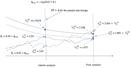
Suppose that the trial continues as planned without sample size change (hence no change in the final critical boundary). Suppose that at the final analysis, $({\hat{\theta }}_1,{\hat{\theta }}_2)=(0.22,0.24)$ were observed with common standard error $\mathit{s}.\mathit{e}.({\hat{\theta }}_1)=\mathit{s}.\mathit{e}.({\hat{\theta }}_2)=0.106$. Then $z_{1,2}^{(1)}=0.22/0.106=1.981$, $z_{2,2}^{\left(1\right)}=0.24/0.106=2.264$. Note that $z_{2,2}^{\left(1\right)}>{\hspace{0.17em}}_{\hspace{0.17em}}^2{c}_2^{\left(1\right)}=2.248088\mathit{\hspace{0.17em}}$, and $z_{2,2}^{\left(1\right)}>{\hspace{0.17em}}_{\hspace{0.17em}}^1{c}_2^{\left(1\right)}=1.977431$. Hence, level 2 hypothesis testing rejects the null hypothesis of $H_0^{\left(2\right)}=\cap \mathit{\hspace{0.17em}}\mathit{m}=12H_{0,\mathit{m}}$ : $\mathit{max}\left({\theta }_1,{\theta }_2\right)=0$. Since also $z_{2,2}^{\left(1\right)}>{\hspace{0.17em}}_{\hspace{0.17em}}^2{c}_2^{\left(1\right)}$, the level 1 test rejects the null hypothesis $H_{0,2}$ : ${\theta }_2=0$ as well. Since $z_1^{\left(1\right)}<{\hspace{0.17em}}_{\hspace{0.17em}}^2{c}_2$, $H_{0,1}$ : ${\theta }_1=0$ can’t be rejected with the level 2 test. However, since the null hypothesis of $H_0^{\left(2\right)}={\cap }_2^{m=1}{H}_{0,\mathit{m}}$ has been rejected by $z_{2,2}^{\left(1\right)}$, $z_1^{\left(1\right)}$ only needs to be compared with ${\hspace{0.17em}}_{\hspace{0.17em}}^1{c}_2$ per the closed testing procedure. Since $z_1^{\left(1\right)}>{\hspace{0.17em}}_{\hspace{0.17em}}^1{c}_2$, $H_{0,1}$ : ${\theta }_1=0$ is rejected. The rejection of $H_{0,1}$ would not be possible without the closed testing procedure. The $\mathit{p}$-value for the overall test (level 2) is $\mathit{p}=0.024$. The conservative point estimate for ${\theta }_{\mathit{max}}$ is $\hat{\theta }=0.1817$, and the conservative two-sided 95% confidence interval is (0.0017,0.4475) (see Figure 2 in the online supporting material). Note that because ${\hat{\theta }}_2=\mathit{max}({\hat{\theta }}_1,{\hat{\theta }}_2)$, it is assumed that ${\theta }_{\mathit{max}}={\theta }_2$. The estimate and confidence interval for ${\theta }_1$ needs to be calculated separately using the level 1 boundaries. Two imaginary curves of Wald statistics are used in Figure 2 for illustration. The two curves illustrate the trajectories of the Wald statistics $Z_i\left(\mathit{t}\right)=W_i\left(\mathit{t}\right)/\sqrt{\mathit{t}}$, $\mathit{i}=1,2$.

Figure 2. Scenario 2 illustration.

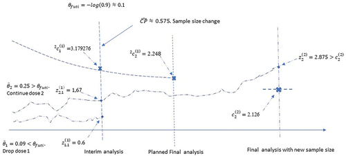
4.2.2. Scenario 2: sample size change and regimen dropping

Suppose that $({\hat{\theta }}_1,{\hat{\theta }}_2)=(0.09,0.25)$ are observed, with common standard error

$\mathit{s}.\mathit{e}.({\hat{\theta }}_1)=\mathit{s}.\mathit{e}.({\hat{\theta }}_2)=0.15$. Accordingly, $z_{1,1}^{(1)}=0.09/0.15=0.6$; and $z_{2,1}^{(1)}=0.25/0.15=1.67$. Since $z_{1,1}^{(1)}<{\hspace{0.17em}}_{\hspace{0.17em}}^2{c}_1^{(1)}=$3.179276 and $z_{2,1}^{(1)}<{\hspace{0.17em}}_{\hspace{0.17em}}^2{c}_1^{(1)}=$3.179276, the null hypothesis is not rejected. Also, since ${\hat{\theta }}_1<0.1$ and hence did not meet the criteria for clinically meaningful benefit, regimen 1 will be dropped from further enrollment. After dropping regimen 1, the conditional power with the planned sample size is 0.575. Sample size re-estimation suggests that the total number of events for the two remaining arms should increase to 374 (this number excludes the events in the dropped regimen before the interim analysis) to achieve a conditional power of 90%. No more interim analysis is planned except a final analysis. The new critical boundary for the final analysis is $c_2^{\left(2\right)}=$ 2.126. Suppose that at the final analysis, ${\hat{\theta }}_2=0.23$ were observed with standard error $\mathit{s}.\mathit{e}.\left({\hat{\theta }}_2\right)=0.08$. $z_2^{\left(2\right)}=0.23/0.08=2.875$. Hence the null hypothesis of $H_0^{\left(2\right)}=2\mathit{m}=1H_{0,\mathit{m}}$ : $\mathit{max}\left({\theta }_1,{\theta }_2\right)=0$ is rejected. Since regimen 1 has been dropped, this suggests that ${\theta }_2>0$. The final p-value is $\mathit{p}=0.005$.The point estimate and the conservative two-sided 95% confidence interval are ${\hat{\theta }}_2=0.1947$ (0.047616,0.393584). figure Two imaginary curves of Wald statistics are used in Figure 2 for illustration. The two curves illustrate the trajectories of the Wald statistics $Z_i\left(\mathit{t}\right)=W_i\left(\mathit{t}\right)/\sqrt{\mathit{t}}$, $\mathit{i}=1,2$.

5. Discussion

The properties of the score function are well known (Jennison and Turnbull 1997). It is approximately a Brownian motion. Because of this property, the multi-dimensional Markov process, formed by the vector of the score functions, is a precise mathematical model for describing the accumulative data for an MCSD/AMCSD procedure. The type I error is exact and sample size/power calculation is precise if the covariance matrix is known. In more general cases, the type error control, sample size/power calculation is conservative. In this sense, the procedure is optimally conservative. The method allows flexible decision rule for adaptive changes.

By utilizing Slepian’s lemma, the procedure can be applied to any distribution for which the score function is approximately a Brownian motion (e.g., Jennison and Turnbull 1997), such distributions include the normal distribution, binary distribution, survival analysis, Poisson distribution, and the negative binomial distribution. In a dose selection trial with a normal endpoint, the correlations between any two score functions can be derived as 0.5. For all other situations, the correlation is considered to be unknown, and Slepian’s lemma is applied, which conservatively assumes the correlation coefficients to be zero. All these distributions are supported by the DACT software. The procedure can be applied to a wide range of trials, including dose, treatment, end point selection, or a mixture of these selections. It can also be applied to population enrichment. To apply the procedure, $\mathit{M}$ score functions need to be created. Suppose that there are $\mathit{M}$ active doses/treatments in a dose/treatment selection trial, the comparison of each active dose/treatment arm with the control corresponds to a score function. In a trial that involves one active treatment arm and a control arm with $\mathit{M}$ endpoints, each endpoint corresponds to a score function. In a population enrichment trial that is randomized between an active treatment arm and a control arm, and in which a total of $\mathit{M}$ (sub) populations are considered, the comparison between the active treatment and the control for each subpopulation corresponds to a score function. Such an association between a comparison and a score function can be applied to a trial that involves a mixture of dose/treatment, endpoint. population enrichment comparison in the same manner. The method is complete in the sense that it includes sample size and power calculation, sample size re-estimation and it provides inference which includes point estimate, confidence interval and p-values.

Acknowledgements

The authors would like to thank the reviewers for helpful and constructive comments.

Disclosure statement

No potential conflict of interest was reported by the author(s).

Supplementary material

Supplemental data for this article can be accessed online at https://doi.org/10.1080/10543406.2023.2233590.

Additional information

Funding

The authors reported there is no funding associated with the work featured in this article.

References

- Armitage, P., C. K. McPherson, and B. C. Rowe. 1969. Repeated significance tests on accumulating data. Journal of the Royal Statistical Society (General) 132 (2):235–244.
- Bauer, P., F. Bretz, V. Dragalin, F. König, and G. Wassmer. Twenty-five years of confirmatory adaptive designs: Opportunities and pitfalls. Statistics in Medicine 35(3):325–347. 15 Mar 2015. doi:10.1002/sim.6472.
- Bretz, F., H. Schmidli, F. Knig, A. Racine, and W. Maurer. 2006. Confirmatory seamless phase II/III clinical trials with hypotheses selection at interim: General concepts. Biometrical Journal 48 (4):623–634. doi:10.1002/bimj.200510232.
- Chen, Y. H., D. L. DeMets, and K. K. G. Lan. 2010. Some drop-the-loser designs for monitoring multiple doses. Statistics in Medicine. 29(17):1793–1807. 10.1002/sim.3958.
- clinicaltrials.gov. A 3-arm multi-center, randomized controlled study comparing transforaminal corticosteroid, transforaminal etanercept and transforaminal saline for lumbosacral radiculopathy. https://clinicaltrials.gov/ct2/show/NCT00733096
- Dunnett, C. W. 1955. A multiple comparison procedure for comparing several treatments with a control. Journal of the American Statistical Association. 50 (272):1096–1121. doi:10.1080/01621459.1955.10501294.
- European medicines agency. 2020. Call to pool research resources into large multi-centre, multi-arm clinical trials to generate sound evidence on COVID-19 treatments. Media and Public Relations. (March 19).
- Freidlin, B., E. L. Korn, R. Gray, and A. Martin. Jul 15, 2008. Multi-arm clinical trials of new agents: Some design considerations. Clinical Cancer Research: An Official Journal of the American Association for Cancer Research 14 (14):4368–4371. doi:10.1158/1078-0432.CCR-08-0325.
- Gao, P., L. Y. Liu, and C. Mehta. 2013. Exact inference for adaptive group sequential designs. Statistics in Medicine 32 (23):3991–4005. 15 October 2013. doi:10.1002/sim.5847.
- Gao, P., L. Y. Liu, and C. Mehta. 2014. Adaptive sequential testing for multiple comparisons. Journal of Biopharmaceutical Statistics 24 (5):1035–1058. doi:10.1080/10543406.2014.931409.
- Gao, P., J. H. Ware, and C. Mehta. 2008. Sample size re-estimation for adaptive sequential designs. Journal of Biopharmaceutical Statistics 18 (6):1184–1196. 2008. doi:10.1080/10543400802369053.
- Ghosh, P., L. Y. Liu, P. Senchaudhuri, P. Gao, and C. Mehta. December 2017. Design and monitoring of multi-arm multi-stage clinical trials. Biometrics 73(4):1289–1299. doi: 10.1111/biom.12687.
- Hayter, A. J. 1986. The maximum familywise error rate of Fisher's least significant difference test. Journal of the American Statistical Association 81:1001–1004.
- Huffer, F. 1986. Slepian’s inequality via the central limit theorem. Canadian Journal of Statistics 367–370. doi:10.2307/3315195.
- Jaki, T., and L. V. Hampson. 2016. Designing multi-arm multi-stage clinical trials using a risk–benefit criterion for treatment selection. Statistics in Medicine 35 (4):522–533. doi:10.1002/sim.6760.
- Jaki, T., and J. M. S. Wason. Multi-arm multi-stage trials can improve the efficiency of finding effective treatments for stroke: A case study. BMC Cardiovascular Disorders 18(1):215. 2018 Nov 27. doi:10.1186/s12872-018-0956-4.
- Jennison, C., and B. W. Turnbull. 1997. Group sequential analysis incorporating covariance information. Journal of the American Statistical Association 92 (440):1330–1441. doi:10.1080/01621459.1997.10473654.
- Jennison, C., and B. W. Turnbull. 2000. Group sequential methods with applications to clinical trials. Boca Raton, FL: Chapman & Hall/CRC. doi:10.1201/9781584888581.
- Magirr, D., T. Jaki, and J. Whitehead. 2012. A generalized Dunnett test for multi-arm multi-stage clinical studies with treatment selection. Biometrika (2012) 99 (2):494–501. doi:10.1093/biomet/ass002.
- Marcus, R., E. Peritz, and K. R. Gabriel. 1976. On closed testing procedures with special reference to ordered analysis of variance. Biometrika 63 (3):655–660. doi:10.1093/biomet/63.3.655.
- Moore, T. J., H. Zhang, G. Anderson, and G. C. Alexander. 2018. Estimated costs of pivotal trials for novel therapeutic agents approved by the us food and drug administration, 2015-2016. JAMA Internal Medicine 178 (11):1451–1457. doi:10.1001/jamainternmed.2018.3931.
- National Institute of Health. n.d. The multi-arm optimization of stroke thrombosis. https://www.nihstrokenet.org/most/most
- O’Brien, P. C., and T. R. Fleming. Sep 1979. A multiple testing procedure for clinical trials. Biometrics 35(3):549–556. doi: 10.2307/2530245.
- Pocock, S. J. 1977. Group sequential methods in the design and analysis of clinical trials. Biometrika 64 (2):191–199. doi:10.1093/biomet/64.2.191.
- Slepian, D. 1962. The one-sided barrier problem for Gaussian Noise. Bell System Technical Journal 41 (2):463–501. doi:10.1002/j.1538-7305.1962.tb02419.x.
- Stallard, N., and T. Friede. 2008. A group-sequential design for clinical trials with treatment selection. Statistics in Medicine 27 (29):6209–6227. doi:10.1002/sim.3436.
- U.S. Department of Health and Human Services Food and Drug Administration (CDER and CBER). 2019. Enrichment strategies for clinical trials to support determination of effectiveness of human drugs and biological products guidance for industry. https://www.fda.gov/regulatory-information/search-fda-guidance-documents/enrichment-strategies-clinical-trials-support-approval-human-drugs-and-biological-products
- U.S. department of health and human services food and drug administration (CDER and CBER). 2019. Guidance for Industry Adaptive Design Clinical Trials for Drugs and Biologics.
- Wason, J., D. Magirr, M. Law, and T. Jaki. 2016. Some recommendations for multi-arm multi-stage trials. Statistical Methods in Medical Research 25 (2):716–727. doi:10.1177/0962280212465498.
- Wason, J., N. Stallard, J. Bowden, and C. Jennison. 2017. A multi-stage drop-the-losers design for multi-arm clinical trials. Statistical Methods in Medical Research 26 (1):508–524. doi:10.1177/0962280214550759.
- Whitehead, J. 1997. The design and analysis of sequential clinical trials. Rev. 2nd ed. England, West Sussex: John Wiley & Sons Ltd.