Adaptive sequential design for phase II single-arm oncology trials: an expansion of Simon’s design

ABSTRACT

Single-arm phase II trials are very common in oncology. A fixed sample trial may lack sufficient power if the true efficacy is less than the assumed one. Adaptive designs have been proposed in the literature. We propose a Simon’s design based, adaptive sequential design. Simon’s design is the most used fixed sample design for single-arm phase II oncology trials. A prominent feature of Simon’s design is that it minimizes the sample size when there is no clinically meaningful efficacy. We identify Simon’s trial as a special group sequential design. Established methods for sample size re-estimation (SSR) can be readily applied to Simon’s design. Simulations show that simply adding SSR to Simon’s design may still not provide desirable power. We propose some expansions to Simon’s design. The expanded design with SSR can provide even more power.

KEYWORDS:

• Oncology
• Simon’s design
• adaptive design
• sample size re-estimation
• score function

1. Introduction

In phase II single-arm trials, the primary endpoint is often a binary response rate $\mathit{p}$ (e.g., radiological response, tumor response rate, or objective response rate (ORR) (U.S. Food and Drug Administration, 2018). The null hypothesis is that the response rate does not exceed some $p_0$, which is a response rate indicating low activity with insufficient clinical benefit. The alternative hypothesis is that the response rate is larger than $p_0$. Clinical considerations may suggest some $p_{\mathit{low}}$ (which is larger than $p_0$) such that any response rate no less than $p_{\mathit{low}}$ will be clinically meaningful. The response rate $p_{\mathit{low}}$ will depend on the cancer type and available treatment options. For some recalcitrant cancer in patients with some specific genes with limited treatment options, even incremental efficacy (e.g., such as $p_{\mathit{low}}<0.2)$ can be clinically meaningful. With over 3500 citations, Simon’s two-stage design Simon (1989) is the most used design for single-arm phase II oncology trials. Simon’s designs are fixed sample designs. A fixed sample trial designed to provide $1-\mathit{\beta }$ power for $\mathit{p}=p_{\mathit{low}}$ will also provide at least $1-\mathit{\beta }$ power if the true response rate is larger. This is to say that there is a fixed sample size that can provide adequate power for a range of possible response rates. However, such a trial assumes the lowest clinically meaningful response rate and is the largest trial of all possibilities. The large sample size with this design is unnecessary if the true response rate is higher than $p_{\mathit{low}}$. Oncology trials are usually very expensive and time consuming, trials with potentially unnecessarily large sample sizes are often undesirable. An ideal sample size is such that it’s “just about right”, but determining accurate sample size requires precise knowledge about the true response rate which is often unknown. Usually, a target response rate $p_1>p_{\mathit{low}}$ is assumed (which may not be accurate for various reasons) for power calculation. However, the trial will be underpowered if the true response rate $\mathit{p}$ is smaller than the assumed $p_1$. Similar concerns about underpowered trial designs are also common in placebo-controlled studies and have motivated extensive research on sample size re-estimation (SSR), and such methods have been widely used (e.g., U.S Food and Drug Administration (CDER and CBER) (2019)) to provide flexibility in trial design. There are mainly two categories of such methods: combination tests/conditional error functions (e.g., Bauer and Kohne (1994); Proschan and Hunsberger (1995)), and adaptive sequential designs (ASD) (e.g., Cui et al. (1999); Müller and Schäfer (2001); Jennison and Turnbull (2003, 2006); Chen et al. (2004); Gao et al. (2008). Conditional error function-based methods for SSR have been proposed for phase II single-arm studies (e.g., Englert and Kieser 2012; Englert and S 2013; Kunzmann and Kieser 2016). In this article, we propose an ASD that can be used for single-arm trials. We show that Simon’s design is a special kind of group sequential design, and thus can be naturally combined with SSR methods from ASD Gao et al. (2008), and Gao et al. (2013). However, we also show through simulations that simply adding SSR to Simon’s design may not sufficiently increase the power. For this reason, we first augment and expand Simon’s design, all following Simon’s designing considerations. Then, we combine the expansions with SSR, which provides more power than Simon’s design combined with SSR. The method is an ASD and retains the basic structure and considerations of Simon’s design. Our design is mathematically similar to the sequential design by Chang et al. (1987), but our constraint on sample size is more aligned with that of Simon (1989). Like other two-stage designs Simon (1989); Jung et al. (2004); Lin and Shih (2004); Englert and Kieser (2012); Englert and S (2013), our method includes a first stage in which a futility analysis is conducted, and the trial is terminated if the efficacy does not reach a clinical meaningful threshold. If the trial is not stopped for futility, further patients are then enrolled to assess efficacy in the second stage. Our method also includes an option for three-stage design which is statistically more efficient. One feature of ASD-based SSR (used in our proposal) is that exact inference Gao et al. (2013) is available, which includes median unbiased estimate for efficacy, and two-sided exact confidence interval. Further, through simulations, we show that even with adaptive design, satisfactory operating characteristics (OC) (e.g., power and sample size) are not automatic. We provide several design options for the users to explore, compare, and choose from. We recommend that simulations be conducted to investigate the OCs of designs under consideration such that designs with desirable OCs can be selected. The proposed method and simulations are supported by the software Design and Analysis for Clinical Trials (DACT) at https://www.innovatiostat.com/softeware.html, which is free for academic researchers. Computing codes are provided in the online supporting material and also available upon request.

2. Simon’s design and challenges in phase II oncology trials

2.1. Notations

Simon’s design is a two-stage design which includes four parameters $r_1,n_1,r_2,n_2$. We propose several two-stage (the hybrid and the mid-point designs) and a three-stage design in this article, each of these will involve similar parameters. We introduce some notations to distinguish the designs and the associated parameters.

2.2. Simon’s design

Let $\mathit{p}$, $p_0$ and $p_1$ be as discussed above. Sample size is calculated assuming that the response rate is $p_1$. There are two stages in Simon’s design. In stage 1, $n_1$ subjects will be enrolled. If no more than $r_1$ responses are observed, then the trial would be stopped for futility. Otherwise, the trial proceeds to the second stage and enroll to a total of $n_2$ subjects for the trial. The null hypothesis will be rejected if more than $r_2$ responses are observed at the end of the trial. Let $\mathit{B}\left(\mathit{r},\mathit{p},\mathit{n}\right)$ denote the cumulative binomial distribution, and $\mathit{b}\left(\mathit{r},\mathit{p},\mathit{n}\right)$ the binomial probability mass function. Let $\mathrm{\Delta }{n}_{12}=n_2-n_1$. Let $\mathit{f}\left(r_1,n_1,r_2,n_2,\mathit{p}\right)=\mathit{B}\left(r_1,\mathit{p},n_1\right)+{\sum }_{x=r_1+1}^{\mathit{min}\left[n_1,r_2\right]}\mathit{b}\left(\mathit{x},\mathit{p},n_1\right)\mathit{B}\left(r_2-\mathit{x},\mathit{p},\mathrm{\Delta }{n}_{12}\right)$. This is the probability of not rejecting the null hypothesis with the response rate of $\mathit{p}$ (Simon, 1989). The type I error is $1-\mathit{f}\left(r_1,n_1,\mathit{r},n_2,p_0\mathit{\hspace{0.17em}}\right)$. The type II error and power are $\mathit{f}\left(r_1,n_1,\mathit{r},n_2,\mathit{p}\right)$ and $1-\mathit{f}\left(r_1,n_1,\mathit{r},n_2,\mathit{p}\right)$, respectively. $\mathit{PET}\left(\mathit{p}\right)=\mathit{B}\left(r_1;\mathit{p},n_1\right)$ is the probability of early termination. The expected sample size is $\mathit{EN}\left(\mathit{p}\right)=n_1+\left(1-\mathit{PET}\left(\mathit{p}\right)\right)\mathrm{\Delta }{n}_{12}$. A Simon’s design includes the quadruplet ($n_1$,$r_1$, $n_2$,$r_2$), such that under $p_0,\mathit{p},\mathit{\alpha },\mathit{\beta }$, the quadruplet satisfies the three considerations/constraints: i) The one-sided type I error should be controlled at a target level $\mathit{\alpha }$; ii) the type II error be controlled at $\mathit{\beta }$. iii) minimizing the sample size when the drug has no sufficient activity. We refer to these as Simon’s considerations. All methods for sample size calculation for clinical trials share the first two constraints/considerations. The third one aims to select the smallest $n_2$ under $p_0$ (among all possible quadruplets) for the minimax design, or the smallest $\mathit{EN}\left(p_0\right)$ for the optimal design Simon (1989). This is a distinctive feature for Simon’s design, and likely contributed to the huge popularity of Simon’s design. Let $\mathit{S}\left(p_0,\mathit{p},\mathit{\alpha },\mathit{\beta }\right)$ denote the quadruplet ($n_1$,$r_1$, $n_2$,$r_2$) under $p_0,\mathit{p},\mathit{\alpha },\mathit{\beta }$.

2.3. Group sequential design and Simon’s design

Let ${X_i}_{}\mathit{B}\left(\mathit{p}\right)$, $\mathit{i}=1,\dots ,\mathit{n}$ be random samples from a binary distribution with $\mathit{P}\left(X_i=1\right)=\mathit{p}$, and $\mathit{P}\left(X_i=0\right)=1-\mathit{p}$. The parameter of interest is $\mathit{\theta }=\mathit{p}-p_0$. Let $\hat{p}=\bar{X}=\frac{1}{n}{\sum }_{i=1}^n{X}_i$. Let $\mathit{s}.\mathit{e}.\left(\hat{p}\right)=\sqrt{\hat{p}\left(1-\hat{p}\right)/\mathit{n}}$ be the standard error for $\hat{p}$. $\hat{t}=\left[\mathit{s}.\mathit{e}.\left(\hat{p}\right)\right]{\mathit{\hspace{0.17em}}}^{-2}$ is the estimated Fisher’s information time. Then $\mathit{Z}\left(\mathit{\hspace{0.17em}}\hat{t}\right)=\left(\hat{p}-p_0\right)\sqrt{\hat{t}}\mathit{\hspace{0.17em}}$ is approximately $\mathit{N}\left(\mathit{\theta }\sqrt{\hat{t}},1\right)$ distributed and will be the Wald statistics from the observations $\left(X_1,\dots ,X_n\right)$.

Let the Fisher’s information times be $t_i=\frac{n_i}{\mathit{p}\left(1-\mathit{p}\right)}$, $\mathit{i}=1,2$, where $n_i$ is the sample size at the $\mathit{i}$-th stage analysis. Let $s_i=t_i/\mathit{T}$ be the information fractions, where $\mathit{T}=t_K$ is the total information time for the trial. Let $d_1=\left(\frac{r_1}{n_1}-p_0\right)\sqrt{\frac{{\left(n_1\right)}^3}{r_1\left(n_1-r_1\right)}}$, $c_1=+\mathrm{\infty }$, $c_2=\left(\frac{r_2}{n_2}-p_0\right)\sqrt{\frac{{\left(n_2\right)}^3}{r_2\left(n_2-r_2\right)}}$. Let $x_i$be the number of observed responses at $n_i$, $\mathit{i}=1,2$. In Simon’s design the trial is terminated for futility at $n_1$ if $\left(x_1\le r_1\right)$ is observed, and the null hypothesis of $\mathit{p}\le p_0$ is rejected if $\left(x_2\ge r_2\right)$ is observed at $n_2$. Let ${\hat{t}}_{\mathit{i}}=\left[\mathit{s}.\mathit{e}.\left(\mathit{\hspace{0.17em}}\hat{p}\right)\right]{\mathit{\hspace{0.17em}}}^{-2}$ $=n_i{\left[\frac{x_i}{n_i}\left(1-\frac{x_i}{n_i}\right)\right]}^{-1}=\frac{{\left(n_i\right)}^3}{x_i\left(n_i-x_i\right)}$ be the estimated Fisher’s information time at $n_i$. Let $\mathit{Z}\left(t_i\right)=\left(\frac{x_i}{n_i}-p_0\right)\times \sqrt{\mathit{\hspace{0.17em}}{\hat{t}}_{\mathit{i}}}$. Then $\left(x_1\le r_1\right)$is the same event as $\left(\mathit{Z}\left(t_1\right)\le \mathit{\hspace{0.17em}}{d}_1\right)$, and $\left(x_2\ge r_2\right)$ is the same event as $\left(\mathit{Z}\left(t_2\right)\ge \mathit{\hspace{0.17em}}{c}_2\right)$. i.e., Simon’s design is a GSD, such that the trial is terminated for futility if $\left(\mathit{Z}\left(t_1\right)\le \mathit{\hspace{0.17em}}{d}_1\right)$ is observed, and the null hypothesis rejected if $\left(\mathit{Z}\left(t_2\right)\ge \mathit{\hspace{0.17em}}{c}_2\right)$ is observed. GSD are commonly designed by deriving critical boundaries such as O’Brien-Fleming boundary O’Brien and Fleming (1979), the Pocock (1977), or $\mathit{\alpha }$- spending Lan and DeMets (1983) at planned information fractions to control type I error, while the boundaries $d_1$ and $c_2$ in Simon’s design are derived from ($n_1$,$r_1$, $n_2$,$r_2$) and $p_0$. $d_1$ and $c_2$ properly control type I error because ($n_1$,$r_1$, $n_2$,$r_2$) does.

Pocock’s boundaries satisfy $c_1=c_2$, and O’Brien-Fleming boundaries satisfy $c_1\sqrt{t_1}=c_2\sqrt{t_2}$. The motivation for Simon’s design is different from both Pocock’s and O’Brien-Fleming boundaries. Hence, the boundaries are naturally different, with $c_1=+\mathrm{\infty }$ in Simon’s design.

2.4. Challenges in phase II oncology trials and the need for SSR

A fixed sample design, including Simon’s design, provides adequate power only when the true response rate is no less than the assumed response rate $p_1$. The power will be less than $1-\mathit{\beta }$ if the true response rate is less than $p_1$. In practice, a range of response rates can be clinically beneficial. Besides $p_{\mathit{low}}$, prior clinical evidence, or pathological analysis and mode of action may suggest that some optimistic response rate $p_{\mathit{high}}$may be possible. Any assumed response rate is reasonable if it is between $p_{\mathit{low}}\mathit{\hspace{0.17em}}$ and $p_{\mathit{high}}$. A flexible design is such that it targets some response rate $p_1$between $p_{\mathit{low}}$ and $p_{\mathit{high}}$, and with a sample size smaller than $n_2^{Si\mathrm{mon}}\left(p_0,p_{\mathit{low}}\right)$, but allows for sample size increase to that similar to $n_2^{Si\mathrm{mon}}\left(p_0,\hat{p}\right)$, if the observed response rate is $\hat{p}$ at the interim analysis, with $p_{\mathit{low}}<\mathit{\hspace{0.17em}}\hat{p}\mathit{\hspace{0.17em}}<p_1$. We have identified that Simon’s design is a special type of group sequential design. Hence, it is natural to utilize and combine available methods in ASD with Simon’s design.

3. Adaptive sequential design with binding futility termination boundary

An ASD is the combination of a group sequential design (GSD) with adaptive features such as sample size modification. The first step in an ASD is to select a GSD. Let $\mathit{\theta }$ be the efficacy parameter, larger values of $\mathit{\theta }$ indicates better efficacy. Let the null hypothesis $H_0$ be that $\mathit{\theta }\le 0$, and the one-sided alternative hypothesis $H_a$ be that $\mathit{\theta }>0$. In a GSD, $\mathit{K}$ (including interim and the final) analyses will be conducted at information times $0<t_1<\dots <t_K$. Let $Z_i$ be the Wald statistics at the $\mathit{i}$-th interim analysis. Critical boundaries $c_1,\dots ,c_K$ and futility boundaries $d_1,\dots ,d_{\mathit{K}-1}$ may be selected, such that the null hypothesis $H_0$ is rejected if $Z_i\ge c_i$ is observed at any $1\le \mathit{i}\le \mathit{K}$, and the trial declared futile and terminated if the $Z_i<d_i$ is observed for any $1\le \mathit{i}\le \mathit{K}-1$. The $c_i$’s and $d_i$’s are chosen such that the one-sided type I error is controlled at level $\mathit{\alpha }$. The futility boundaries $d_1,\dots ,d_{\mathit{K}-1}$ can be chosen to be either binding or non-binding. If the Wald statistics for single-arm trials can be constructed, then the usual GSD can be applied to single-arm trials, in a completely parallel manner.

3.1. Applying sample size re-estimation to Simon’s design

3.1.1. The SSR algorithm

SSR procedure can be used to increase sample size when the observed effect size is smaller than the assumed. The SSR procedure in a single arm oncology trial can be completely parallel to that in ASD (e.g., Cui et al. (1999); Müller and Schäfer (2001); Gao et al. (2008) for two arm comparison. Let $\hat{p}$ be the MLE of $\mathit{p}$ at the interim analysis with a sample size of $n_1$. Then the conditional power of rejecting the null hypothesis at the end of the trial with planned sample size $n_2$ Gao et al. (2008) is $\mathit{c}{p}_{n_2}=\mathit{P}\left(\mathit{Z}\left(\mathit{\hspace{0.17em}}{t}_2\right)\ge c_2|\mathit{Z}\left(\mathit{\hspace{0.17em}}{t}_1\right)=z_1\right)=\mathrm{\Phi }\left(\left(p_1-p_0\right)\sqrt{t_2-t_1}-\frac{c_2\sqrt{t_2}-\mathit{Z}\left(\mathit{\hspace{0.17em}}{t}_1\right)\sqrt{t_1}}{\sqrt{t_2-t_1}}\right)$. And the estimated conditional power is ${\widehat{\mathit{cp}}}_{n_2}=\mathrm{\Phi }\left(\left(\hat{p}-p_0\right)\sqrt{{\hat{t}}_2-{\hat{t}}_1}-\frac{c_2\sqrt{{\hat{t}}_2}-\mathit{Z}\left({\hat{t}}_1\right)\sqrt{{\hat{t}}_1}}{\sqrt{{\hat{t}}_2-{\hat{t}}_1}}\right)$, where ${\hat{t}}_2={\hat{t}}_1\times n_2\mathit{\hspace{0.17em}}/n_1$. If ${\widehat{\mathit{cp}}}_{n_2}<1-\mathit{\beta }$, then the sample size may be increased to $n_{\mathit{new}}$, such that ${\widehat{\mathit{cp}}}_{n_{\mathit{ew}}}\ge 1-\mathit{\beta }$, where ${\widehat{\mathit{cp}}}_{n_{\mathit{ew}}}=\mathrm{\Phi }\left(\left(\hat{p}-p_0\right)\sqrt{{\hat{t}}_{\mathit{new},\left(1-\mathit{\beta }\right)}-{\hat{t}}_1}-\frac{c_2\sqrt{{\hat{t}}_2}-\mathit{Z}\left({\hat{t}}_1\right)\sqrt{{\hat{t}}_1}}{\sqrt{{\hat{t}}_2-{\hat{t}}_1}}\right)$ . ${\hat{t}}_{\mathit{new},\left(1-\mathit{\beta }\right)}$ can be solved Gao et al. (2008) as:

(1) ${\hat{t}}_{\mathit{new},\left(1-\mathit{\beta }\right)}\mathit{\hspace{0.17em}}\ge \frac{1}{{\left(\hat{p}-p_0\right)}^2}{\left\{{\mathrm{\Phi }}^{-1}\left(1-\mathit{\beta }\right)+\frac{c_2\sqrt{{\hat{t}}_2}-\mathit{Z}\left({\hat{t}}_1\right)\sqrt{{\hat{t}}_1}}{\sqrt{{\hat{t}}_2-{\hat{t}}_1}}\right\}}^2+{\hat{t}}_1$(1)

Let $n_{\mathit{new},\left(1-\mathit{\beta }\right)}=\hat{p}\left(1-\hat{p}\right)\times {\hat{t}}_{\mathit{new},\left(1-\mathit{\beta }\right)}$. Let $N_{\mathit{max}}$ be a pre-determined maximum feasible sample size. Then the new sample size may be chosen as $n_{\mathit{new}}=\mathit{min}\left(N_{\mathit{max}},n_{\mathit{new},\left(1-\mathit{\beta }\right)}\right)$. Let ${\hat{t}}_{\mathit{new}}={\hat{t}}_2\times n_{\mathit{new}}/n_2$. The final critical boundary at $n_{\mathit{new}}$ will be (see Gao et al. (2008)) $c_{\mathit{new}}=e_{\mathit{new}}/\sqrt{{\hat{t}}_{\mathit{new}}}$, where

(2) $e_{\mathit{new}}=\frac{\sqrt{{\hat{t}}_{\mathit{new}}-\mathit{\hspace{0.17em}}{\hat{t}}_1}}{\sqrt{{\hat{t}}_2-\mathit{\hspace{0.17em}}{\hat{t}}_1}}\left(c_2\sqrt{{\hat{t}}_2}-\mathit{Z}\left({\hat{t}}_1\right)\sqrt{{\hat{t}}_1}\right)+\mathit{Z}\left({\hat{t}}_1\right)\sqrt{{\hat{t}}_1}$(2)

Let $x_{\mathit{new}}$ be the number of responses observed at the final analysis. Let $r_{\mathit{new}}$ be the smallest integer such that

(3) $\left(\frac{{\mathit{r}}_{\mathit{new}}\mathit{\hspace{0.17em}}}{n_{\mathit{new}}}-p_0\right)\sqrt{\frac{{\left({\mathit{n}}_{\mathit{new}}\right)}^3}{r_{\mathit{new}}\mathit{\hspace{0.17em}}\left(n_{\mathit{new}}-r_{\mathit{new}}\mathit{\hspace{0.17em}}\right)}}\ge c_{\mathit{new}}.$(3)

Then the null hypothesis is rejected if $x_{\mathit{new}}\ge r_{\mathit{new}}$.

3.1.2. SSR using continuity correction

Due to the discreteness of the binary distribution, the above procedure for calculating $c_{\mathit{new}}$ may not exactly control the type I error and a continuity correction (e.g., Feller (1945); Devore (1995)) may need to be used. Let $r_i^{cor}$ $=$ $r_i+$0.5, $\mathit{i}=1,2$ be the continuity corrections for $r_i$. Let the continuity corrected binding futility boundary be $d_1^{cor}=\left(\frac{r_1^{cor}}{n_1}-p_0\right)\sqrt{\frac{{\left(n_1\right)}^3}{r_1^{cor}\left(n_1-r_1^{cor}\right)}}$, and $r_2^{cor}$ correspond to critical boundaries $c_2^{cor}=\left(\frac{{\mathit{r}}_{2,\mathit{cor}}}{n_2}-p_0\right)\sqrt{\frac{{\left(n_2\right)}^3}{r_2^{cor}\left(n_2-r_2^{cor}\right)}}$. Then $c_2^{cor}$ (instead of $c_2$) can be used to calculate $c_{new}^{cor}$ in the SSR, and $r_{new}^{cor}$ can be obtained in the same way as for $r_{\mathit{new}}$. Figure 1 demonstrates how to conduct interim analysis using DACT. DACT output includes $n_{\mathit{new}}$, $r_{\mathit{new}}$ and $r_{new}^{cor}$.

Figure 1. Interim analysis using DACT.

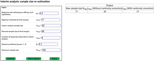
The interim analysis shown in Figure 1 can accommodate both the two-stage and the three-stage design (see section 3.2.4 on expansions). The sample size re-estimation is conducted at $n_1$ for a two-stage design and at $n_2$ for a three-stage design. Therefore, for a two-stage design, $n_{\mathit{inter}}=n_1$, $x_{\mathit{inter}}=x_1$, $n_{\mathit{final}}=n_2$, and $r_{\mathit{final}}=r_2$. For a three-stage design, $n_{\mathit{inter}}=n_2$, $x_{\mathit{inter}}=x_2$, $n_{\mathit{final}}=n_3$, and $r_{\mathit{final}}=r_3$. For the input in Figure 1, $r_{\mathit{new}}\ne r_{new}^{cor}$. However, if $x_{\mathit{inter}}$ is changed to 7, then $r_{\mathit{new}}=r_{new}^{cor}=15$.

The corrections $r_i^{cor},$ $\mathit{i}=1,2$ changes the calculations of $d_1^{cor}$ and $c_2^{cor}$, which superficially changes the sequential design, but they do not actually change the original two-stage design, because it is discrete. The continuity correction only affects the calculation of $c_{new}^{cor}$ in the SSR. $c_{new}^{cor}$ is calculated using formulas (1) and (2), with $c_2$ being replaced by $r_2^{cor}$. Then, $r_{new}^{cor}$ is identified using formula (3) with $n_{\mathit{new}}$ and $c_{\mathit{new}}$ being replaced by $n_{new}^{cor}$ and $c_{new}^{cor}$, respectively. So $r_1^{cor}$ is actually not used in this calculation and its definition is actually not necessary. But not defining $r_1^{cor}$ may invite questions which will also need explanations and keeping the definition of $r_1^{cor}$ may be a simpler approach. Per formula (1) and (2), $c_{new}^{cor}$ is affected by ${\hat{t}}_1$, ${\hat{t}}_2$ (which are determined by $n_1$, $n_2$), $\mathit{Z}\left({\hat{t}}_1\right)$ (which is affected by the number of observed responses), $r_2^{cor}$. None of these parameters are associated with the original design (i.e., optimal, minimax, or the expanded design [see section 3.1] such as the average, the hybrid. The midpoint, or the three-stage design).

The use of $c_2^{cor}$ may not always be necessary. The necessity may be checked with simulations. If the simulated type I error using $c_2$ is less than $\mathit{\alpha }$, the continuity correction would not be necessary. The simulations can be conducted using the DACT software, as illustrated in Figures 2 and 3.

Figure 2. Necessity of continuity correction in a two-stage design.

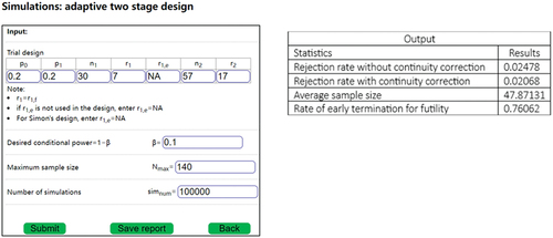
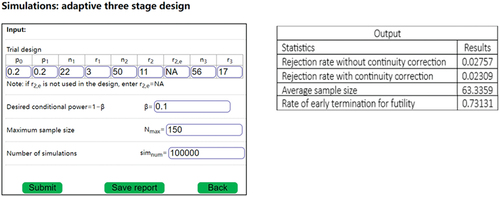
Figure 3. Necessity of continuity correction in a three-stage design.

In Figure 2, the type I error without continuity correction is <0.025, hence there is no need for the continuity correction.

In Figure 3, the type I error without continuity correction is >0.025, while the type I error is <0.025, hence continuity correction is necessary.

3.2. Expanding Simon’s design

3.2.1. Motivation for expanding Simon’s design

Combining an SSR procedure with Simon’s design, as discussed in the previous section, will add flexibility to Simon’s design and increase the power when the true response rate is lower than the assumed one. However, simulations (Table 4) show that simply adding the SSR procedure to $\mathit{S}\left(p_0,p_1,\mathit{\alpha },\mathit{\beta }\right)$ may still fall short of providing desired power when $\mathit{p}$ is close to $p_{\mathit{low}}$. One of the reasons is that $n_1^{Si\mathrm{mon}}\left(p_0,p_1\right)$ may be too small and that the related $\mathit{PET}\left(p_{\mathit{low}}\right)$ can be too large. To design a trial that can provide power of about $1-\mathit{\beta }$ for all $\mathit{p}$ between $p_{\mathit{low}}$ and $p_1$, changes must be made on Simon’s design. We seek to expand Simon’s design such that the expanded design is flexible and can satisfy Simon’s considerations for all $\mathit{p}$ between $p_{\mathit{low}}$ and $p_1$. Let $\mathit{E}{N}^{\mathit{Simon}}\left(p_0,p_{\mathit{low}}\right)$, $\mathit{E}{N}^{\mathit{Simon}}\left(p_0,p_1\right)$, $n_2^{Si\mathrm{mon}}\left(p_0,p_1\right)$ and $n_2^{Si\mathrm{mon}}\left(p_0,p_{\mathit{low}}\right)$ be defined as in Table 1. Because both $p_1$ and $p_{\mathit{low}}$ are among possible response rates, the trial designers could choose either $\mathit{S}\left(p_0,p_{\mathit{low}},\mathit{\alpha },\mathit{\beta }\right)$ or $\mathit{S}\left(p_0,p_1,\mathit{\alpha },\mathit{\beta }\right)$, and both are reasonable designs. Hence $\mathit{E}{N}^{\mathit{Simon}}\left(p_0,p_1\right)$, $\mathit{E}{N}^{\mathit{Simon}}\left(p_0,p_{\mathit{low}}\right)$ and $n_2^{Si\mathrm{mon}}\left(p_0,p_1\right)$ and $n_2^{Si\mathrm{mon}}\left(p_0,p_{\mathit{low}}\right)$ are all acceptable under Simon’s third consideration, and can be considered to be benchmarks, such that the $\mathit{EN}\left(p_0\right)$ or $n_2$ for the new design is permissible if it is no larger than $\mathit{E}{N}^{\mathit{Simon}}\left(p_0,p_{\mathit{low}}\right)$ or $n_2^{Si\mathrm{mon}}\left(p_0,p_{\mathit{low}}\right)$, respectively. Hence, the expansions will be permissible if $\mathit{EN}\left(p_0\right)$ or $n_2$ for the new designs are permissible. Trial designs with smaller $\mathit{EN}\left(p_0\right)$ or $n_2$ (i.e., closer to $\mathit{E}{N}^{\mathit{Simon}}\left(p_0,p_1\right)$ or $n_2^{Si\mathrm{mon}}\left(p_0,p_1\right)$, respectively) are preferable. Our motivation is to identify designs with permissible $\mathit{EN}\left(p_0\right)$ and $n_2$, and that they are as close to $\mathit{E}{N}^{\mathit{Simon}}\left(p_0,p_1\right)$ or $n_2^{Si\mathrm{mon}:}\left(p_0,p_1\right)$ as possible. Let $\mathit{PET}\left(p_{\mathit{low}}\right)$ be the probability of early futility termination under $\mathit{p}=p_{\mathit{low}}$ for a design. The power of combining SSR to a design will not exceed $1-\mathit{PET}\left(\mathit{p}\right)$, no matter the method is the combination test/conditional error function-based SSR (e.g., Englert and Kieser (2012); Englert and S (2013)), or an ASD method (such as proposed in this article). In order to achieve a power of $1-\mathit{\beta }$ when $\mathit{p}$ is close to $p_{\mathit{low}}$, $\mathit{PET}\left(p_{\mathit{low}}\right)<\mathit{\beta }$ must be required for the design. For $\mathit{S}\left(p_0,p_{\mathit{low}},\mathit{\alpha },\mathit{\beta }\right)$, $\mathit{PET}\left(p_{\mathit{low}}\right)=\mathit{B}\left(r_1,p_{\mathit{low}},n_1\right)<\mathit{\beta }$ is automatically satisfied. But for $\mathit{S}\left(p_0,p_1,\mathit{\alpha },\mathit{\beta }\right)$, it is possible that $\mathit{PET}\left(p_{\mathit{low}}\right)=\mathit{B}\left(r_1,p_{\mathit{low}},n_1^{Si\mathrm{mon}}\left(p_0,p_1\right)\mathit{\hspace{0.17em}}\right)>\mathit{\beta }$. When this happens, simply applying SSR to $\mathit{S}\left(p_0,p_1,\mathit{\alpha },\mathit{\beta }\right)$ will not provide desired power when $\mathit{p}$ is close to $p_{\mathit{low}}$. Applying SSR to $\mathit{S}\left(p_0,p_{\mathit{low}},\mathit{\alpha },\mathit{\beta }\right)$ won’t be necessary since the design already has enough power for all response rate no less than $p_{\mathit{low}}$. A suitable design would likely have a sample size between those for $\mathit{S}\left(p_0,p_1,\mathit{\alpha },\mathit{\beta }\right)$ and $\mathit{S}\left(p_0,p_{\mathit{low}},\mathit{\alpha },\mathit{\beta }\right)$. We propose several expansion options, which will be different compromises between $\mathit{S}\left(p_0,p_1,\mathit{\alpha },\mathit{\beta }\right)$ and $\mathit{S}\left(p_0,p_{\mathit{low}},\mathit{\alpha },\mathit{\beta }\right)$. Each will have a planned sample size smaller than $\mathit{S}\left(p_0,p_{\mathit{low}},\mathit{\alpha },\mathit{\beta }\right)$, but with SSR, can provide more power than that of $\mathit{S}\left(p_0,p_1,\mathit{\alpha },\mathit{\beta }\right)$ combined with SSR. Each of the expansions will satisfy Simon’s considerations, and that $\mathit{PET}\left(p_{\mathit{low}}\right)<\mathit{\beta }$. The last condition means that the sample sizes will need to be larger than that for $\mathit{S}\left(p_0,p_1,\mathit{\alpha },\mathit{\beta }\right)$. The expansions include a hybrid design, a midpoint design, and a three-stage design. However, before these expansions, we propose an average design, which is an augmentation of Simon’s optimal and minimax designs, but not an expansion. In Simon’s design, $r_1$ is a futility cutoff and will be denoted as $r_{1,\mathit{f}}$. While $r_2$ is an efficacy cutoff and will be denoted as $r_{2,\mathit{e}}$. In our expansions, we’ll denote futility cutoffs $r_i$ as $r_{\mathit{i},\mathit{f}}$, and efficacy cutoffs $r_i$ as $r_{\mathit{i},\mathit{e}}$.

Table 1. Notations.

Parameters	Notations
	Simon’s design	The hybrid design		The midpoint design	The three-stage design
Design	$\mathit{S}\left(p_0,\mathit{p},\mathit{\alpha },\mathit{\beta }\right)$
$r_1$	$r_1^{Si\mathrm{mon}:opt}\left(p_0,\mathit{p}\right)$	$r_1^{hy\mathrm{brid}}$		$r_1^{mi\mathrm{dpoint}}$	$r_1^{3-st\mathrm{age}}$
$r_{1,\mathit{f}}$		$r_{1,f}^{hy\mathrm{brid}}$		$r_{1,f}^{mi\mathrm{dpoint}}$	$r_{1,f}^{3-st\mathrm{age}}$
$r_{1,\mathit{e}}$		$r_{1,e}^{hy\mathrm{brid}}$		$r_{1,e}^{mi\mathrm{dpoint}}$	$r_{1,e}^{3-st\mathrm{age}}$
$n_1$	$n_1^{Si\mathrm{mon}:opt}\left(p_0,\mathit{p}\right)$	$n_1^{hy\mathrm{brid}}$		$n_1^{mi\mathrm{dpoint}}$	$n_1^{3-st\mathrm{age}}$
$r_2$	$r_2^{Si\mathrm{mon}:opt}1\left(p_0,\mathit{p}\right)$	$r_2^{hy\mathrm{brid}}$		$r_2^{mi\mathrm{dpoint}}$	$r_2^{3-st\mathrm{age}}$
$r_{2,\mathit{f}}$		$r_{2,f}^{hy\mathrm{brid}}$		$r_{2,f}^{mi\mathrm{dpoint}}$	$r_{2,f}^{3-st\mathrm{age}}$
$r_{2,\mathit{e}}$		$r_{2,e}^{hy\mathrm{brid}}$		$r_{2,e}^{mi\mathrm{dpoint}}$	$r_{2,e}^{3-st\mathrm{age}}$
$n_2$	$n_2^{Si\mathrm{mon}:opt}\left(p_0,\mathit{p}\right)$	$n_2^{hy\mathrm{brid}}$		$n_2^{mi\mathrm{dpoint}}$	$n_2^{3-st\mathrm{age}}$
$\mathit{PET}\left(\mathit{p}\right)$	$\mathit{PE}{T}^{\mathit{Simon}}\left(p_0,\mathit{p}\right)$	$\mathit{PE}{T}^{\mathit{hybrid}}\left(p_0\right)$		$\mathit{PE}{T}^{\mathit{midpoint}}\left(p_0\right)$	$\mathit{PE}{T}^{3-\mathit{stage}}\left(p_0\right)$
$\mathit{E}\left(p_0\right)$	$\mathit{E}{N}^{\mathit{Simon}}\left(p_0,\mathit{p}\right)$	$\mathit{E}{N}^{\mathit{hybrid}}\left(p_0\right)$		$\mathit{E}{N}^{\mathit{midpoint}}\left(p_0\right)$	$\mathit{E}{N}^{3-\mathit{stage}}\left(p_0\right)$
$n_1$: stage 1 sample size $r_1$: stage 1 futility criterion $r_{1,\mathit{f}}$: stage 1 futility criterion $r_{1,\mathit{e}}$: stage 1 efficacy criterion $n_2$: Sample size at end of stage 2 $r_2$: stage 2 efficacy criterion in a two-stage design			$r_{2,\mathit{e}}$: stage 2 efficacy criterion $n_3$: Sample size at end of stage 3$r_{2,\mathit{f}}$: stage 2 futility criterion $r_3$: stage 3 efficacy criterion $r_1^{Si\mathrm{mon}:opt}\left(p_0,\mathit{p}\right),\mathit{or}{r}_1^{Si\mathrm{mon}:mi\mathrm{nimax}}\left(p_0,\mathit{p}\right)$ means the $r_1$ from the optimal or minimax design

3.2.2. The average design – an augmentation

Jung et al. (2004) noted that “the two Simon’s designs may result in highly divergent sample size requirements”. Indeed, for example, if $p_0=0.2$, $p_1=0.33$, $\mathit{\alpha }=0.025$, $\mathit{\beta }=0.1$, then $n_1^{Si\mathrm{mon}:mi\mathrm{nimax}}\left(p_0,p_1\right)=100$, $n_2^{Si\mathrm{mon}:mi\mathrm{nimax}}\left(p_0,p_1\right)=119$ for the minimax design and $n_1^{Si\mathrm{mon}:opt}\left(p_0,p_1\right)=50$, $n_2^{Si\mathrm{mon}:opt}\left(p_0,p_1\right)=137$ for optimal design. Such divergence could present challenges for the trial designers, and also suggest that some other designs may also be reasonable choices. Jung et al. (2004) proposed the admissible designs. We propose an additional design option, the average design, to balance the desire to minimize the $\mathit{EN}\left(p_0\right)$(the optimal design) and that to minimize the $n_2$ (the minimax design). The optimal and the minimax designs will be derived first. Let $n_{1,\mathit{avg}}$, $r_{1,\mathit{avg}}$ be the smallest integers larger than the average of $n_1$’s and $r_1$’s from the optimal and minimax designs, respectively. Then search for $\left(n_2,r_2\right)$’s that satisfy $\mathit{f}\left(r_{1,\mathit{avg}},n_{1,\mathit{avg}},r_2,n_2,p_1\right)\le \mathit{\beta }$, and $1-\mathit{f}\left(r_{1,\mathit{avg}},n_{1,\mathit{avg}},r_2,n_2,p_0\right)\le \mathit{\alpha }$. $\left(\mathrm{\Delta }{n}_{12},r_2\right)$ can be chosen such that $\mathrm{\Delta }{n}_{12}$ is the smallest integer satisfying the requirement on type I and type II errors. Design examples are given in Table 2. The $n_2$ and $\mathit{EN}\left(p_0\right)$ for the average design are smaller than $n_2^{Si\mathrm{mon}:opt}\left(p_0,p_1\right)$, and $\mathit{E}{N}^{\mathit{Simon}:\mathit{minimax}}\left(p_0\right)$, respectively. Jung’s admissible designs aim to achieve the minimum of weighted average of $n_2$ (with weight $\mathit{q}$) and $\mathit{EN}\left(p_0\right)$ (with weight $1-\mathit{q}$), while the average design balances the desire for the smallest $n_2$ and the smallest $\mathit{EN}\left(p_0\right)$. Hence, the motivation of the average design is similar to Jung’s admissible design with $\mathit{q}=0.5$. However, they are obtained through different search processes, and thus are not expected to be exactly the same. The average design offers an additional option for trial designers when the minimax design and the optimal design are very different. Three admissible designs from Jung et al. (2004, Tables 1 and 2) are presented in Table 2 for comparison with the average design.

Table 2. Comparing the average design and Jung’s admissible design.

$\left(p_0,p_1,\mathit{\alpha },\mathit{\beta }\right)=\left(0.1,\mathit{\hspace{0.17em}}0.3,\mathit{\hspace{0.17em}}0.05,\mathit{\hspace{0.17em}}0.15\right)$
	$r_1$	$n_1$	$r_2$	$n_2$	$\mathit{err}$	$\mathit{EN}\left(p_0\right)$	$\mathit{PW}\left(p_1\right)$
minimax	2	18	5	27	0.0444	20.4	0.851
optimal	1	11	6	35	0.0422	18.3	0.851
Average	2	15	6	36	0.0433	18.9	0.852
Jung’s admissible	1	13	5	28	0.0498	18.7	0.858
$\left(p_0,p_1,\mathit{\alpha },\mathit{\beta }\right)=\left(0.05,\mathit{\hspace{0.17em}}0.25,\mathit{\hspace{0.17em}}0.05,\mathit{\hspace{0.17em}}0.1\right)$
	$r_1$	$n_1$	$r_2$	$n_2$	$\mathit{err}$	$\mathit{EN}\left(p_0\right)$	$\mathit{PW}\left(p_1\right)$
minimax	0	15	3	25	0.0336	20.4	0.901
optimal	0	9	3	30	0.0489	16.8	0.902
Average	0	12	3	26	0.0365	18.4	0.905
Jung’s admissible 1	0	12	3	26	0.0365	18.4	0.905
Jung’s admissible 2	0	10	3	28	0.0426	17.2	0.906

In Table 2, in the case of $\left(p_0,p_1,\mathit{\alpha },\mathit{\beta }\right)=\left(0.1,\mathit{\hspace{0.17em}}0.3,\mathit{\hspace{0.17em}}0.05,\mathit{\hspace{0.17em}}0.15\right)$, the average design is different form Jung’s admissible design. In the case of $\left(p_0,p_1,\mathit{\alpha },\mathit{\beta }\right)=\left(0.05,\mathit{\hspace{0.17em}}0.25,\mathit{\hspace{0.17em}}0.05,\mathit{\hspace{0.17em}}0.1\right)$, there are two Jung’s admissible designs, and one of them is the same as the average design.

3.2.3. The modified Simon’s design

Because of the necessity of achieving $\mathit{PET}\left(p_{\mathit{low}}\right)<\mathit{\beta }$, it is natural to think about modifying Simon’s design, by adding this constraint to Simon’s considerations in the search of the quadruplet $r_1,n_1,r_2,n_2$ for the two-stage design, such that the following will be satisfied: i) the type I error satisfies $\mathit{P}=1-\mathit{f}\left(r_1,n_1,\mathit{r},n_2,p_0\mathit{\hspace{0.17em}}\right)<\mathit{\alpha }$. ii) The power under $\mathit{p}=p_1$ satisfies $1-\mathit{f}\left(r_1,n_1,\mathit{r},n_2,p_1\right)\ge 1-$ $\mathit{\beta }$. iii) $\mathit{PET}\left(p_{\mathit{low}}\right)=\mathit{B}\left(r_1,p_{\mathit{low}},n_1\right)<\mathit{\beta }$. Similar to Simon’s design, among all the quadruplets that satisfy these constraints, the one with the smallest $n_2$ will be selected as the minimax design, and the one with the minimum $\mathit{EN}\left(p_0\right)$ will be the optimal design. However, our investigation shows that the requirement of $\mathit{PET}\left(p_{\mathit{low}}\right)=\mathit{B}\left(r_1,p_{\mathit{low}},n_1\right)<\mathit{\beta }$ frequently led to the reduction of $r_1$, and the difference between the modified design and the original Simon’s design is often minor. Consequently, the modified design combined with SSR may not meaningfully improve the power of the original Simon’s design $\mathit{S}\left(p_0,p_1,\mathit{\alpha },\mathit{\beta }\right)$ combined with SSR if the true response rate is close to $p_{\mathit{low}}$. Hence, the modified design will not be further discussed.

3.2.4. The expansions

Our investigation further shows that besides the requirement that $\mathit{PET}\left(p_{\mathit{low}}\right)<\mathit{\beta }$, $n_1$ (at which the SSR will be performed) can have significant impact on the power of a design combined with SSR. In order for a two-stage design plus SSR to have substantial power increase over Simon’s original design $\mathit{S}\left(p_0,p_1,\mathit{\alpha },\mathit{\beta }\right)$ plus SSR, $n_1$ will need to be larger than $n_1^{Si\mathrm{mon}}\left(p_0,p_1\right)$. We explore several possibilities for $n_1$, each will satisfy $n_1^{Si\mathrm{mon}}\left(p_0,p_1\right)<n_1\le n_1^{Si\mathrm{mon}}\left(p_0,p_{\mathit{low}}\right)$.

3.2.4.1. Two-stage designs

• The hybrid design

The design $\mathit{S}\left(p_0,p_{\mathit{low}},\mathit{\alpha },\mathit{\beta }\right)$ automatically satisfies the condition $\mathit{PET}\left(p_{\mathit{low}}\right)=\mathit{B}\left(r_1^{Si\mathrm{mon}}\left(p_0,p_{\mathit{low}}\right),p_{\mathit{low}},n_1^{Si\mathrm{mon}}\left(p_0,p_{\mathit{low}}\right)\right)<\mathit{\beta }$. Hence, $\left(r_1^{Si\mathrm{mon}}\left(p_0,p_{\mathit{low}}\right),n_1^{Si\mathrm{mon}}\left(p_0,p_{\mathit{low}}\right)\right)$ is an obvious candidate for $\left(r_1,n_1\right)$ in a two-stage design expansion. The next step is to search for $n_2$ and $r_2$ to satisfy the type I error and power constraints under the alternative hypothesis of $\mathit{p}>p_0$. This design aims to address both of the possibilities of $\mathit{p}=p_1$ and $\mathit{p}=p_{\mathit{low}}$, and it uses parameters from $\mathit{S}\left(p_0,p_{\mathit{low}},\mathit{\alpha },\mathit{\beta }\right)$ (i.e., $\left(r_1,n_1\right)=\left(r_1^{Si\mathrm{mon}}\left(p_0,p_{\mathit{low}}\right),n_1^{Si\mathrm{mon}}\left(p_0,p_{\mathit{low}}\right)\right)$). Therefore, it is named the hybrid design. With this design, $\left(n_1^{hy\mathrm{brid}},r_{1,f}^{hy\mathrm{brid}}\right)=\left(n_1^{Si\mathrm{mon}}\left(p_0,p_{\mathit{low}}\right),r_1^{Si\mathrm{mon}}\left(p_0,p_{\mathit{low}}\right)\right)$. It has the same $\mathit{PET}\left(p_0\right)$ and $\mathit{PET}\left(p_{\mathit{low}}\right)$ as with $\mathit{S}\left(p_0,p_{\mathit{low}},\mathit{\alpha },\mathit{\beta }\right)$. $n_2=n_2^{hy\mathrm{brid}}$ will be smaller than $n_2^{Si\mathrm{mon}}\left(p_0,p_{\mathit{low}}\right)$ (so $n_2$ is permissible and $\mathrm{\Delta }{n}_{12}<n_2^{Si\mathrm{mon}}\left(p_0,p_{\mathit{low}}\right)-n_1^{Si\mathrm{mon}}\left(p_0,p_{\mathit{low}}\right)$). Hence, $\mathit{EN}\left(p_0\right)=\mathit{E}{N}^{\mathit{hybrid}}\left(p_0\right)=n_1+\left(1-\mathit{PET}\left(p_0\right)\right)\mathrm{\Delta }{n}_{12}$ $<\mathit{E}{N}^{\mathit{Simon}}\left(p_0,p_{\mathit{low}}\right)$, and $\mathit{EN}\left(p_0\right)$ will be permissible as well. The process of identifying $n_1$, $r_1$, $n_2$ and $r_2$ is detailed in the online supplemental material. Let $n_{\alpha ,\beta ,p_1}\approx {\left(\frac{z_{\alpha }+z_{\beta }}{p_1-p_0}\right)}^2{p}_1\left(1-p_1\right)$. With this sample size and response rate of $p_1$, a fixed sample size trial will have about $1-\mathit{\beta }$ power and type I error $\mathit{\alpha }$. The difference between $p_{\mathit{low}}$ and $p_1$ could be large enough such that $n_1=n_1^{hy\mathrm{brid}}\ge n_{\alpha ,\beta ,p_1}$. For example, suppose that $p_0=0.2$, $p_{\mathit{low}}=0.33$, and $p_1=0.4$. Then $n_1^{Si\mathrm{mon}:mi\mathrm{nimax}}\left(p_{\mathit{low}}\right)$ from $\mathit{S}\left(p_0,p_{\mathit{low}},\mathit{\alpha },\mathit{\beta }\right)$ will be 100, which is greater than $n_{\alpha ,\beta ,p_1}=64$. In such a situation, it is reasonable to have an additional hypothesis test at $n_1$, and such that the null hypothesis will be rejected if the number of responses exceeds some efficacy boundary $r_{1,\mathit{e}}$ at $n_1$. Details are provided in the online supplemental material. There will be many candidates for $n_2$, and it is natural to select the smallest $n_2$. However, as discussed, it is possible that $n_1=n_1^{hy\mathrm{brid}}\ge n_{\alpha ,\beta ,p_1}$, and selecting the smallest $n_2$ could result in selecting $\mathrm{\Delta }{n}_{12}=1$ in such a scenario. A small $\mathrm{\Delta }{n}_{12}$ means that the final analysis will happen soon after the stage 1 interim analysis, which may not be practical. Therefore, the design includes an option such that the user can set a minimum value for $\mathrm{\Delta }{n}_{12}$, which will take the enrollment into consideration. The selection of $n_2$ can be optimized by evaluating the operating characteristics of hybrid +SSR with simulations in DACT.

• The midpoint design

Since $\mathit{E}{N}^{\mathit{hybrid}}\left(p_0\right)<\mathit{E}{N}^{\mathit{Simon}}\left(p_0,p_{\mathit{low}}\right)$, it will be permissible. However, because of the choices for $n_1^{hy\mathrm{brid}}$ and $r_{1,f}^{hy\mathrm{brid}}$, $\mathit{E}{N}^{\mathit{hybrid}}\left(p_0\right)$ could be very close to $\mathit{E}{N}^{\mathit{Simon}}\left(p_0,p_{\mathit{low}}\right)$ and much larger than $\mathit{E}{N}^{\mathit{Simon}}\left(p_0,p_1\right)$. It could be desirable to reduce $\mathit{E}{N}^{\mathit{hybrid}}\left(p_0\right)$. This can be improved with a mid-point design. This is also a two-stage design. In this design, $\mathit{S}\left(p_0,p_1,\mathit{\alpha },\mathit{\beta }\right)$ and $\mathit{S}\left(p_0,p_{\mathit{low}},\mathit{\alpha },\mathit{\beta }\right)$ will be derived first, then $n_1=n_1^{mi\mathrm{dpoint}}=$ $\mathit{\rho }\times n_1^{Si\mathrm{mon}}\left(p_{\mathit{low}}\right)+\left(1-\mathit{\rho }\right)\times n_1^{Si\mathrm{mon}}\left(p_1\right)$, where $0<\mathit{\rho }<1$ is determined by the user and can be optimized with simulations (provided in the DACT software) Then,$r_1$, $n_2$,$r_2$ will be searched. The details are provided in the online supplemental material. Similar to the hybrid design, the midpoint design may include an efficacy threshold $r_{1,\mathit{e}}$, and a minimum for $\mathrm{\Delta }{n}_{12}$.

3.2.4.2. Three stage design

A three-stage design, which includes two interim futility analyses, is more effective at reducing $\mathit{E}{N}^{\mathit{hybrid}}\left(p_0\right)$ than the mid-point design (see Tables 5 and 6 for simulation results).

• No interim hypothesis testing

In this design, $n_1$ subjects will be enrolled in stage 1, if no more than $r_1=r_{1,\mathit{f}}$ responses are observed, then the trial would be stopped for futility. Otherwise, the trial proceeds to the second stage and enroll to a total of $n_2$ subjects. If no more than $r_2=r_{2,\mathit{f}}$ responses are observed, then the trial would be stopped for futility. Otherwise, the trial proceeds to the third stage and enroll to a total of $n_3$ subjects. The null hypothesis of $\mathit{p}\le p_0$ will be rejected if more than $r_3=r_{3,\mathit{e}}$ responses are observed at the end of stage 3. The details for searching $r_{1,\mathit{f}},n_1,r_{2,\mathit{f}},n_2,r_3,n_3$ are provided in the online supplemental material.

• With interim hypothesis testing

Let $n_1=n_1^{3s\mathrm{tage}}$, $n_2=n_2^{3s\mathrm{tage}}$ be chosen as above. Similar to the situation in the hybrid design, it is possible that $n_2=n_2^{3s\mathrm{tage}}\ge n_{\alpha ,\beta ,p_1}$. A hypothesis testing can be added at $n_2$, such that the null hypothesis is rejected, and the trial can be terminated if the number of responses exceeds some threshold $r_{2,\mathit{e}}$. The details for searching $r_{1,\mathit{f}},n_1,r_{2,\mathit{f}},r_{2,\mathit{e}},n_2,r_3,n_3$ are provided in the online supplemental material.

3.3. Inference

After the trial, with or without an SSR, the median unbiased point estimate and two-sided exact confidence interval for $\mathit{\theta }=\mathrm{\Delta p}=\mathit{p}-p_0$ can be estimated per Gao, Liu, Mehta (Gao et al. 2013). Then, the estimates for $\mathit{p}$ can be obtained as that for $\mathrm{\Delta p}+p_0$. The inference can be conducted using DACT. Figure 4 is an example of final analysis for an adaptive two-stage design in which the sample size was changed after the interim analysis.

Figure 4. Conducting final analysis using DACT.

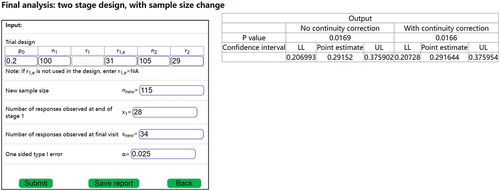
In Figure 4, $p_0=0.2$, $n_1=100$, $r_{1,\mathit{e}}=31$, $n_2=105$, $r_2=29$. The number of observed responses at the interim analysis (at $n_1$) is $x_1=28$. The value of $r_1$ is not needed for the final analysis, because the trial continued after the interim analysis, and thus the final analysis does not need the value of $r_1$ (only $r_{1,\mathit{e}}$ is needed). After the interim analysis, the sample size was changed to $n_{\mathit{new}}=115$. The final observed number of responses is $x_{\mathit{new}}=34$. We note that the final analysis only involves $x_{\mathit{new}}$, but not the adjusted $r_{\mathit{new}}$ or $r_{new}^{cor}$. Assuming that simulations had been conducted at the trial design stage (e.g. Figures 2 and 3) to determine whether continuity correction is necessary. If continuity correction was not necessary, then the output without continuity will be used as the final inference, with the estimated response rate of $\hat{p}=0.29152$, the 95% confidence interval of (0.206993, 0.375902), and a p-value of 0.0169. Otherwise, using inference with continuity correction, the estimated response rate of $\hat{p}=0.291644$, the 95% confidence interval of (0.206728, 0.375954), and a p-value of 0.0166.

4. Design examples and simulations

4.1. Design examples

Suppose that a single-arm phase II trial is being designed. Suppose that $p_0=0.2$, $p_{\mathit{low}}=0.33$, $p_1=0.4$. There are several possible designs: i) $\mathit{S}\left(p_0,p_{\mathit{low}},\mathit{\alpha },\mathit{\beta }\right)$: Simon’s design with $p_1=p_{\mathit{low}}=0.33$; ii) $\mathit{S}\left(p_0,p_1,\mathit{\alpha },\mathit{\beta }\right)$: Simon’s design with $p_1=0.4$; iii) The hybrid design and the midpoint design ($\mathit{\rho }$ = 0.5) with $p_{\mathit{low}}=0.33$, $p_1=0.4$. Minimum value for $\mathrm{\Delta }{n}_{12}$ is set to be 5 for purpose of discussion. iv) the three-stage design. $\left({\alpha }_1,{\alpha }_2\right)=\left(0.001,0.024\right)$ is used for discussion. Investigators can use any $\left({\alpha }_1,{\alpha }_2\right)$, as long as ${\alpha }_1+{\alpha }_2\le \mathit{\alpha }$. Note that the search for $r_{1,\mathit{e}}$ and $r_{2,\mathit{e}}$ is such that ${\alpha }_1,{\alpha }_2$ are associated with $r_{1,\mathit{e}}$ and $r_{2,\mathit{e}}$ as actual probabilities of $\mathit{\alpha }$-spending, not nominal $\mathit{\alpha }$-spending (the sum of nominal $\mathit{\alpha }$-spending will be greater than $\mathit{\alpha }$). So the condition of ${\alpha }_1+{\alpha }_2\le \mathit{\alpha }$ is not a conservative requirement. In practice, larger ${\alpha }_1$ may be selected if the investigators believe (e.g., based on literature and/or clinical evidence) that the response rate is more likely to be closer to $p_1$, smaller ${\alpha }_1$ may be selected otherwise. The impact of the $\mathit{\alpha }$-spending can be investigated with simulations (with SSR) to optimize power for the interested range of the response rate, $\left(p_{\mathit{low}},p_1\right)$. Tables 3 and 4 present design examples. $\mathit{err}$ indicates type I error, and PW denotes power.

Table 3. Simon’s two-stage design with augmentation (fixed sample).

$\mathit{S}\left(p_0,p_{\mathit{low}},\mathit{\alpha },\mathit{\beta }\right)$
	$r_1$	$n_1$	$r_2$	$n_2$	$\mathit{err}$	$\mathit{EN}\left(p_0\right)$	$\mathit{PET}\left(p_{\mathit{low}}\right)$	$\mathit{PW}\left(p_1\right)$	$\mathit{PW}\left(p_{\mathit{low}}\right)$
minimax	25	100	32	119	0.0248	101.7	0.053	0.900	0.900
optimal	11	50	36	137	0.0244	75.2	0.063	0.902	0.902
Average	18	75	34	128	0.0238	83.3	0.060	0.900	0.900
$\mathit{S}\left(p_0,p_1,\mathit{\alpha },\mathit{\beta }\right)$
minimax	9	37	16	53	0.0248	40.1	0.172	0.900	0.596
optimal	5	22	19	66	0.0242	33.8	0.216	0.904	0.632
Average	7	30	17	57	0.0236	36.5	0.176	0.900	0.607

Table 4. The expanded designs (fixed sample).

	$r_{1,\mathit{f}}$		$n_1$	$r_{1,\mathit{e}}$	$r_2$	$n_2$	$\mathit{err}$	$\mathit{EN}\left(p_0\right)$	$\mathit{PET}\left(p_{\mathit{low}}\right)$		$\mathit{PW}\left(p_1\right)$	$\mathit{PW}\left(p_{\mathit{low}}\right)$
Two-stage: The hybrid design: $\mathit{min}\text{(}\mathit{\Delta }{n}_{12}\text{)}=5$, $\left({\alpha }_1,{\alpha }_2\right)=\left(0.001,0.024\right)$
Stage 1 minimax	25		100	33	29	105	0.0223	100.4	0.053		0.994	0.858
Stage 1 optimal	11		50	NA	17	56	0.0219	51.7	0.063		0.911	0.604
Stage 1 Average	18		75	26	23	80	0.0217	75.8	0.060		0.976	0.752
Two-stage: The midpoint design: $\mathit{\rho }=0.5$. $\mathit{min}\left(\mathrm{\Delta }{n}_{12}\right)=5$, $\left({\alpha }_1,{\alpha }_2\right)=\left(0.001,\mathrm{.0.024}\right)$
Stage 1 minimax	17		69	25	22	74	0.0159	69.7	0.086		0.956	0.678
Stage 1 optimal	7		36	NA	17	56	0.0218	44.7	0.056		0.910	0.602
Stage 1 Average	12		53	NA	18	59	0.0185	54.5	0.069		0.914	0.600
	$r_{1,\mathit{f}}$	$n_1$	$r_2$	$r_{2,\mathit{e}}$	$n_2$	$r_3$	$n_3$	$\mathit{err}$	$\mathit{EN}\left(p_0\right)$	$\mathit{PET}\left(p_{\mathit{low}}\right)$	$\mathit{PW}\left(p_1\right)$	$\mathit{PW}\left(p_{\mathit{low}}\right)$
The three-stage design. $\mathit{min}\left(\mathrm{\Delta }{n}_{23}\right)=5$ , $\left({\alpha }_1,{\alpha }_2,{\alpha }_3\right)=\left(0,0.001,\mathrm{.0.024}\right)$
Stage 1 minimax	8	37	22	33	100	29	105	0.019	57.5	0.098	0.981	0.810
Stage 1 optimal	3	22	11	NA	50	17	56	0.022	42.3	0.084	0.908	0.600
Stage 1 Average	6	30	16	26	75	23	80	0.020	48.5	0.097	0.963	0.724

4.2. Simulations

If the true response rate is $p_{\mathit{low}}=0.33$, then both the Simon’s design $\mathit{S}\left(p_0,p_1,\mathit{\alpha },\mathit{\beta }\right)$, with $p_1=0.4$, and all of the expanded designs with $p_1=0.4$, and $p_{\mathit{low}}=0.33$, will have power less than $1-\mathit{\beta }$. We conducted the simulations to check if combining with SSR can improve the power to be close to $1-\mathit{\beta }$ for each of the designs. We use a hypothetical maximum sample size of 140. This is close to $n_2^{Si\mathrm{mon}:opt}\left(p_0,p_{\mathit{low}}\right)=137$. The critical boundaries without continuity correction are used when the type I error is adequately controlled without the correction. Otherwise, the critical boundaries with continuity correction are used.

Simulations were conducted to investigate the operating characteristics of each design with SSR and the results are presented in Tables 4–6. The algorithm for the SSR is described in section 3.1.1. The results include: type I error ($p_0=0.2$) with and without continuity correction ($\mathit{er}{r}_{\mathit{CC}}$ and $\mathit{err}$), power under $p_{\mathit{low}}=0.33$ and $p_1=0.4$, with or without continuity correction ($\mathit{P}{W}_{\mathit{CC}}$ and $\mathit{PW}$), expected sample size under both $p_0$ and $p_{\mathit{low}}$ ($\mathit{EN}\left(p_0\right)$ and $\mathit{EN}\left(p_{\mathit{low}}\right)$, as well as the probability of early termination under $p_{\mathit{low}}$ ($\mathit{PET}\left(p_{\mathit{low}}\right)$. All the simulations are supported by the DACT software. DACT provides all the outputs summarized in Tables 4–6.

Table 5. Simulation on SSR with Simon’s two-stage design.

Design: The original Simon’s design $\mathit{S}\left(p_0,p_1,\mathit{\alpha },\mathit{\beta }\right)$ with $p_1=0.4$; Simulations: $\mathit{p}=p_{\mathit{low}}=0.33$
Fixed sample $\mathit{S}\left(p_0,p_1,\mathit{\alpha },\mathit{\beta }\right)$design					With SSR
	$r_1$	$n_1$	$r_2$	$n_2$	$\mathit{EN}\left(p_0\right)$	$\mathit{err}$	$\mathit{er}{r}_{\mathit{CC}}$	PET$\left(p_{\mathit{low}}\right)$	$\mathit{EN}\left(p_{\mathit{low}}\right)$	$\mathit{PW}\left(p_{\mathit{low}}\right)$	$\mathit{P}{W}_{\mathit{CC}}\left(p_{\mathit{low}}\right)$
minimax	9	37	16	53	50.7	0.0245^1	0.0201	0.171	66.5	0.727^1	0.691
optimal	5	22	19	66	42.7	0.0213^1	0.021	0.213	65.4	0.668^1	0.634
Average	7	30	17	57	48.1	0.0248^1	0.0211	0.177	66.5	0.682^1	0.662

^aContinuity corrected critical boundaries unnecessary; ²Continuity corrected critical boundaries necessary.

Table 6. Simulation SSR with the expanded two-stage designs.

Fixed sample hybrid design						With SSR
	$r_{1,\mathit{f}}$	$n_1$	$r_{1,\mathit{e}}$	$r_2$	$n_2$	$\mathit{err}$	$\mathit{er}{r}_{\mathit{CC}}$	$\mathit{EN}\left(p_0\right)$	PET$\left(p_{\mathit{low}}\right)$	$\mathit{EN}\left(p_{\mathit{low}}\right)$	$\mathit{PW}\left(p_{\mathit{low}}\right)$	$\mathit{P}{W}_{\mathit{CC}}\left(p_{\mathit{low}}\right)$
Two-stage: The hybrid design: $\mathit{min}\left(\mathrm{\Delta }{n}_{12}\right)=5$
Stage 1 minimax	25	100	33	29	105	0.0259	0.0235^2	102.3	0.054	107.3	0.90	0.881^2
Stage 1 optimal	11	50	NA	17	56	0.0273	0.0243^2	72.3	0.064	80.5	0.789	0.735^2
Stage 1 Average	18	75	26	23	80	0.0261	0.0224^2	83.1	0.062	91	0.862	0.816^2
Stage 1 minimax	17	69	25	22	74	0.0194^1	0.0173	76.7	0.086	87.7	0.807^1	0.763
Stage 1 optimal	7	36	NA	17	56	0.0234^1	0.0198	75	0.055	80.6	0.774^1	0.740
Stage 1 Average	12	53	NA	18	59	0.0223^1	0.0196	71.9	0.068	82.7	0.787^1	0.720

^aContinuity corrected critical boundaries unnecessary; ²Continuity corrected critical boundaries necessary.

All type I errors without continuity correction ($\mathit{err}$) were less than 0.025. Hence, continuity correction was not necessary for the scenarios in Table 4.

All type I error without continuity correction ($\mathit{err}$) for the hybrid design exceeded 0.025, while the continuity corrected type I error ($\mathit{er}{r}_{\mathit{CC}})$ were less than 0.025. Hence, continuity correction was necessary for hybrid design the scenarios in Table 5.

All type I error without continuity ($\mathit{err}$) for the midpoint design were less than 0.025. Hence, continuity correction was not necessary for the hybrid design in the scenarios in Table 5.

The type I error without continuity correction ($\mathit{err}$) for the optimal design exceeded 0.025, while the continuity corrected type I error ($\mathit{er}{r}_{\mathit{CC}})$ for the optimal were less than 0.025. Hence, continuity correction was necessary for optimal design in the scenarios in Table 6.

The type I error without continuity correction ($\mathit{err}$) for the minimax and average designs were less than 0.025. Hence, continuity correction was not necessary for the minimax and average designs in the scenarios in Table 6. Tables 5, 6 and 7 show that the three-stage design has the smallest $\mathit{EN}\left(p_0\right)$.

Table 7. Simulation SSR with the expanded three-stage designs.

Fixed sample three-stage design								With SSR
	$r_{1,\mathit{f}}$	$n_1$	$r_2$	$r_{2,\mathit{e}}$	$n_2$	$r_3$	$n_3$	$\mathit{err}$	$\mathit{er}{r}_{\mathit{CC}}$	$\mathit{EN}\left(p_0\right)$	PET$\left(p_{\mathit{low}}\right)$	$\mathit{EN}\left(p_{\mathit{low}}\right)$	$\mathit{PW}\left(p_{\mathit{low}}\right)$	$\mathit{P}{W}_{\mathit{CC}}\left(p_{\mathit{low}}\right)$
The three-stage design. $\mathit{min}\left(\mathrm{\Delta }{n}_{23}\right)=5$
Stage 1 minimax	8	37	22	33	100	29	105	0.0223^1	0.0193	63.8	0.098	102	0.850^1	0.834
Stage 1 optimal	3	22	11	NA	50	17	56	0.0272	0.0233^2	63.3	0.084	80	0.786	0.736^2
Stage 1 Average	6	30	16	26	75	23	80	0.0247^1	0.0207	62.3	0.098	87.4	0.819^1	0.784

^aContinuity corrected critical boundaries unnecessary; ²Continuity corrected critical boundaries necessary.

If the true response rate is $\mathit{p}=p_{\mathit{low}}=0.33$,

• The power of $\mathit{S}\left(p_0,p_1,\mathit{\alpha },\mathit{\beta }\right)$+SSR (Table 4) under $\mathit{p}=p_{\mathit{low}}$were only 0.727 for the optimal design, and even smaller for the minimax design + SSR at 0.668. Confirming that simply adding SSR to $\mathit{S}\left(p_0,p_1,\mathit{\alpha },\mathit{\beta }\right)$ could be insufficient to provide desirable power for all $\mathit{p}$ between $p_{\mathit{low}}$ and $p_1$. Larger sample sizes $n_1$ and $n_2$ would be necessary to achieve larger power.

• The purpose for introducing the expansions was that the expansions in combination with SSR will have more power than $\mathit{S}\left(p_0,p_1,\mathit{\alpha },\mathit{\beta }\right)$ combined with SSR. It is noted that: i) The sample sizes ($n_1$ and $n_2$) for all the expanded designs were larger than that for $\mathit{S}\left(p_0,p_1,\mathit{\alpha },\mathit{\beta }\right)$ and were permissible. Interim analysis with larger sample sizes (at $n_1)$have more information time and smaller variation, and the interim analysis results are more accurate. Hence, the SSR with the expanded designs were more reliable than the SSR with $\mathit{S}\left(p_0,p_1,\mathit{\alpha },\mathit{\beta }\right)$.

• Although the sample size of the three-stage designs was larger than that of $\mathit{S}\left(p_0,p_1,\mathit{\alpha },\mathit{\beta }\right)$, the simulated $\mathit{EN}\left(p_0\right)$ for the three-stage design combined with SSR (Table 6) were very close to that of $\mathit{S}\left(p_0,p_1,\mathit{\alpha },\mathit{\beta }\right)$ combined with SSR (Table 4). i.e., the three-stage design combined with SSR performs well with Simon’s considerations.

• $\mathit{PET}\left(p_{\mathit{low}}\right)>0.17>\mathit{\beta }$ for Simon’s design $\mathit{S}\left(p_0,p_1,\mathit{\alpha },\mathit{\beta }\right)$, while $\mathit{PET}\left(p_{\mathit{low}}\right)<\mathit{\beta }$ for all the expanded designs.

• The simulated power does not exceed $1-\mathit{PET}\left(p_{\mathit{low}}\right)$ for all designs.

5. Discussions

Lin and Shih (2004) facilitate hypothesis tests for two possible response rates, an optimistic and a skeptical target rate. From this perspective, Lin and Shih (2004) is more flexible than either Simon’s design Simon (1989) or that of Jung et al. (2004), since both of them conducts hypothesis testing on only one target response rate. However, in general, SSR (either conditional error function based, such as that by Englert and Kieser (2012); Englert and S (2013); or adaptive sequential methods in our proposal) allows for a range of possible response rates and is thus more flexible than Lin and Shih (2004).

Simon’s designs only use a binomial endpoint, which may be considered to be a limitation. However, a response rate (such as ORR) may be more intuitive than other endpoints. Such intuitiveness may be the reason for the popularity of Simon’s design. On the other hand, expanding Simon’s design using other endpoints (e.g., progression-free survival) could offer more options for trial investigators conducting phase II oncology trials. However, that is beyond the scope of this article.

We propose several expansions for Simon’s design. They are intended to be used together with SSR, such that the planned sample size is sufficient to provide power for when the response rate is $p_1$, and with the flexibility to increase sample size if the observed response rate is closer to $p_{\mathit{low}}$. The simulations show that all of expanded design combined with SSR have more desirable power than Simon’s design combined with SSR, as intended. The three-stage design is statistically more efficient than the two-stage expansions because it has similar simulated power but a smaller $\mathit{EN}\left(p_0\right)$ than the other expansions. Three-stage design has been previously proposed (Chen 1997; Ensign et al. 1994). It is recognized that a three-stage design is operationally more complicated than a two-stage design. We note that most clinical trials involve at most one interim analysis. However, when feasible, statistical optimality could be preferable despite the added operational complexity. For example, some single-arm phase II oncology trials do conduct multiple interim analysis (e.g., the Zuma-1 trial protocol (2015a); Zuma-2 trial protocol (2015b)) . If a three-stage design is not feasible, either the hybrid or the midpoint design may be used.

In practice, the operating characteristics of any of the proposed designs can be influenced by several factors, such as $p_0,p_1$, $p_{\mathit{low}}$ $p_{\mathit{high}}$, $N_{\mathit{max}}$., $\mathit{min}\left(\mathrm{\Delta }{n}_{12}\right)$ and $\left({\alpha }_1,{\alpha }_2\right)$ (for two-stage expanded designs), $\mathit{min}\left(\mathrm{\Delta }{n}_{23}\right)$ and $\left({\alpha }_1,{\alpha }_2,{\alpha }_3\right)$ (for three-stage expanded designs). For the midpoint design, the OCs are also affected by the choices of $\mathit{\rho }$. The OCs of each design under consideration should be thoroughly investigated with simulations. Designs that optimize the considerations of budget, patient enrollment, and feasibility can then be selected. All these simulations can be conducted with the DACT software. In general, we recommend the three-stage design because of its statistical efficiency.

Disclosure statement

No potential conflict of interest was reported by the author(s).

Supplemental data

Supplemental data for this article can be accessed online at https://doi.org/10.1080/10543406.2024.2341673.

Additional information

Funding

The author(s) reported there is no funding associated with the work featured in this article.

References

- Bauer, P., and K. Kohne. 1994. Evaluation of experiments with adaptive interim analyses. Biometrics Bulletin 50 (4):1029–1041. doi:10.2307/2533441.
- Chang, M. N., T. M. Therneau, H. S. Wieand, and S. S. Cha. 1987, Dec. Designs for group sequential phase II clinical trials. Biometrics Bulletin 43(4):865–874. doi:10.2307/2531540.
- Chen, T. T. 1997, Dec 15. Optimal three-stage designs for phase II cancer clinical trials. Statistics in Medicine 16 (23):2701–2711. doi:10.1002/(sici)1097-0258(19971215)16:23<2701:aid-sim704>3.0.co;2-1. PMID: 9421870.
- Chen, Y. H. J., D. L. DeMets, and K. K. G. Lan. 2004 Apr 15. Increasing the sample size when the unblinded interim result is promising. Statistics in Medicine 23(7):1023–1038. doi:10.1002/sim.1688.
- Cui, L., H. M. Hung, and S. J. Wang. 1999. Modification of sample size in group sequential clinical trials. Biometrics Bulletin 55 (3):853–857. doi:10.1111/j.0006-341X.1999.00853.x.
- Devore, J. L. 1995. Probability and statistics for engineering and the sciences. 4th ed. USA: Duxbury Press.
- Englert, S., and M. Kieser. 2012, September. Improving the flexibility and efficiency of phase II designs for oncology trials. Biometrics Bulletin 68(3):886–892. doi:10.1111/j.1541-0420.2011.01720.x.
- Englert, S., and M. K. S. 2013, Nov. Optimal adaptive two-stage designs for phase II cancer clinical trials. Biometrical Journal 55(6):955–968. doi:10.1002/bimj.201200220.
- Ensign, L. G., E. A. Gehan, D. S. Kamen, and P. F. Thall. 1994 Sep 15. An optimal three-stage design for phase II clinical trials. Statistics in Medicine 13(17):1727–1736. doi:10.1002/sim.4780131704.
- Feller, W. 1945. On the normal approximation to the binomial distribution. The Annals of Mathematical Statistics 16 (4):319–329. doi:10.1214/aoms/1177731058.
- Gao, P., L. Liu, and C. Mehta. 2013 Oct 15. Exact inference for adaptive group sequential designs. Statistics in Medicine 32(23):3991–4005. doi:10.1002/sim.5847.
- Gao, P., J. H. Ware, and C. Mehta. 2008. Sample size re-estimation for adaptive sequential designs. Journal of Biopharmaceutical Statistics 18 (6):1184–1196. doi:10.1080/10543400802369053.
- Jennison, C., and B. Turnbull. 2003. Mid-course sample size modification in clinical trials based on the observed treatment effect. Statistics in Medicine 22 (6):971–993. doi:10.1002/sim.1457.
- Jennison, C., and B. Turnbull. 2006, Mar. Adaptive and non-adaptive group sequential tests. Biometrika 93(1):1–21. doi:10.1093/biomet/93.1.1.
- Jung, S.-H., T. Lee, K. M. Kim, and S. L. George. 2004. Admissible two-stage designs for phase II cancer clinical trials. Statistics in Medicine 23 (4):561–569. doi:10.1002/sim.1600.
- Kunzmann, K., and M. Kieser. 2016. Optimal adaptive two-stage designs for single-arm trial with binary endpoint. arXiv:1605.00249 [stat.AP].
- Lan, K. K. G., and D. L. DeMets. 1983. Discrete sequential boundaries for clinical trials. Biometrika 70 (3):659–663. doi:10.2307/2336502.
- Lin, Y., and W. J. Shih. 2004, Jun. Adaptive two-stage designs for arm phase Ha cancer clinical trials. Biometrics Bulletin 60(2):482–490. doi:10.1111/j.0006-341X.2004.00193.x.
- Müller, H. H., and H. Schäfer. 2001. Adaptive group sequential designs for clinical trials: Combining the advantages of adaptive and of classical group sequential approaches. Biometrics. 57 (3):886–91.
- O’Brien, P. C., and T. R. Fleming. 1979. A multiple testing procedure for clinical trials. Biometrics Bulletin 35 (3):549–556. doi:10.2307/2530245.
- Pocock, S. J. 1977. Group sequential methods in the design and analysis of clinical trials. Biometrika 64 (2):191–199. doi:10.1093/biomet/64.2.191.
- Proschan, M. A., and S. A. Hunsberger. 1995, Dec. Designed extension of studies based on conditional power. Biometrics Bulletin 51(4):1315–1324. doi:10.2307/2533262.
- Simon, R. 1989. Optimal two-stage designs for phase II clinical trials. Controlled Clinical Trials 10 (1):1–10. doi:10.1016/0197-2456(89)90015-9.
- U.S. Food and Drug Administration. 2018, Dec. Oncology center of excellence/center for drug evaluation and research (CDER)/center for biologics evaluation and research (CBER). Clinical trial endpoints for the approval of cancer drugs and biologics. guidance for industry.
- U.S. Food and Drug Administration (CDER and CBER). 2019. Guidance for industry adaptive design clinical trials for drugs and biologics.
- Zuma-1 trial protocol, 2015. https://www.nejm.org/doi/suppl/10.1056/NEJMoa1707447/suppl_file/nejmoa1707447_protocol.pdf.
- Zuma-2 trial protocol, 2015. https://www.nejm.org/doi/suppl/10.1056/NEJMoa1914347/suppl_file/nejmoa1914347_protocol.pdf.