Group Selection and Shrinkage: Structured Sparsity for Semiparametric Additive Models

Abstract

Sparse regression and classification estimators that respect group structures have application to an assortment of statistical and machine learning problems, from multitask learning to sparse additive modeling to hierarchical selection. This work introduces structured sparse estimators that combine group subset selection with shrinkage. To accommodate sophisticated structures, our estimators allow for arbitrary overlap between groups. We develop an optimization framework for fitting the nonconvex regularization surface and present finite-sample error bounds for estimation of the regression function. As an application requiring structure, we study sparse semiparametric additive modeling, a procedure that allows the effect of each predictor to be zero, linear, or nonlinear. For this task, the new estimators improve across several metrics on synthetic data compared to alternatives. Finally, we demonstrate their efficacy in modeling supermarket foot traffic and economic recessions using many predictors. These demonstrations suggest sparse semiparametric additive models, fit using the new estimators, are an excellent compromise between fully linear and fully nonparametric alternatives. All of our algorithms are made available in the scalable implementation grpsel. Supplementary materials for this article are available online.

Keywords:

• Group lasso
• Group sparsity
• Group subset selection
• Structured sparsity
• Variable selection

1 Introduction

Sparsity over group¹ structures arises in connection with a myriad of statistical and machine learning problems, for example, multitask learning (Obozinski, Taskar, and Jordan 2006), sparse additive modeling (Ravikumar et al. 2009), and hierarchical selection (Lim and Hastie 2015). Even sparse linear modeling can involve structured sparsity, such as when a categorical predictor is represented as a sequence of dummy variables. In certain domains, groups may emerge naturally, for example, disaggregates of the same macroeconomic series or genes of the same biological path. The prevalence of such problems motivates principled estimation procedures capable of encoding structure into the fitted models they produce.

Given response $\mathbf{y}={(y_1,\dots ,y_n)}^{\mathrm{\top }}\in {ℝ}^n$, predictors $\mathbf{X}={({\mathbf{x}}_1,\dots ,{\mathbf{x}}_n)}^{\mathrm{\top }}\in {ℝ}^{n\times p}$, and nonoverlapping groups ${\mathcal{G}}_1,\dots ,{\mathcal{G}}_g\subseteq \{1,\dots ,p\}$, group lasso (Yuan and Lin 2006; Meier, van de Geer, and Bühlmann 2008) solves $$\underset{\mathit{\beta }\in {ℝ}^p}{\min }\sum _i\ell \left({\mathbf{x}}_i^{\mathrm{\top }}\mathit{\beta },y_i\right)+\sum _k{\lambda }_k\Vert {\mathit{\beta }}_k\Vert ,$$ where $\ell :{ℝ}^2\to {ℝ}_{+}$ is a loss function (e.g., square loss for regression or logistic loss for classification), ${\lambda }_1,\dots ,{\lambda }_g$ are nonnegative tuning parameters, and ${\mathit{\beta }}_k\in {ℝ}^{p_k}$ are the coefficients $\mathit{\beta }$ indexed by ${\mathcal{G}}_k$. Group lasso couples coefficients via their l₂-norm so that all predictors in a group are selected together.

Just as lasso (Tibshirani 1996) is the continuous relaxation of the combinatorially hard problem of best subset selection (“best subset”), so is group lasso the relaxation of the combinatorial problem of group subset selection (“group subset”): $$\underset{\mathit{\beta }\in {ℝ}^p}{\min }\sum _i\ell \left({\mathbf{x}}_i^{\mathrm{\top }}\mathit{\beta },y_i\right)+\sum _k{\lambda }_{k}1(\Vert {\mathit{\beta }}_k\Vert \ne 0).$$

Unlike group lasso, which promotes group sparsity implicitly by nondifferentiability of the l₂-norm at the null vector, group subset explicitly penalizes the number of nonzero groups. Consequently, one might interpret group lasso as a compromise made in the interest of computation. However, group lasso has a trick up its sleeve that group subset does not: shrinkage. Shrinkage estimators such as lasso are more robust than best subset to noise (Breiman 1996; Hastie, Tibshirani, and Tibshirani 2020). This consideration motivates one to shrink the group subset estimator: (1.1) $$\underset{\mathit{\beta }\in {ℝ}^p}{\min }\sum _i\ell \left({\mathbf{x}}_i^{\mathrm{\top }}\mathit{\beta },y_i\right)+\sum _k{\lambda }_{0k}1(\Vert {\mathit{\beta }}_k\Vert \ne 0)+\sum _k{\lambda }_{1k}\Vert {\mathit{\beta }}_k\Vert .$$(1.1)

In contrast to group lasso and group subset, (1.1) directly controls both group sparsity and shrinkage via separate penalties—selection via group subset and shrinkage via group lasso. The combination of best subset and lasso in the unstructured setting results in good predictive models with low false positive selection rates (Mazumder, Radchenko, and Dedieu 2023).

Unfortunately, the estimators (1.1), including group lasso and group subset as special cases, do not accommodate overlap among groups. Specifically, if two groups overlap, one cannot be selected independently of the other. To encode sophisticated structures, such as hierarchies or graphs, groups must often overlap. To address this issue, one can introduce group-specific vectors ${\overline{\mathit{\nu }}}_k\in {ℝ}^p(k=1,\dots ,g)$ that are zero everywhere except at the positions indexed by ${\mathcal{G}}_k$. Letting $\mathcal{V}$ be the set of all tuples $\overline{\mathit{\nu }}:=({\overline{\mathit{\nu }}}_1,\dots ,{\overline{\mathit{\nu }}}_g)$ with elements satisfying this property, group subset with shrinkage becomes (1.2) $$\underset{\stackrel{\mathit{\beta }\in {ℝ}^p,\overline{\mathit{\nu }}\in \mathcal{V}}{\mathit{\beta }=\sum _k{\overline{\mathit{\nu }}}_k}}{\min }\sum _i\ell \left({\mathbf{x}}_i^{\mathrm{\top }}\mathit{\beta },y_i\right)+\sum _k{\lambda }_{0k}1(\Vert {\overline{\mathit{\nu }}}_k\Vert \ne 0)+\sum _k{\lambda }_{1k}\Vert {\overline{\mathit{\nu }}}_k\Vert .$$(1.2)

The vectors ${\overline{\mathit{\nu }}}_1,\dots ,{\overline{\mathit{\nu }}}_g$ are a decomposition of $\mathit{\beta }$ into a sum of latent coefficients that facilitate selection of overlapping groups. For instance, if three predictors, x₁, x₂, and x₃, are spread across two groups, ${\mathcal{G}}_1=\{1,2\}$ and ${\mathcal{G}}_2=\{2,3\}$, then ${\beta }_1={\overline{\nu }}_{1,1}$, ${\beta }_2={\overline{\nu }}_{2,1}+{\overline{\nu }}_{2,2}$, and ${\beta }_3={\overline{\nu }}_{3,2}$. Since β₂ has a separate latent coefficient for each group, ${\mathcal{G}}_1$ or ${\mathcal{G}}_2$ can be selected independently of the other. This latent coefficient approach originated for group lasso with Jacob, Obozinski, and Vert (2009) and Obozinski, Jacob, and Vert (2011). When all groups are disjoint, (1.2) reduces exactly to (1.1).

This article develops computational methods and statistical theory for group subset with and without shrinkage. Via the formulation (1.2), our work accommodates the general overlapping groups setting. On the computational side, we develop algorithms that scale to compute quality (approximate) solutions of the combinatorial optimization problem. Our framework comprises coordinate descent and local search and applies to general smooth convex loss functions (i.e., regression and classification), building on recent advances for best subset (Hazimeh and Mazumder 2020; Dedieu, Hazimeh, and Mazumder 2021). In contrast to existing computational methods for group subset (Guo, Berman, and Gao 2014; Bertsimas and King 2016), which rely on branch-and-bound or commercial mixed-integer optimizers, our methods scale to instances with millions of predictors or groups. We implement our framework in the publicly available R package grpsel. On the statistical side, we establish new error bounds for group subset with and without shrinkage. The bounds apply in the overlapping setting and allow for model misspecification. The analysis sheds light on the advantages of structured sparsity and the benefits of shrinkage.

The new estimators have application to a broad range of statistical problems. We focus on sparse semiparametric additive modeling (Chouldechova and Hastie 2015; Lou 2016), a procedure that models y as a sum of univariate functions f_j : $$g(\mathrm{E}[y])=\sum _j{f}_j(x_j),$$ where g is a given link function (e.g., identity for regression or logit for classification). The appeal of this model is its flexibility. An individual f_j can be a complex nonlinear function, a simple linear function $f_j(x_j)={\beta }_j{x}_j$, or a zero function $f_j(x_j)=0$, the latter implying no effect of x_j . Chouldechova and Hastie (2015) estimate these models using group lasso with overlapping groups and regression splines. Briefly summarized, this approach takes $f_j(x_j)={\sum }_{l=1}^m{\beta }_{jl}{b}_l(x_j)$, where $b_l(x_j)$ are the basis functions of an m-term regression spline in which $b_1(x_j)=x_j$. Two groups are created for each x_j : a linear group containing the linear term $b_1(x_j)$, and a nonlinear group containing all $b_1(x_j),\dots ,b_m(x_j)$. Group lasso is then applied to these overlapping groups. If the jth nonlinear group is selected, f_j is fit as a nonlinear function, regardless of whether the jth linear group is also selected (if it is, the fit is still nonlinear and the two coefficients on $b_1(x_j)$ are added together). If only the linear group is selected, the fit is linear. If neither group is selected, x_j is excluded from the model.

After conducting synthetic experiments on the efficacy of our estimators in fitting sparse semiparametric additive models (“semiparametric models”) using the above approach, we carry out two empirical studies. The first study involves modeling supermarket foot traffic using sales volumes on different products. Only a fraction of supermarket products are traded in volume, necessitating sparsity. The second study involves modeling recessionary periods in the economy using macroeconomic series. The macroeconomic literature contains many examples of sparse linear modeling (De Mol, Giannone, and Reichlin 2008; Li and Chen 2014), yet theory does not dictate linearity. Together these studies suggest sparse semiparametric models are an excellent compromise between fully linear and fully nonparametric alternatives.

Independently and concurrently to this work, Hazimeh, Mazumder, and Radchenko (2023) study computation and theory for group subset with nonoverlapping groups. Their algorithms likewise build on Hazimeh and Mazumder (2020) but apply only to square loss regression. Also related is Zhang et al. (2023) who propose a computational “splicing” technique for group subset that appears promising, though they do not consider overlapping groups or shrinkage.

1.1 Organization

The article is structured as follows. Section 2 presents computational methods. Section 3 provides statistical theory. Section 4 discusses the R implementation. Section 5 describes simulation experiments. Section 6 reports data analyses. Section 7 closes the article.

2 Computation

This section introduces our optimization framework and its key components: coordinate descent and local search. The framework applies to any smooth loss function $\ell (z,y)$ convex in z. The discussion below addresses the specific cases of square loss $\ell (z,y)={(y-z)}^2/2$, which is suitable for regression, and logistic loss $\ell (z,y)=-y\hspace{0.17em}\log \hspace{0.17em}(z)-(1-y)\hspace{0.17em}\log \hspace{0.17em}(1-z)$, which is suitable for classification. Throughout this section, the predictor matrix X is assumed to have columns with mean zero and unit l₂-norm.

2.1 Problem Reformulation

From a computational perspective, it helps to reformulate the group subset problem (1.2) as an unconstrained minimization problem involving only the latent coefficients $\overline{\mathit{\nu }}$. For this task, we denote by ${\mathit{\nu }}_k\in {ℝ}^{p_k}$ the restriction of ${\overline{\mathit{\nu }}}_k$ to the coordinates indexed by group k. No information is lost in this restriction since all elements not indexed by ${\mathcal{G}}_k$ are zero. We also introduce the vector $\mathit{\nu }:={({\mathit{\nu }}_1^{\mathrm{\top }},\dots ,{\mathit{\nu }}_g^{\mathrm{\top }})}^{\mathrm{\top }}\in {ℝ}^{\sum _k{p}_k}$ formed by vertically concatenating the vectors ${\mathit{\nu }}_1,\dots ,{\mathit{\nu }}_g$. Consider now the unconstrained minimization problem $$\underset{\mathit{\nu }\in {ℝ}^{\sum _k{p}_k}}{\min }F(\mathit{\nu }):=L(\mathit{\nu })+R(\mathit{\nu }).$$

Here, the function $L(\mathit{\nu })$ is the loss term: $$L(\mathit{\nu }):=\sum _i\ell \left(\sum _k{\mathbf{x}}_{ik}^{\mathrm{\top }}{\mathit{\nu }}_k,y_i\right),$$ where ${\mathbf{x}}_{ik}$ is the ith row of the matrix ${\mathbf{X}}_k$, with ${\mathbf{X}}_k$ the restriction of X to the columns indexed by group k. The function $R(\mathit{\nu })$ is the regularizer term: $$R(\mathit{\nu }):=\sum _k\left({\lambda }_{0k}1(\Vert {\mathit{\nu }}_k\Vert \ne 0)+{\lambda }_{1k}\Vert {\mathit{\nu }}_k\Vert \right).$$

Observe that the loss $L(\mathit{\nu })$ is exactly equivalent to that in (1.2) since $$\sum _i\ell \left(\mathrm{}\sum _k{\mathbf{x}}_{ik}^{\mathrm{\top }}{\mathit{\nu }}_k,y_i\mathrm{}\right)=\sum _i\ell \left(\mathrm{}{\mathbf{x}}_i^{\mathrm{\top }}\sum _k{\overline{\mathit{\nu }}}_k,y_i\mathrm{}\right)=\sum _i\ell \left(\mathrm{}{\mathbf{x}}_i^{\mathrm{\top }}\mathit{\beta },y_i\mathrm{}\right).$$

The regularizer $R(\mathit{\nu })$ is likewise equivalent because $\Vert {\mathit{\nu }}_k\Vert =\Vert {\overline{\mathit{\nu }}}_k\Vert$. As the equalities immediately above suggest, it is straightforward to recover $\mathit{\beta }$ from $\mathit{\nu }$.

We refer to the group support, or active set of groups, of the vector $\mathit{\nu }$ as the set of nonzero group indices: $$\text{gs}(\mathit{\nu }):=\{k\in \{1,\dots ,g\}:\Vert {\mathit{\nu }}_k\Vert \ne 0\}.$$

The complement of the active set is referred to as the inactive set.

2.2 Coordinate Descent

Coordinate descent algorithms are optimization routines that minimize along successive coordinate hyperplanes. The coordinate descent scheme developed here iteratively fixes all but one group of coordinates (a coordinate group) and minimizes in the directions of these coordinates.

The objective function $F(\mathit{\nu })$ is a sum of smooth convex and discontinuous nonconvex functions and is hence discontinuous nonconvex. The minimization problem with respect to group k is (2.1) $$\underset{\mathit{\xi }\in {ℝ}^{p_k}}{\min }F({\mathit{\nu }}_1,\dots ,{\mathit{\nu }}_{k-1},\mathit{\xi },{\mathit{\nu }}_{k+1},\dots ,{\mathit{\nu }}_g).$$(2.1)

The complexity of this coordinate-wise minimization depends on the type of loss function and the properties of the group matrix ${\mathbf{X}}_k$. In the case of square loss, the minimization involves a least-squares fit in p_k coordinates, taking $O(p_k^{2}n)$ operations. To bypass these involved computations, a partial minimization scheme is adopted whereby each coordinate group is updated using a single gradient descent step taken with respect to that group. This scheme results from a standard technique of replacing the objective function with a surrogate function that is an upper bound. To this end, we require Lemma 1.

Lemma 1.

Let $L:{ℝ}^{\sum _k{p}_k}\to ℝ$ be a continuously differentiable function. Suppose there exists a $c_k>0$ such that the gradient of L with respect to the kth coordinate group satisfies the Lipschitz property $$\Vert {\nabla }_{k}L(\mathit{\nu })-{\nabla }_{k}L(\tilde{\mathit{\nu }})\Vert \le c_k\Vert {\mathit{\nu }}_k-{\tilde{\mathit{\nu }}}_k\Vert ,$$

for all $\mathit{\nu }\in {ℝ}^{\sum _k{p}_k}$ and $\tilde{\mathit{\nu }}\in {ℝ}^{\sum _k{p}_k}$ that differ only in group k. Then it holds (2.2) $$L(\mathit{\nu })\le {\overline{L}}_{{\overline{c}}_k}(\mathit{\nu };\tilde{\mathit{\nu }}):=L(\tilde{\mathit{\nu }})+{\nabla }_{k}L{(\tilde{\mathit{\nu }})}^{\mathrm{\top }}({\mathit{\nu }}_k-{\tilde{\mathit{\nu }}}_k)+\frac{{\overline{c}}_k}{2}\Vert {\mathit{\nu }}_k-{\tilde{\mathit{\nu }}}_k{\Vert }^2,$$(2.2) for any ${\overline{c}}_k\ge c_k$.

Lemma 1

is the block descent lemma of Beck and Tetruashvili (2013), which holds under a Lipschitz condition on the coordinate-wise gradients of $L(\mathit{\nu })$. This condition is satisfied for square loss with $c_k={\gamma }_k^2$ and for logistic loss with $c_k={\gamma }_k^2/4$, where γ_k is the maximal eigenvalue of ${\mathbf{X}}_k^{\mathrm{\top }}{\mathbf{X}}_k$. Using the result of Lemma 1, an upper bound of $F(\mathit{\nu })$, treated as a function in group k, is given by (2.3) $${\overline{F}}_{{\overline{c}}_k}(\mathit{\nu };\tilde{\mathit{\nu }}):={\overline{L}}_{{\overline{c}}_k}(\mathit{\nu };\tilde{\mathit{\nu }})+R(\mathit{\nu }).$$(2.3)

Thus, in place of the minimization (2.1), we use the minimization (2.4) $$\underset{\mathit{\xi }\in {ℝ}^{p_k}}{\min }{\overline{F}}_{{\overline{c}}_k}({\mathit{\nu }}_1,\dots ,{\mathit{\nu }}_{k-1},\mathit{\xi },{\mathit{\nu }}_{k+1},\dots ,{\mathit{\nu }}_g;\tilde{\mathit{\nu }}).$$(2.4)

This new problem admits a simple analytical solution, given by Proposition 1.

Proposition 1.

Define the thresholding function (2.5) $$T_c(\mathit{\xi };{\lambda }_0,{\lambda }_1):=\{\text{}\begin{array}{cc}{\left(\mathrm{}1-\frac{{\lambda }_1}{c\Vert \mathit{\xi }\Vert }\mathrm{}\right)}_{+}\mathit{\xi }\hfill & if{\left(\mathrm{}1-\frac{{\lambda }_1}{c\Vert \mathit{\xi }\Vert }\mathrm{}\right)}_{+}\Vert \mathit{\xi }\Vert \ge \sqrt{\frac{2{\lambda }_0}{c}}\hfill \\ \mathbf{0}\hfill & \mathit{otherwise},\hfill \end{array}$$(2.5) where ${(x)}_{+}$ is shorthand for $\max (x,0)$. Then the coordinate-wise minimization problem (2.4) is solved by $${\widehat{\mathit{\nu }}}_k=T_{{\overline{c}}_k}\left({\tilde{\mathit{\nu }}}_k-\frac{1}{{\overline{c}}_k}{\nabla }_{k}L(\tilde{\mathit{\nu }});{\lambda }_{0k},{\lambda }_{1k}\right).$$

A proof of Proposition 1 is available in Appendix A.1 of the supplementary material. The proposition states that a minimizer is given by appropriately thresholding a gradient descent update to coordinate group k. For both square and logistic loss, the gradient ${\nabla }_{k}L(\tilde{\mathit{\nu }})$ can be expressed as $${\nabla }_{k}L(\tilde{\mathit{\nu }})=-{\mathbf{X}}_k^{\mathrm{\top }}\mathbf{r},$$ where $\mathbf{r}=\mathbf{y}-\sum _j{\mathbf{X}}_j{\tilde{\mathit{\nu }}}_j$ for square loss and $\mathbf{r}=\mathbf{y}-{(1+\hspace{0.17em}\exp \hspace{0.17em}(-\sum _j{\mathbf{X}}_j{\tilde{\mathit{\nu }}}_j))}^{-1}$ for logistic loss. Hence, a solution to (2.4) can be computed in as few as $O(p_{k}n)$ operations.

Algorithm 1 now presents the coordinate descent scheme.

Algorithm 1:

Coordinate descent

input: ${\mathit{\nu }}^{(0)}\in {ℝ}^{\sum _k{p}_k}$

for $m=1,2,\dots$ do

${\mathit{\nu }}^{(m)}\leftarrow {\mathit{\nu }}^{(m-1)}$

for $k=1,\dots ,g$ do $$\hspace{1em}\hspace{1em}{\mathit{\nu }}_k^{(m)}\leftarrow \underset{\mathit{\xi }\in {ℝ}^{p_k}}{\text{arg min}} {\overline{F}}_{{\overline{c}}_k}({\mathit{\nu }}_1^{(m)},\dots ,{\mathit{\nu }}_{k-1}^{(m)},\mathit{\xi },{\mathit{\nu }}_{k+1}^{(m)},\dots ,{\mathit{\nu }}_g^{(m)};{\mathit{\nu }}^{(m)})$$  end  if converged then break end return ${\mathit{\nu }}^{(m)}$

Several algorithmic optimizations and heuristics can improve performance, including gradient screening, gradient ordering, and active set updates. These are discussed in Appendix A.2.

While Algorithm 1 may appear as an otherwise standard coordinate descent algorithm, the presence of the group subset penalty complicates the analysis of its convergence properties. No standard convergence results directly apply. Hence, we work toward establishing a convergence result tailored to Algorithm 1. For this task, we require the notion of a stationary point. Recall the lower directional derivative of a function $g:{ℝ}^p\to ℝ$ at a point $\mathbf{x}\in {ℝ}^p$ along the direction $\mathbf{v}\in {ℝ}^p$ is given by ${\nabla }_{\mathbf{v}}^{-}g(\mathbf{x}):=\underset{h\downarrow 0}{\lim \inf }{h}^{-1}[g(\mathbf{x}+\mathbf{v}h)-g(\mathbf{x})]$. The definition for a stationary point now follows.

Definition 1.

A point ${\mathit{\nu }}^{\mathrm{\star }}\in {ℝ}^{\sum _k{p}_k}$ is said to be a stationary point of $F(\mathit{\nu })$ if the lower directional derivative ${\nabla }_{\mathbf{v}}^{-}F({\mathit{\nu }}^{\mathrm{\star }})$ is nonnegative along all vectors $\mathbf{v}\in {ℝ}^{\sum _k{p}_k}$.

Definition 1 is a standard notion of stationarity in the context of nondifferentiable functions (Tseng 2001; Hazimeh and Mazumder 2020). With this basic definition at hand, we now introduce the stronger notion of a coordinate descent minimum point.

Definition 2.

A point ${\mathit{\nu }}^{\mathrm{\star }}\in {ℝ}^{\sum _k{p}_k}$ with active set $\mathcal{A}=\text{gs}({\mathit{\nu }}^{\mathrm{\star }})$ is said to be a coordinate descent minimum point of $F(\mathit{\nu })$ if it is a stationary point and

• For all $k\in \mathcal{A}$, it holds $\Vert {\mathit{\nu }}_k^{\mathrm{\star }}\Vert \ge \sqrt{2{\lambda }_{0k}/{\overline{c}}_k}$; and

• For all $k\notin \mathcal{A}$, it holds $\left(\Vert {\nabla }_{k}L({\mathit{\nu }}^{\mathrm{\star }})\Vert -{\lambda }_{1k}\right)/{\overline{c}}_k\le \sqrt{2{\lambda }_{0k}/{\overline{c}}_k}$.

The inequalities in Definition 2, which place additional restrictions on the norms of the group coefficients or gradients, follow from the thresholding function (2.5). All in all, a coordinate descent minimum point cannot be improved by partially minimizing in the directions of any coordinate group. Theorem 1 now establishes convergence of Algorithm 1 to such a point.

Theorem 1.

Let ${\overline{c}}_k>c_k$ for all $k=1,\dots ,g$. Then the sequence of iterates ${\left\{{\mathit{\nu }}^{(m)}\right\}}_{m\in \mathbb{N}}$ produced by Algorithm 1 converges to a fixed support $\mathcal{A}$ in finitely many iterations. Furthermore, if ${\lambda }_{1k}>0$ for all $k=1,\dots ,g$, or no elements of $\mathit{\nu }$ tend to $\pm \infty$, then ${\left\{{\mathit{\nu }}^{(m)}\right\}}_{m\in \mathbb{N}}$ converges to a coordinate descent minimum point ${\mathit{\nu }}^{\mathrm{\star }}$ of $F(\mathit{\nu })$ with $\text{gs}({\mathit{\nu }}^{\mathrm{\star }})=\mathcal{A}$.

To prove Theorem 1, we follow a strategy similar to Dedieu, Hazimeh, and Mazumder (2021) and establish that the algorithm yields a sufficient decrease to the objective value and, from this property, show that the active set of the iterates eventually stabilizes. We can then treat the group subset penalty as a fixed quantity after some finite number of iterations and, in turn, call on existing convergence results. The full proof is in Appendix A.3.

2.3 Local Search

Local search algorithms have a long history in combinatorial optimization. Here we present one tailored specifically to the group subset problem. The proposed scheme generalizes an algorithm that first appeared in Beck and Eldar (2013) for solving instances of unstructured sparse optimization. Hazimeh and Mazumder (2020) and Dedieu, Hazimeh, and Mazumder (2021) adapt it to best subset with promising results. The core idea is simple: given an incumbent solution, search a neighborhood local to that solution for a minimizer with lower objective value by discretely optimizing over a small set of coordinate groups. This scheme turns out to be useful when the predictors are strongly correlated, a situation in which coordinate descent alone may produce a poor solution.

Define the constraints sets $$C_s^1(\mathit{\nu }):=\left\{\mathrm{}\mathbf{z}\in {\{0,1\}}^{\sum _k{p}_k}:\text{gs}(\mathbf{z})\subseteq \text{gs}(\mathit{\nu }),\sum _{k}1(\Vert {\mathbf{z}}_k\Vert \ne 0)\le s\mathrm{}\right\}$$ and $$C_s^2(\mathit{\nu }):=\left\{\mathrm{}\mathbf{z}\in {\{0,1\}}^{\sum _k{p}_k}:\text{gs}(\mathbf{z})\cancel{\subseteq }\text{gs}(\mathit{\nu }),\sum _{k}1(\Vert {\mathbf{z}}_k\Vert \ne 0)\le s\mathrm{}\right\}.$$

Now, consider the optimization problem (2.6) $$\underset{\stackrel{\mathit{\xi }\in {ℝ}^{\sum _k{p}_k}}{{\mathbf{z}}^1\in C_s^1(\mathit{\nu }),\mathrm{ }{\mathbf{z}}^2\in C_s^2(\mathit{\nu })}}{\min }F(\mathit{\nu }-{\mathbf{z}}^1°\mathit{\nu }+{\mathbf{z}}^2°\mathit{\xi }),$$(2.6) where $°$ notates element-wise multiplication. Given a fixed vector $\mathit{\nu }$, produced by Algorithm 1 say, a solution to (2.6) is a minimizer among all ways of replacing an subset of active coordinate groups in $\mathit{\nu }$ with a previously inactive subset. The complexity of the problem is dictated by s, which controls the maximal size of these subsets. The limiting case s = 1 admits an efficient computational scheme, described in Appendix A.4. For other values of s, off-the-shelf mixed-integer optimizers are available (e.g., CPLEX, Gurobi, or MOSEK). We refer the interested reader to the discussion in Hazimeh and Mazumder (2020) for further details.

Algorithm 2 now presents the local search scheme.

Algorithm 2:

Local search

input: ${\widehat{\mathit{\nu }}}^{(0)}\in {ℝ}^{\sum _k{p}_k}$

for $m=1,2,\dots$ do

${\mathit{\nu }}^{(m)}\leftarrow$ result of running Algorithm 1 initialized with ${\widehat{\mathit{\nu }}}^{(m-1)}$

${\widehat{\mathit{\nu }}}^{(m)}\leftarrow$ result of solving local search problem (2.6) with $\mathit{\nu }={\mathit{\nu }}^{(m)}$

if $F({\widehat{\mathit{\nu }}}^{(m)})\cancel{<}F({\mathit{\nu }}^{(m)})$ then break

end

return ${\mathit{\nu }}^{(m)}$

To summarize, the algorithm first produces a candidate solution using coordinate descent and then follows up by solving the local search problem (2.6). This scheme is iterated until the solution cannot be improved. In the experiments to come, we solve the local search problem with subset sizes s = 1 at each iteration of the loop. Compared with coordinate descent alone, this scheme can yield significantly lower objective values in high-correlation scenarios.

To characterize the convergence of Algorithm 2 and the quality of its iterates, we introduce the notion of a local search minimum point.

Definition 3.

A point ${\mathit{\nu }}^{\mathrm{\star }}\in {ℝ}^{\sum _k{p}_k}$ is said to be a local search minimum point of $F(\mathit{\nu })$ if it is a coordinate descent minimum point and satisfies the inequality $$F({\mathit{\nu }}^{\mathrm{\star }})\le \underset{\stackrel{\mathit{\xi }\in {ℝ}^{\sum _k{p}_k}}{{\mathbf{z}}^1\in C_s^1({\mathit{\nu }}^{\mathrm{\star }}),\mathrm{ }{\mathbf{z}}^2\in C_s^2({\mathit{\nu }}^{\mathrm{\star }})}}{\min }F({\mathit{\nu }}^{\mathrm{\star }}-{\mathbf{z}}^1°{\mathit{\nu }}^{\mathrm{\star }}+{\mathbf{z}}^2°\mathit{\xi }).$$

Definition 3 states that local search minimum points are coordinate descent minimum points that are unable to be improved by replacing any set of s coordinate groups. Theorem 2 now states that Algorithm 2 converges to such a point.

Theorem 2.

Suppose the conditions of Theorem 1 hold. Then the sequence of iterates ${\left\{{\mathit{\nu }}^{(m)}\right\}}_{m\in \mathbb{N}}$ produced by Algorithm 2 converges a local search minimum point ${\mathit{\nu }}^{\mathrm{\star }}$ of $F(\mathit{\nu })$ in finitely many iterations.

Theorem 2 indicates that local search can lead to higher-quality solutions than coordinate descent due to the additional optimality condition imposed. A proof of the theorem is available in Appendix A.5.

2.4 Regularization Sequence

To ensure larger groups are not unfairly penalized more strongly than smaller groups, the parameters ${\lambda }_{0k}$ and ${\lambda }_{1k}$ are configured to reflect the group size p_k . Suitable default choices are ${\lambda }_{0k}=p_k{\lambda }_0$ and ${\lambda }_{1k}={\sqrt{p}}_k{\lambda }_1$, where λ₀ and λ₁ are nonnegative. For fixed λ₁, we take a sequence ${\left\{{\lambda }_0^{(t)}\right\}}_{t=1}^T$ such that ${\lambda }_0^{(1)}$ yields $\widehat{\mathit{\nu }}=\mathbf{0}$, and sequentially warm start the algorithms. That is, the solution for ${\lambda }_0^{(t+1)}$ is obtained by using the solution from ${\lambda }_0^{(t)}$ as an initialization point. The sequence ${\left\{{\lambda }_0^{(t)}\right\}}_{t=1}^T$ is computed in such a way that the active set of groups corresponding to ${\lambda }_0^{(t+1)}$ is always different to that corresponding to ${\lambda }_0^{(t)}$. Appendix A.6 presents the details of this method.

2.5 Explicit Sparsity Constraints

A drawback to regularizing the number of selected groups by penalty rather than by constraint is that some sparsity levels may not be achieved along the sequence ${\left\{{\lambda }_0^{(t)}\right\}}_{t=1}^T$, that is, there may be no value of λ₀ such that the sparsity level is some integer s. This gap between penalty and constraint arises due to the group subset regularizer being nonconvex. Unfortunately, when the regularizer is expressed as a constraint, the problem is not coordinate-wise separable and not amenable to coordinate descent. To this end, Appendix A.7 describes an alternative proximal gradient descent approach that handles the regularizer in constraint form.

3 Error Bounds

This section presents a finite-sample analysis of the proposed estimators. In particular, we state probabilistic upper bounds for the error of estimating the underlying regression function. These bounds accommodate overlapping groups and model misspecification. The role of structure and shrinkage is discussed, and comparisons are made with known bounds for other estimators.

3.1 Setup

The data is assumed to be generated according to the regression model $$y_i=f^0({\mathbf{x}}_i)+{\epsilon }_i,\hspace{1em}i=1,\dots ,n,$$ where $f^0:{ℝ}^p\to ℝ$ is a regression function, ${\mathbf{x}}_i\in {ℝ}^p$ are fixed predictors, and ${\epsilon }_i\sim \mathcal{N}(0,{\sigma }^2)$ is iid stochastic noise. This flexible specification encompasses the semiparametric model $f^0(\mathbf{x})=\sum _j{f}_j(x_j)$ (with f_j zero, linear, or nonlinear) that is the focus of our empirical studies, and the linear model $f^0(\mathbf{x})={\mathbf{x}}^{\mathrm{\top }}{\mathit{\beta }}^0$. Let ${\mathbf{f}}^0:={(f^0({\mathbf{x}}_1),\dots ,f^0({\mathbf{x}}_n))}^{\mathrm{\top }}$ be the vector of function evaluations at the sample points. The goal of this section is to place probabilistic upper bounds on $\Vert {\mathbf{f}}^0-\widehat{\mathbf{f}}{\Vert }^2/n$, the estimation error of $\widehat{\mathbf{f}}:=\mathbf{X}\widehat{\mathit{\beta }}$.

The objects of our analysis are the group subset estimators (1.2). We allow the predictor groups ${\mathcal{G}}_1,\dots ,{\mathcal{G}}_g$ to overlap. To facilitate comparisons against existing results, we constrain the number of nonzero groups rather than penalize them. To this end, let $\mathcal{V}(s)$ be the set of all $\overline{\mathit{\nu }}$ such that at most s groups are nonzero:² $$\mathcal{V}(s):=\left\{\overline{\mathit{\nu }}\in \mathcal{V}:\sum _{k}1(\Vert {\overline{\mathit{\nu }}}_k\Vert \ne 0)\le s\right\}.$$

We consider the regular group subset estimator: (3.1) $$\underset{\stackrel{\mathit{\beta }\in {ℝ}^p,\overline{\mathit{\nu }}\in \mathcal{V}(s)}{\mathit{\beta }=\sum _k{\overline{\mathit{\nu }}}_k}}{\min }\frac{1}{n}\Vert \mathbf{y}-\mathbf{X}\mathit{\beta }{\Vert }^2,$$(3.1) and the shrinkage estimator: (3.2) $$\underset{\stackrel{\mathit{\beta }\in {ℝ}^p,\overline{\mathit{\nu }}\in \mathcal{V}(s)}{\mathit{\beta }=\sum _k{\overline{\mathit{\nu }}}_k}}{\min }\frac{1}{n}\Vert \mathbf{y}-\mathbf{X}\mathit{\beta }{\Vert }^2+2\sum _k{\lambda }_k\Vert {\overline{\mathit{\nu }}}_k\Vert .$$(3.2)

The results derived below apply to global minimizers of these nonconvex problems. The algorithms of the preceding section cannot guarantee such minimizers in general.³ If global optimality is of foremost concern, the output of our algorithms can be used to initialize a mixed-integer optimizer which can guarantee a global solution at additional computational expense.

3.2 Bound for Group Subset Selection

We begin with Theorem 3, which characterizes an upper bound for group subset with no shrinkage. The notation $p_{\max }:={\max }_k{p}_k$ represents the maximal group size. As is customary, we absorb numerical constants into the term C > 0.

Theorem 3.

Let $\delta \in (0,1]$ and $\alpha \in (0,1)$. Then, for some numerical constant C > 0, the group subset estimator (3.1) satisfies (3.3) $$\begin{array}{c}\frac{1}{n}\Vert {\mathbf{f}}^0-\widehat{\mathbf{f}}{\Vert }^2\le \underset{\stackrel{\mathit{\beta }\in {ℝ}^p,\overline{\mathit{\nu }}\in \mathcal{V}(s)}{\mathit{\beta }=\sum _k{\overline{\mathit{\nu }}}_k}}{\min }\frac{1+\alpha }{(1-\alpha )n}\Vert {\mathbf{f}}^0-\mathbf{X}\mathit{\beta }{\Vert }^2\\ +\frac{C{\sigma }^2}{\alpha (1-\alpha )n}\left[s{p}_{\max }+s\hspace{0.17em}\log \hspace{0.17em}\left(\frac{g}{s}\right)+\hspace{0.17em}\log \hspace{0.17em}({\delta }^{-1})\right]\end{array}$$(3.3) with probability at least $1-\delta$.

Appendix B.1 of the supplementary material provides a proof of Theorem 3. The first term on the right-hand side of (3.3) is the error incurred by the oracle in approximating ${\mathbf{f}}^0$ as $\mathbf{X}\mathit{\beta }$. In general, this error is unavoidable in finite-dimensional settings. The three terms inside the brackets have the following interpretations. The first term is the cost of estimating $\mathit{\beta }$; with s active groups, there are at most $s\times p_{\max }$ parameters to estimate. The second term is the price of selection; it follows from an upper bound on the total number of group subsets. The third term controls the tradeoff between the tightness of the bound and the probability it is satisfied. Finally, the scalar α appears in the bound due to the proof technique (as in, e.g., Rigollet 2015). When ${\mathbf{f}}^0=\mathbf{X}{\mathit{\beta }}^0$, α need not appear. Hazimeh, Mazumder, and Radchenko (2023) obtain a similar bound for ${\mathbf{f}}^0=\mathbf{X}{\mathit{\beta }}^0$ in the case of equisized nonoverlapping groups. In the special case that all groups are singletons, (3.3) matches the well-known bound for best subset (Raskutti, Wainwright, and Yu 2011).

Theorem 3 confirms that group subset is preferable to best subset in structured settings. Consider the following example. Suppose we have g groups each of size p₀ so that the total number of predictors is $p=g\times p_0$. It follows for group sparsity level s that the ungrouped selection problem involves choosing $s\times p_0$ predictors. Accordingly, the ungrouped bound scales as $s{p}_0+s{p}_0\hspace{0.17em}\log \hspace{0.17em}(p/(s{p}_0))=s{p}_0+s{p}_0\hspace{0.17em}\log \hspace{0.17em}(g/s)$. On the other hand, the grouped bound scales as $s{p}_0+s\hspace{0.17em}\log \hspace{0.17em}(g/s)$, that is, it improves by a factor p₀ of the logarithm term.

3.3 Bounds for Group Subset Selection with Shrinkage

We now establish bounds for group subset with shrinkage. The results are analogous to those established in Mazumder, Radchenko, and Dedieu (2023) for best subset with shrinkage. Two results are given, a bound where the error decays as $1/\sqrt{n}$, and another where the error decays as $1/n$. Adopting standard terminology (e.g., Hastie, Tibshirani, and Wainwright 2015), the former bound is referred to as a “slow rate” and the latter bound as a “fast rate.”

The slow rate is presented in Theorem 4 and proved in Appendix B.2.

Theorem 4.

Let $\delta \in (0,1]$. Let γ_k be the maximal eigenvalue of the matrix ${\mathbf{X}}_k^{\mathrm{\top }}{\mathbf{X}}_k/n$ and $$\begin{array}{c}{\lambda }_k\ge \frac{\sqrt{{\gamma }_k}\sigma }{\sqrt{n}}\sqrt{p_k+2\sqrt{p_k\hspace{0.17em}\log \hspace{0.17em}(g)+p_k\hspace{0.17em}\log \hspace{0.17em}({\delta }^{-1})}+2\hspace{0.17em}\log \hspace{0.17em}(g)+2\hspace{0.17em}\log \hspace{0.17em}({\delta }^{-1})},\\ k=1,\dots ,g.\end{array}$$

Then the group subset estimator (3.2) satisfies (3.4) $$\frac{1}{n}\Vert {\mathbf{f}}^0-\widehat{\mathbf{f}}{\Vert }^2\le \underset{\stackrel{\mathit{\beta }\in {ℝ}^p,\overline{\mathit{\nu }}\in \mathcal{V}(s)}{\mathit{\beta }=\sum _k{\overline{\mathit{\nu }}}_k}}{\min }\frac{1}{n}\Vert {\mathbf{f}}^0-\mathbf{X}\mathit{\beta }{\Vert }^2+4\sum _k{\lambda }_k\Vert {\overline{\mathit{\nu }}}_k\Vert$$(3.4) with probability at least $1-\delta$.

In the case of no overlap, Theorem 4 demonstrates that the shrinkage estimator satisfies the same slow rate as group lasso (Lounici et al. 2011, Theorem 3.1). An identical expression to Lounici et al. (2011) for λ_k can be stated here using a more intricate Chi-squared tail bound in the proof. In the case of overlap, the same slow rate can be obtained for group lasso from (Percival 2012, Lemma 4).

The following assumption is required to establish the fast rate.

Assumption 1.

Let $s<\min (n/p_{\max },g)/2$. Then there exists a ${\varphi }_{2s}>0$ such that $$\underset{\stackrel{\mathit{\theta }\in {ℝ}^p,\overline{\mathit{\nu }}\in \mathcal{V}(2s)}{\mathit{\theta }=\sum _k{\overline{\mathit{\nu }}}_k\ne \mathbf{0}}}{\min }\frac{\Vert \mathbf{X}\mathit{\theta }\Vert }{\sqrt{n}\sum _k\Vert {\overline{\mathit{\nu }}}_k\Vert }\ge {\varphi }_{2s}.$$

Assumption 1 is satisfied provided no collection of 2s groups have linearly dependent columns in X. This condition is a weaker version of the restricted eigenvalue condition used in Lounici et al. (2011) and Percival (2012) for group lasso, which (loosely speaking) places additional restrictions on the correlations of the columns in X.

The fast rate is presented in Theorem 5 and proved in Appendix B.3. The notation ${\lambda }_{\max }:={\max }_k{\lambda }_k$ represents the maximal shrinkage parameter.

Theorem 5.

Let Assumption 1 hold. Let $\delta \in (0,1]$ and $\alpha \in (0,1)$. Let ${\lambda }_1,\dots ,{\lambda }_g\ge 0$. Then, for some numerical constant C > 0, the group subset estimator (3.2) satisfies (3.5) $$\begin{array}{c}\frac{1}{n}\Vert {\mathbf{f}}^0-\widehat{\mathbf{f}}{\Vert }^2\le \underset{\stackrel{\mathit{\beta }\in {ℝ}^p,\overline{\mathit{\nu }}\in \mathcal{V}(s)}{\mathit{\beta }=\sum _k{\overline{\mathit{\nu }}}_k}}{\min }\frac{1+\alpha }{(1-\alpha )n}\Vert {\mathbf{f}}^0-\mathbf{X}\mathit{\beta }{\Vert }^2\\ \hspace{1em}+\frac{C{\sigma }^2}{\alpha (1-\alpha )n}\left[s{p}_{\max }+s\hspace{0.17em}\log \hspace{0.17em}\left(\frac{g}{s}\right)+\hspace{0.17em}\log \hspace{0.17em}({\delta }^{-1})\right]\\ \hspace{1em}+\frac{C{\lambda }_{\max }^2}{\alpha (1-\alpha ){\varphi }_{2s}^2}\end{array}$$(3.5) with probability at least $1-\delta$.

Theorem 5 establishes that the shrinkage estimator achieves the bound of the regular estimator up to an additional term that depends on ${\lambda }_{\max }$ and ${\varphi }_{2s}$. By setting the shrinkage parameters to zero, the dependence on these terms vanishes, and the bounds are identical.

Theorems 4 and 5 together show that group subset with shrinkage does no worse than group lasso or group subset. This property is helpful because group lasso tends to outperform when the noise is high or the sample size is small, while group subset tends to outperform in the opposite situation. This empirical observation is consistent with the above bounds since the slow rate (3.4) depends on $\sigma /\sqrt{n}$ while the fast rate (3.5) depends on ${\sigma }^2/n$. Hence, (3.4) is typically the tighter of the two bounds for large σ or small n.

4 Implementation

Our estimators and the algorithms for their computation are implemented in grpsel, an R package available on the public repository CRAN. To facilitate high-performance computation, the coordinate descent and local search algorithms from Section 2 are written in C++, making grpsel as fast (or faster) than grpreg (Breheny and Huang 2015), grpregOverlap (Zeng and Breheny 2016), and gamsel (Chouldechova and Hastie 2015)—existing state-of-the-art packages for structured sparsity. grpsel currently supports square and logistic loss functions with overlapping and nonoverlapping groups. In contrast to packages like grpregOverlap, which handle overlapping groups by replicating a predictor each time it appears in a new group, our package does not use replication, making it more memory-efficient.⁴ Our package also provides functionality for automatically orthogonalizing the groups (i.e., transforming the group matrix ${\mathbf{X}}_k$ such that ${\mathbf{X}}_k^{\mathrm{\top }}{\mathbf{X}}_k=\mathbf{I}$), which can have certain statistical benefits (Simon and Tibshirani 2012). Whereas grpreg and grpregOverlap require this orthogonalization to operate correctly, it remains purely optional in grpsel.

5 Simulations

This section investigates the statistical and computational performance of the proposed estimators for sparse semiparametric modeling on synthetic data. They are compared against group lasso, group SCAD, and group MCP, the latter two estimators being group versions of the smoothly clipped absolute deviation penalty (Fan and Li 2001) and the minimax concave penalty (Zhang 2010). These penalties introduce a nonconvexity parameter that helps remove unwanted shrinkage. The group subset estimators are fit using grpsel. Group lasso, group SCAD, and group MCP are fit using grpreg. The range of tuning parameters for each estimator is detailed in Appendix C.1 of the supplementary material.

All estimators use the same approach of fitting a sparse semiparametric model via regression splines and overlapping groups as described in Section 1. The group penalty parameters are scaled to control the tradeoff between fitting f_j as linear or nonlinear. For group subset penalty parameter λ, we set ${\lambda }_k=\lambda$ for k a linear group and ${\lambda }_k=2\lambda$ for k a nonlinear group. For group lasso penalty parameter λ, we set ${\lambda }_k=\sqrt{2}\lambda$ for nonlinear groups to achieve an equivalent penalization.

Unlike grpsel, grpreg does not natively support overlapping groups. Unfortunately, the package grpregOverlap, which extends grpreg to handle overlapping groups, is no longer maintained on CRAN. To this end, we reimplement the approach in grpregOverlap of expanding the predictor matrix $\mathbf{X}\in {ℝ}^{n\times p}$ by replicating a predictor each time it appears in a new group to get $\tilde{\mathbf{X}}\in {ℝ}^{n\times \sum _k{p}_k}=({\mathbf{X}}_1,\dots ,{\mathbf{X}}_g)$. grpreg is then run on the expanded predictor matrix $\tilde{\mathbf{X}}$ with nonoverlapping groups. This approach draws on the work of Jacob, Obozinski, and Vert (2009).

5.1 Simulation Design

We study regression and classification. For regression, the response is generated according to $$y_i=f^0({\mathbf{x}}_i)+{\epsilon }_i,\hspace{1em}i=1,\dots ,n,$$ while, for classification, it is generated as $$y_i=\{\begin{array}{cc}0\hfill & \text{if} f^0({\mathbf{x}}_i)+{\epsilon }_i<0\hfill \\ 1\hfill & \text{if} f^0({\mathbf{x}}_i)+{\epsilon }_i\ge 0,\hfill \end{array}\hspace{1em}i=1,\dots ,n.$$

In both cases, $f^0(\mathbf{x})=\sum _j{f}_j^0(x_j)$ and ${\epsilon }_i\sim \mathcal{N}(0,{\sigma }^2)$. The covariates ${\mathbf{x}}_i$ are treated fixed and constructed by (1) drawing samples iid from $\mathcal{N}(\mathbf{0},\mathbf{\Sigma })$, (2) applying the standard normal distribution function to produce uniformly distributed variables that conform to $\mathbf{\Sigma }$ (see Falk 1999), and (3) min-max scaling to the interval $[-1,1]$. The correlation matrix $\mathbf{\Sigma }$ is defined elementwise as ${\Sigma }_{i,j}={\rho }^{|i-j|}$. The number of covariates is 2500. For regression, 50 of the these covariates are selected at random to be nonzero: 40 relate to the response linearly as f(x) = x and 10 relate nonlinearly as $f(x)=\hspace{0.17em}\cos \hspace{0.17em}(\pi x),f(x)=\hspace{0.17em}\sin \hspace{0.17em}(\pi x)$, or $f(x)=\hspace{0.17em}\exp \hspace{0.17em}(10x)$. For classification, support recovery is more difficult, so for that task 10 covariates are linear and 5 are nonlinear. The function evaluations are scaled to mean zero and variance one so that all functions are on the same footing. Each of the 2500 covariates are expanded using a cubic regression spline containing three knots at equispaced quantiles.⁵ Four terms are in each spline so that the number of predictors p = 10,000. The number of groups g = 5000, consisting of 2500 linear groups and 2500 nonlinear groups. The sample size n = 1000 is fixed and the noise parameter σ is varied to alter the signal-to-noise ratio (SNR).

5.2 Statistical Performance

For regression, we measure out-of-sample test loss by the mean square loss on a testing set and report it relative to that of the best-performing estimator: $$\text{Relative} \text{test} \text{loss}:=\frac{\text{Mean} \text{square} \text{loss}-\text{Mean} \text{square} {\text{loss}}^{\mathrm{\star }}}{\text{Mean} \text{square} {\text{loss}}^{\mathrm{\star }}},$$ where $\mathrm{\star }$ indicates the minimal mean square (test) loss among the five estimators considered. The best possible value of this metric is zero. For classification, we report the same metric but measured in terms of mean logistic loss. As a measure of sparsity, we report the number of fitted functions that are nonzero: $$\text{Sparsity}:=\sum _j{\widehat{f}}_j\cancel{\equiv }0.$$

Finally, as a measure of support recovery, we report the micro F1-score for the classification of linear and nonlinear functions: $$\begin{array}{c}\text{Support} \text{recovery}\\ \hspace{1em}:=\frac{2·\text{True positives}}{2·\text{True positives}+\text{False positives}+\text{False negatives}}.\end{array}$$

The best possible value of this metric is one and the null value is zero. These metrics are all evaluated using tuning parameters that minimize mean square loss or mean logistic loss over a separate validation set of size n.

The metrics under consideration are aggregated over 30 simulations. The regression results are reported in Figure 1 and the classification results in Figure 2. The solid points are averages and the error bars are standard errors.

Figure 1 Comparisons of estimators for sparse semiparametric regression. Metrics are aggregated over 30 synthetic datasets generated with n = 1000, p = 10,000, and g = 5000. Solid points represent averages and error bars denote (one) standard errors. Dashed lines indicate the true number of nonzero functions.

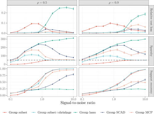
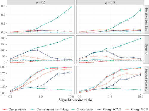
Figure 2 Comparisons of estimators for sparse semiparametric classification. Metrics are aggregated over 30 synthetic datasets generated with n = 1000, p = 10,000, and g = 5000. Solid points represent averages and error bars denote (one) standard errors. Dashed lines indicate the true number of nonzero functions.

Consider first the regression results. In line with our theory, group subset exhibits excellent performance when the signal is strong but fares poorly when the signal is weak. Group lasso behaves contrarily, performing capably at low SNRs but poorly at high SNRs. The transition between the two estimators in terms of relative test loss occurs at $\text{SNR}\approx 2$ in the moderate-correlation scenario ($\rho =0.5$) and later at $\text{SNR}\approx 3$ in the high-correlation scenario ($\rho =0.9$). Group subset + shrinkage achieves the best of both worlds. It improves the performance of group subset when the signal is weak and, by tapering off shrinkage, eventually behaves like group subset when the signal is strong. Group SCAD and group MCP also try to unwind shrinkage via their nonconvexity parameters. Even so, there remains a gap between these estimators and group subset + shrinkage. The latter converges earlier to the right sparsity level and the correct model. The gap is most stark in the high-correlation scenario, where their support recovery is roughly half that of the group subset estimators at $\text{SNR}=10$.

Turning our attention to the classification results, we again see that group lasso maintains an edge in prediction over group subset when the signal is weak and vice-versa when the signal is strong. As before, the gap between group lasso and group subset at low SNRs is closed once shrinkage is introduced. The group subset estimators also continue to have a clear upper hand in support recovery. Closer inspection reveals this upper hand is because they make fewer false positive selections than the competing estimators, similar to the regression setting. There is, however, one interesting difference to the regression setting: group subset + shrinkage has an advantage over group subset when the SNR is high. In this regime, it has noticeably lower relative test loss and marginally better support recovery. This result corresponds to a well-known phenomenon where the maximum likelihood estimator diverges as the classes become separable (see Hastie, Tibshirani, and Wainwright 2015). Shrinkage has the desirable side-effect of preventing this divergence.

5.3 Computational Performance

We now compare the computational performance of grpsel against grpreg for regression. Our estimators—group subset and group subset + shrinkage—and those of grpreg—group lasso, group SCAD, and group MCP—each solve different optimization problems, so it does not make sense to ask whether one implementation is faster than another for the same problem. Rather, the purpose of these comparisons is to provide indications of run time and computational complexity for alternative approaches to structured sparsity. Both grpsel and grpreg are set with a convergence tolerance of ${10}^{-4}$. All run times and iteration counts are measured with reference to the coordinate descent algorithms of each package over a grid of the primary tuning parameter. Where there is a secondary tuning parameter (e.g., the shrinkage parameter in grpsel or nonconvexity parameter in grpreg), the figures reported are averaged over the number of secondary parameter values evaluated. The simulation design is as before, but we now fix the SNR and vary the number of covariates to measure scalability.

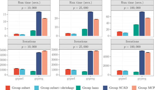
The results as aggregated over 30 synthetic datasets are reported in Figure 3. The vertical bars are averages and the error bars are standard errors. For p = 10,000, grpsel can compute an entire solution path in one to two seconds. Group subset + shrinkage achieves marginally lower run times than group subset, requiring slightly fewer iterations to converge thanks to the additional regularization from shrinkage. For p = 25,000 the run times from grpsel are still less than five seconds to fit a path, while for p = 100,000 the times are around 10 sec. grpreg is also impressive in these scenarios, though relative to grpsel it is slower. Group lasso converges in the fewest iterations, followed by group subset + shrinkage. Group SCAD and group MCP always take several thousand iterations to converge.

Figure 3 Comparisons of grpsel and grpreg, and their estimators. Metrics are aggregated over 30 synthetic datasets generated with $\text{SNR}=1$, $\rho =0.5$, and n = 1000. Vertical bars represent averages and error bars denote (one) standard errors.

Appendix C.2 reports additional computational experiments comparing grpsel with gamsel (Chouldechova and Hastie 2015), an alternative package for sparse semiparametric modeling via overlapping groups and regression splines.

6 Data Analyses

This section studies two contemporary problems: modeling foot traffic in major supermarkets and modeling recessions in the business cycle. Both problems are characterized by the availability of many candidate predictors and the possibility for misspecification of linear models. These characteristics motivate consideration of sparse semiparametric models.

6.1 Supermarket Foot Traffic

The first dataset contains anonymized data on foot traffic and sales volumes for a major Chinese supermarket (see Wang 2009).⁶ The task is to model foot traffic using the sales volumes of different products. To facilitate managerial decision-making, the fitted model should identify a subset of products that well-predict foot traffic (i.e., it should be sparse).

The sample contains n = 464 days. We randomly hold out 10% of the data as a testing set and use the remaining data as a training set. Sales volumes are available for 6398 products. A four-term cubic regression spline is used for each product, resulting in p = 25,592 predictors and g = 12,796 groups (6398 linear groups plus 6398 nonlinear groups). As a measure of predictive accuracy, we report mean square loss on the testing set. We also report the number of fitted functions that are nonzero. As benchmarks, we include random forest and lasso, which respectively produce dense nonparametric models and sparse linear models. In addition, the (unconditional) mean is evaluated as a predictive method to assess the value added by the predictors. 10-fold cross-validation is used to choose tuning parameters.

The metrics under consideration are aggregated over 30 training-testing set splits and reported in Table 1. Averages are reported with standard errors in parentheses. Group subset + shrinkage used to fit sparse semiparametric models leads to the lowest mean square loss, though within statistical precision of group lasso and group MCP. Nonetheless, group subset + shrinkage has the edge of selecting fewer products than either of these estimators, which is advantageous for decision-making. Lasso yields models that are slightly more sparse but at the same time substantially less predictive, signifying linearity might be too restrictive. Random forest is markedly worse than any sparse method. It appears only a small fraction of products explain foot traffic, around 2%–4%.

Table 1 Comparisons of methods for modeling supermarket foot traffic.

		Sparsity
	Mean square loss	Total	Linear	Nonlinear
Group subset + shrinkage	0.650 (0.026)	178.6 (2.3)	115.7 (1.2)	62.9 (2.0)
Group lasso	0.651 (0.025)	267.0 (12.9)	132.9 (2.3)	134.1 (11.0)
Group MCP	0.658 (0.026)	215.1 (6.1)	120.9 (1.2)	94.1 (5.5)
Lasso	0.712 (0.028)	165.2 (5.0)	165.2 (5.0)	–
Random forest	1.330 (0.057)	–	–	–
Mean	9.856 (0.367)	–	–	–

NOTE: Metrics are aggregated over 30 splits of the data into training and testing sets. Averages are reported next to (one) standard errors in parentheses.

6.2 Economic Recessions

The second dataset contains monthly data on macroeconomic series for the United States (see McCracken and Ng 2016).⁷ The dataset is augmented with the National Bureau of Economic Research recession indicator, a dummy variable that indicates whether a given month is a period of recession or expansion.⁸ The task is to model the recession indicator using the macroeconomic series. Such models are useful for scenario analysis and for assessing economic conditions in the absence of low-frequency variables such as quarterly gross domestic product growth.

The sample contains n = 746 months, ending in October 2021. It includes the COVID-19 recession. We again randomly hold out 10% of the data as a testing set and use the remaining data as a training set. Because there are relatively few recessionary periods, a stratified split is applied so that the proportion of recessions in the testing and training sets are equal. The dataset has 127 macroeconomic series. We add to this dataset six lags of each series, leading to a total set of 889 series. Applying a four-term spline to each series yields p = 3556 predictors and g = 1778 groups (889 linear groups plus 889 nonlinear groups). To evaluate predictive accuracy, we report mean logistic loss on the testing set. The remaining metrics and methods are as before.

The results as aggregated over 30 training-testing set splits are reported in Table 2. The sparse semiparametric models from group subset + shrinkage predict recessionary periods well. They perform better than those from group lasso and, at the same time, depend on fewer macroeconomic series. Group MCP is sparser still but also less predictive. Lasso also yields models worse than those from group lasso and group subset + shrinkage, highlighting the value in allowing for nonlinearity. As with the supermarket dataset, the dense models from random forest underperform relative to the sparse models from other methods. All methods improve on the mean, illustrating the predictive content of monthly series.

Table 2 Comparisons of methods for modeling economic recessions.

		Sparsity
	Mean logistic loss	Total	Linear	Nonlinear
Group subset + shrinkage	0.968 (0.103)	44.0 (2.5)	16.2 (0.9)	27.8 (1.8)
Group lasso	1.063 (0.102)	57.5 (1.5)	30.7 (0.7)	26.8 (1.0)
Group MCP	1.141 (0.092)	31.5 (0.7)	18.7 (0.5)	12.8 (0.4)
Lasso	1.093 (0.107)	56.8 (1.1)	56.8 (1.1)	–
Random forest	1.294 (0.039)	–	–	–
Mean	3.703 (0.000)	–	–	–

NOTE: Metrics are aggregated over 30 splits of the data into training and testing sets. Averages are reported next to (one) standard errors in parentheses.

7 Concluding Remarks

Despite a broad array of applications, structured sparsity via group subset selection is not well-studied, especially in high dimensions where it is computationally taxing. This article represents an effort to close the gap. Our optimization framework consists of low complexity algorithms that come with convergence results. A theoretical analysis of the proposed estimators illuminates some of their finite-sample properties. The estimators behave favorably in simulation, exhibiting excellent support recovery when fitting sparse semiparametric models. In real-world modeling tasks, they improve on popular benchmarks.

Supplementary Materials

The supplementary material contains proofs of the theoretical results, additional algorithmic details, and further descriptions and results for the simulations and data analyses.

Data Availability Statement

Our implementation grpsel is available on the R repository CRAN.

Disclosure Statement

The authors report there are no competing interests to declare.

Additional information

Funding

Ryan Thompson’s research was supported by an Australian Government Research Training Program (RTP) Scholarship.

Notes

1 Here and throughout, the intercept term is omitted to facilitate exposition.

2 For all values of the group subset penalty parameter λ0, there exists a constraint parameter s which yields an identical solution.

3 In recent work, Guo, Zhu, and Fan (2021) show that statistical properties of best subset remain valid when the attained minimum is within a certain neighborhood of the global minimum. We expect their analysis extends to structured settings.

4 See also the Julia package ParProx (Ko et al. 2021), which provides tools for memory-efficient structured sparsity.

5 Placing knots at equispaced quantiles is a common knot selection rule (see, e.g., James et al. 2021) that has the benefit of making the spline more flexible in high-density regions while restricting flexibility in low-density regions where less information is available.

6 Available at https://personal.psu.edu/ril4/DataScience.

7 The January 2022 vintage is used, available at https://research.stlouisfed.org/econ/mccracken. See Appendix D.1 of the supplementary material for preprocessing steps.

8 Available at https://fred.stlouisfed.org/series/USREC.

References

- Beck, A., and Eldar, Y. C. (2013), “Sparsity Constrained Nonlinear Optimization: Optimality Conditions and Algorithms,” SIAM Journal on Optimization, 23, 1480–1509. DOI: 10.1137/120869778.
- Beck, A., and Tetruashvili, L. (2013), “On the Convergence of Block Coordinate Descent Type Methods,” SIAM Journal on Optimization, 23, 2037–2060. DOI: 10.1137/120887679.
- Bertsimas, D., and King, A. (2016), “OR Forum—An Algorithmic Approach to Linear Regression,” Operations Research, 64, 2–16. DOI: 10.1287/opre.2015.1436.
- Breheny, P., and Huang, J. (2015), “Group Descent Algorithms for Nonconvex Penalized Linear and Logistic Regression Models with Grouped Predictors,” Statistics and Computing, 25, 173–187. DOI: 10.1007/s11222-013-9424-2.
- Breiman, L. (1996), “Heuristics of Instability and Stabilization in Model Selection,” Annals of Statistics, 24, 2350–2383.
- Chouldechova, A., and Hastie, T. (2015), “Generalized Additive Model Selection,” arXiv: 1506.03850 https://arxiv.org/abs/1506.03850.
- De Mol, C., Giannone, D., and Reichlin, L. (2008), “Forecasting Using a Large Number of Predictors: Is Bayesian Shrinkage a Valid Alternative to Principal Components?” Journal of Econometrics, 146, 318–328. DOI: 10.1016/j.jeconom.2008.08.011.
- Dedieu, A., Hazimeh, H., and Mazumder, R. (2021), “Learning Sparse Classifiers: Continuous and Mixed Integer Optimization Perspectives,” Journal of Machine Learning Research, 22, 1–47.
- Falk, M. (1999), “A Simple Approach to the Generation of Uniformly Distributed Random Variables with Prescribed Correlations,” Communications in Statistics - Simulation and Computation, 28, 785–791. DOI: 10.1080/03610919908813578.
- Fan, J., and Li, R. (2001), “Variable Selection via Nonconcave Penalized Likelihood and its Oracle Properties,” Journal of the American Statistical Association, 96, 1348–1360. DOI: 10.1198/016214501753382273.
- Guo, Y., Berman, M., and Gao, J. (2014), “Group Subset Selection for Linear Regression,” Computational Statistics and Data Analysis, 75, 39–52. DOI: 10.1016/j.csda.2014.02.005.
- Guo, Y., Zhu, Z., and Fan, J. (2021), “Best Subset Selection is Robust Against Design Dependence,” arXiv: 2007.01478 https://arxiv.org/abs/2007.01478.
- Hastie, T., Tibshirani, R., and Tibshirani, R. (2020), “Best Subset, Forward Stepwise or Lasso? Analysis and Recommendations based on Extensive Comparisons,” Statistical Science, 35, 579–592. DOI: 10.1214/19-STS733.
- Hastie, T., Tibshirani, R., and Wainwright, M. (2015), Statistical Learning with Sparsity. The Lasso and Generalizations, Chapman & Hall/CRC Monographs on Statistics and Applied Probability, Boca Raton, FL: CRC Press.
- Hazimeh, H., and Mazumder, R. (2020), “Fast Best Subset Selection: Coordinate Descent and Local Combinatorial Optimization Algorithms,” Operations Research, 68, 1517–1537. DOI: 10.1287/opre.2019.1919.
- Hazimeh, H., Mazumder, R., and Radchenko, P. (2023), “Grouped Variable Selection with Discrete Optimization: Computational and Statistical Perspectives,” Annals of Statistics, 51, 1–32.
- Jacob, L., Obozinski, G., and Vert, J.-P. (2009), “Group Lasso with Overlap and Graph Lasso,” in Proceedings of the 26th International Conference on Machine Learning, pp. 433–440. DOI: 10.1145/1553374.1553431.
- James, G., Witten, D., Hastie, T., and Tibshirani, R. (2021), An Introduction to Statistical Learning (2nd ed), Springer Texts in Statistics, New York: Springer.
- Ko, S., Li, G. X., Choi, H., and Won, J.-H. (2021), “Computationally Scalable Regression Modeling for Ultrahigh-Dimensional Omics Data with ParProx,” Briefings in Bioinformatics, 22, 1–17. DOI: 10.1093/bib/bbab256.
- Li, J., and Chen, W. (2014), “Forecasting Macroeconomic Time Series: Lasso-based Approaches and their Forecast Combinations with Dynamic Factor Models,” International Journal of Forecasting, 30, 996–1015. DOI: 10.1016/j.ijforecast.2014.03.016.
- Lim, M., and Hastie, T. (2015), “Learning Interactions via Hierarchical Group-Lasso Regularization,” Journal of Computational and Graphical Statistics, 24, 627–654. DOI: 10.1080/10618600.2014.938812.
- Lou, Y., Bien, J., Caruana, R., and Gehrke, J. (2016), “Sparse Partially Linear Additive Models,” Journal of Computational and Graphical Statistics, 25, 1026–1040. DOI: 10.1080/10618600.2015.1089775.
- Lounici, K., Pontil, M., van de Geer, S., and Tsybakov, A. B. (2011), “Oracle Inequalities and Optimal Inference Under Group Sparsity,” Annals of Statistics, 39, 2164–2204.
- Mazumder, R., Radchenko, P., and Dedieu, A. (2023), “Subset Selection with Shrinkage: Sparse Linear Modeling When the SNR is low,” Operations Research, 71, 129–147. DOI: 10.1287/opre.2022.2276.
- McCracken, M. W., and Ng, S. (2016), “FRED-MD: A Monthly Database for Macroeconomic Research,” Journal of Business and Economic Statistics, 34, 574–589. DOI: 10.1080/07350015.2015.1086655.
- Meier, L., van de Geer, S., and Bühlmann, P. (2008), “The Group Lasso for Logistic Regression,” Journal of the Royal Statistical Society, Series B, 70, 53–71. DOI: 10.1111/j.1467-9868.2007.00627.x.
- Obozinski, G., Jacob, L., and Vert, J.-P. (2011), “Group Lasso with Overlaps: The Latent Group Lasso Approach,” arXiv: 1110.0413 https://arxiv.org/abs/1110.0413.
- Obozinski, G., Taskar, B., and Jordan, M. (2006), “Multi-Task Feature Selection,” Technical Report. Available at http://citeseerx.ist.psu.edu/viewdoc/download?doi=10.1.1.94.951&rep=rep1&type=pdf.
- Percival, D. (2012), “Theoretical Properties of the Overlapping Groups Lasso,” Electronic Journal of Statistics, 6, 269–288. DOI: 10.1214/12-EJS672.
- Raskutti, G., Wainwright, M. J., and Yu, B. (2011), “Minimax Rates of Estimation for High-Dimensional Linear Regression Over ℓq -Balls,” IEEE Transactions on Information Theory, 57, 6976–6994.
- Ravikumar, P., Lafferty, J., Liu, H., and Wasserman, L. (2009), “Sparse Additive Models,” Journal of the Royal Statistical Society, Series B, 71, 1009–1030. DOI: 10.1111/j.1467-9868.2009.00718.x.
- Rigollet, P. (2015), 18.S997: High dimensional statistics. Lecture notes.
- Simon, N., and Tibshirani, R. (2012), “Standardization and the Group Lasso Penalty,” Statistica Sinica, 22, 983–1001. DOI: 10.5705/ss.2011.075.
- Tibshirani, R. (1996), “Regression Shrinkage and Selection via the Lasso,” Journal of the Royal Statistical Society, Series B, 58, 267–288. DOI: 10.1111/j.2517-6161.1996.tb02080.x.
- Tseng, P. (2001), “Convergence of a Block Coordinate Descent Method for Nondifferentiable Minimization,” Journal of Optimization Theory and Applications, 109, 475–494. DOI: 10.1023/A:1017501703105.
- Wang, H. (2009), “Forward Regression for Ultra-High Dimensional Variable Screening,” Journal of the American Statistical Association, 104, 1512–1524. DOI: 10.1198/jasa.2008.tm08516.
- Yuan, M., and Lin, Y. (2006), “Model Selection and Estimation in Regression with Grouped Variables,” Journal of the Royal Statistical Society, Series B, 68, 49–67. DOI: 10.1111/j.1467-9868.2005.00532.x.
- Zeng, Y., and Breheny, P. (2016), “Overlapping Group Logistic Regression with Applications to Genetic Pathway Selection,” Cancer Informatics, 15, 179–187. DOI: 10.4137/CIN.S40043.
- Zhang, C.-H. (2010), “Nearly Unbiased Variable Selection Under Minimax Concave Penalty,” Annals of Statistics, 38, 894–942.
- Zhang, Y., Zhu, J., Zhu, J., and Wang, X. (2023), “A Splicing Approach to Best Subset of Groups Selection,” INFORMS Journal on Computing 35, 104–119. DOI: 10.1287/ijoc.2022.1241.