Practical application of machine learning for organic matter and harmful algal blooms in freshwater systems: A review

Abstract

The application of machine learning (ML) techniques for understanding and predicting organic matter (OM) and harmful algal blooms (HABs) in freshwater systems has increased significantly with the availability of abundant data and advanced monitoring technologies. However, there is a lack of comprehensive reviews concentrating on practical applications and delving into the potential risks associated with misrepresentation or inflation in constructing ML models. This review aims to bridge these gaps by providing a comprehensive overview of various aspects of ML applications in the context of OM and HABs in freshwater systems. It covers practical ML applications for rapid assessment, early warning, and driver analysis, highlighting the diverse range of techniques employed in these areas. Furthermore, it discusses the challenges and considerations associated with data handling, including using in situ and remote sensing data and the importance of appropriate data-splitting techniques to avoid data leakage. To ensure unbiased and reproducible results, this review offers recommendations for model improvement, such as utilizing explainable ML techniques to gain insights into model behavior and avoiding overreliance on a single ML algorithm. It also emphasizes the significance of deploying ML models through user-friendly interfaces, enabling non-experts in ML to effectively utilize these models in real-world water environments.

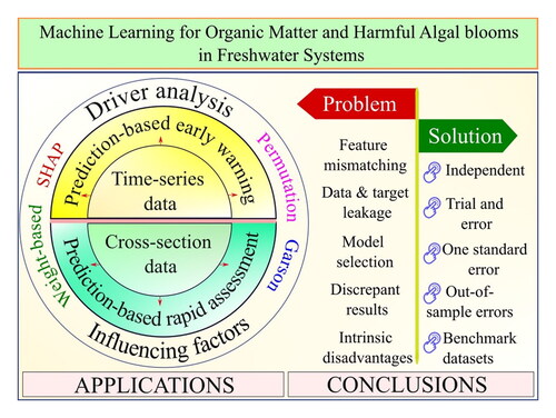
Graphical Abstract

Keywords:

• Algal blooms
• driver analysis
• early warning
• machine learning
• organic matter

HANDLING EDITORS:

• Amit Bhatnagar and Lena Q. Ma

1. Introduction

Freshwater systems, including rivers, lakes, and reservoirs, are invaluable resources for humans, providing irrigation, drinking water, ecological services, and recreational opportunities. Algae, cyanobacteria, and organic matter (OM) play interconnected and significant roles within these systems. The production of OM is closely linked to the growth of phytoplankton and bacteria, particularly during harmful algal blooms (HABs) (Bittar et al., 2015, Du et al., 2022, Tian et al., 2023). Cyanobacteria and algae, in particular, release intracellular OM into the surrounding water upon cell death (Korak et al., 2015, Leloup et al., 2013). Various processes involved in the in situ production and transformation of dissolved organic matter (DOM) in rivers and lakes are closely associated with algal activity or the concentration of Chlorophyll-a (Chl-a) (Herzsprung et al., 2020). Moreover, total organic carbon (TOC) has been identified as a crucial factor in the variation of HABs (Jeong et al., 2022) or Chl-a (Kim & Ahn, 2022). Extensive attention has been devoted to understanding the dynamics, behaviors, and variations of HABs and OM in freshwater systems across different spatial and temporal scales.

Given that algal activity is a biological response to OM and nutrients, and considering that OM in water can manifest biologically (e.g., through microalgal or organism-induced OM), conventional statistical-physics approaches based on thermodynamic equilibrium are inadequate in accurately capturing and forecasting such behaviors. This limitation arises from the inherent complexity, dynamism, or non-equilibrium nature of biologically-induced systems or processes. Thus, data-driven ML methods have emerged as a promising approach to unravel the complexities of OM and the inter-correlations associated with such biological responses, capitalizing on the availability of vast amounts of data (Cichos et al., 2020, James et al., 2017). Recent practical applications of data-driven ML in similar fields include the identification of water sample sources based on physicochemical and microbiological indices (Wang et al., 2021), detection of anomalous cyanobacterial activity in drinking water (Almuhtaram et al., 2021), estimation of DOM photochemical properties (Liao et al., 2023) and phytoplankton concentration (Yu et al., 2021), groundwater quality modeling (Haggerty et al., 2023), identification and prediction of urban water sources (Fu et al., 2022), and tracing microbial source in impaired watersheds (Dubinsky et al., 2016).

While several reviews have discussed the use of ML in water systems, including surface water, groundwater, and seawater, there is a gap in the comprehensive understanding of ML applications in freshwater systems. For instance, Maier et al. (2010) evaluated ML-based models for predicting parameters associated with riverine water resources, specifically focusing on previous studies that used artificial neural networks (ANN). Rajaee and Jafari (2020) reviewed 66 papers published between 2001 and 2019 exploring artificial intelligence models for estimating river sediment quality. Their review focused on data selection, modeling approaches, prediction time steps, and model evaluation. Huang et al. (2021) discussed ML applications for predicting water quality, classifying water resources, tracing contaminant sources, and evaluating pollutant toxicity in rivers, groundwater, lakes, and seawaters. Ortiz-Lopez et al. (2022) summarized the applications of artificial intelligence models in modeling surface water quality, primarily focusing on daily turbidity and pH. Zhu et al. (2022a) provided an overview of surface and drinking water’s general applications, performance, and ML techniques. A review article by Cruz et al. (2021) focused on ML for studying HABs; however, the report specifically discussed potential models and the trends of ML used for forecasting HABs in fresh, brackish, and seawaters. Therefore, there is a notable absence of comprehensive reviews on the application of ML for HABs and OM in freshwater systems.

While previous reviews have made valuable contributions to exploring the applications of ML for various aspects of water systems, such as water quality, sediment, pollutant toxicity, and resources, they have often overlooked the specific areas of OM and HABs. Furthermore, previous reviews have provided general information on ML-based models without delving into the quantitative details of their performance and particular applications. Additionally, these studies have neglected to address crucial aspects of ML optimization, including recommendations for addressing issues such as feature mismatching, target and data leakage, and overfitting. This review addresses these research gaps by providing a comprehensive analysis, quantitative insights, and practical recommendations for optimizing ML applications in freshwater systems, specifically for the study of HABs and OM. The review is tailored to non-experts in ML, offering valuable information that can be applied to address OM or HAB-related issues in their respective freshwater systems.

2. Types of ML applications in freshwater systems

2.1. Classification of practical ML applications

A typical ML project involves gathering a dataset and algorithmically developing a statistical model to address practical tasks. ML can be categorized based on its nature into supervised, unsupervised, and reinforcement learning. Alternatively, it can be classified into techniques such as linear models, neural networks, nonparametric methods, support vector machines (SVMs), and ensemble learning approaches. The majority of ML studies related to OM and HABs, reviewed in this paper, employed supervised learning for predictive modeling. This encompasses both regression (where the output is numeric) and classification (where the outcome is categorical). These ML algorithms exhibit versatility by effectively processing a wide range of data, including structured data (e.g., tabular), unstructured data (e.g., images and text), and time-series data.

We have translated the diverse and intricate nature of ML techniques and data presented in the literature into practical applications (Figure 1). Prior ML research in OM and HABs has predominantly relied on two primary data types: cross-sectional and time series. When paired with specific ML models, these data types serve specialized applications, including rapid assessment, early warning systems, driver analysis, and dynamic insights. Cross-sectional data, collected at a specific point in time, is used to quickly evaluate the status of HABs and OM via ML models. Such models predict aspects of OM and HABs, like concentrations or occurrences, using minimal inputs, thus minimizing laboratory procedures. For example, Goz et al. (2019) and Moradi et al. (2020) utilized data from quick real-time measurements, while Liu et al. (2021) employed remote sensing (RS) data as input variables for predicting DOC. Models trained on one water body may also prove effective for other similar ones, as evidenced by Liu et al. (2022a), who applied an ML model trained with data from Lake Mendota and applied it to Lake Tuesday (US). Furthermore, successful applications of ML models have led to improvements in various fields, including lake management and eco-restoration (Lu et al., 2016), cost reduction (Goz et al., 2019, Nafsin & Li, 2023), public health risk assessment (Lu et al., 2016), mapping spatial–temporal patterns (Sun et al., 2021), and decision-making (Lee et al., 2022, Sagan et al., 2020).

Figure 1. A framework of ML applications for HABs and OM in freshwater systems.

Another frequently used data type in ML research for OM and HABs is time series data, wherein data points are chronologically collected. ML can use time series data to forecast future concentrations or occurrences of OM and HABs in freshwater bodies. Such prediction-based approach enables the development of early warning systems for freshwater systems, supporting efficient decision-making and prompt responses to water pollution incidents, especially in large areas with limited monitoring data. ML models have been trained to effectively capture the time-series patterns and seasonal dynamics of algal cell density, microcystin, and cyanobacteria (Shan et al., 2022, Walter et al., 2001, Zheng et al., 2021). More than just forecasting, these insights explain the inherent mechanisms governing these patterns.

Driver analysis is a technique used to estimate the importance or contribution of independent variables (e.g., water quality, weather conditions) to a response variable (e.g., cyanobacterial, TOC variations) through predictive models or statistical methods. An ML model that effectively represents a target variable can rank feature importance, facilitating the exploration of interrelationships and pinpointing crucial variables associated with the result (Biecek & Burzykowski, 2021). Investigating these controlling factors can assist in policy and water resource decision-making by understanding the cause-and-effect relationships between OM, HABs, and environmental factors (Kim et al., 2019, Lee et al., 2022, Nelson et al., 2018, Park et al., 2015).

2.2. Research trends in previous ML studies

In recent decades, there has been a significant increase in research on ML applications for assessing water quality, monitoring freshwater systems, and managing water resources (Text S1). The number of related publications has risen from 15 in 2012 to 126 in 2022, indicating a growing interest in this field (Figure S1). Through analysis, three main themes or clusters have emerged in these studies: water quality, water management, and river pollution (Figure S2). Among these themes, water quality forecasting has been the most extensively studied area of ML application, followed by water resource management and river water pollution. Other topics, such as environmental monitoring, RS, climate change, watersheds, water levels, water supply, and quality control, have also been explored, although to a lesser extent. It is worth noting that ML for predicting OM or HABs does not appear as a frequently occurring keyword in these studies.

ML models have been employed to predict various parameters related to river water quality, including DO, salinity, EC, biological oxygen demand (BOD), nitrogen (N), algae, and pollutant toxicity, among others (Astuti et al., 2020, Rajaee et al., 2020, Tiyasha et al., 2020). ML has also been used for classifying water resources based on pollution levels, water quality indices, and simulated river sediment, including peak estimation and sediment distribution (Rajaee & Jafari, 2020). Furthermore, ML has supported spatial distribution modeling of water pollutants and identification of pollution sources (Huang et al., 2021, Liu et al., 2022b).

3. ML Applications for management and prediction

3.1. Rapid assessment

3.1.1. Organic matter

Numerous studies have employed ML models to estimate TOC in various water bodies (Table 1). While modern instruments such as conductivity and non-dispersive infrared analyzers are commonly used to detect and quantify TOC accurately, these tools can be expensive. As such, cost-effective and efficient methods like ML are gaining preference (Goz et al., 2019, Kim et al., 2021b). For instance, Goz et al. (2019) developed an ML model to estimate TOC using more affordable input variables (in situ data) such as pH, EC, DO, and WT. Based on the Kernel Extreme Learning Machine (KELM), their model demonstrated remarkable accuracy with an R² value of 0.97, Root Mean Square Error (RMSE) of 0.97 mg/L, and MAPE of 3.01%. Similarly, Kim et al. (2021b) utilized a combination of Multivariate Adaptive Regression Spline (MARS) and M5 Model Tree (M5) to estimate TOC for the Nakdong, Geum, and Yeongsan rivers. Their model used input variables from in situ data, including pH, EC, DO, WT, COD, and SS. The performance of their model was satisfactory, with correlation coefficient (r) and RMSE values of 0.76 and 0.57 mg/L for the Nakdong and Geum Rivers and 0.90 and 0.68 mg/L for the Yeongsan River, respectively.

Table 1. Main characteristics and findings of studies for prediction-based rapid assessment.

Output		Water body	Dataset	Algorithm	Best model	Result (post-resample)	Reference
OM	TOC	Georgia’s streams − 18 watersheds (US)	801	FFNN	FFNN	0.88	Kalin et al. (2010)
	CDOM^qs	Connecticut River	999	LSR & GRNN	GRNN	0.98*	Heddam (2014)
	DOM	NA	1029	KNN, FFNN, SVM, & DT	SVM	87–97***	Cuss et al. (2016)
	CDOM^qs, Chl-a, green algae, & diatoms	River Elbe (Germany)	802–1035	FFNN, SVM, ET, GB, KNN, FSOM, RF, PLSR, & LSR	ET & FFNN	0.88–0.95	Keller et al. (2018)
	TOC	Tersakan stream (Turkey)		FFNN, ELM, KELM, & PLSR	KELM	0.97	Goz et al. (2019)
	DOM & Chl-a	Rappbode Reservoir (Germany)	3641	RF	RF	0.97 and 0.98	Herzsprung et al. (2020)
	DOC (concentration & high events)	Lake Nepean (Australia)	5540 (2002–2018)	LSR, SVR, & GPR	SVM	0.71 (R^2) & 0.92^auc	Moradi et al. (2020)
	FDOM^qs & Chl-a	Two reservoirs & Lake Decatur (US)	200	SVM, DNN, PLSR, & LSTM	SVM & DNN	0.59 & 0.72–0.75	Sagan et al. (2020)
	TOC	Nakdong River (Korea)	389	MARS, M5, & hybrid	Hybrid model	0.76 & 0.90*	Kim et al. (2021b)
	CDOM^ad	Lake Taihu & Qiandaohu (China)	1706	FFNN, SVR, GPR, & RF	GPR	0.74	Sun et al. (2021)
	DOC	Lake Taihu (China)	1316	FFNN	FFNN	15.14**	Liu et al. (2021)
	TOC & Escherichia coli	Milwaukee, Menomonee, & Kinnickinnic rivers (US)	5976	RF, SVM, FFNN, & GBM	FFNN-GBR	0.97 & 0.42	Nafsin and Li (2023)
	DOM	NA	271	GBR, RF, BARD, KNN, & SVM	SVM	0.85 & 0.9	Nguyen et al. (2023)
HABs	Microcystis, Oscillatoria, Phormidiu, Synedra	Lake Kasumigaura (Japan)		FFNN	FFNN	0.35–0.75*	Wei et al. (2001)
	Chl-a	Nakdong River (Korea)	416	LSR & FFNN	FFNN	0.77	Jeong et al. (2006)
	Chl-a	Reservoir Juam (Korea)	2008–2010/2011	FFNN	FFNN	0.85	Cho et al. (2014)
	Chl-a	Lake Poyang (China)	178	FFNN	FFNN	0.59	Huang et al. (2015)
	Chl-a	Lake Champlain (US)	1512	FFNN	FFNN	0.81	Lu et al. (2016)
	PC	Charles River (US)	15849	LSR & FFNN	FFNN	0.9	Heddam (2016)
	Chl-a	Lake Poyang (China)	166	FFNN ensemble models	FFNN	0.26	Huang and Gao (2017)
	Cyanobacteria genera	Lake George (US)	NA	RF	RF	0.13–0.47 (median)	Nelson et al. (2018)
	Chl-a	1087 (2007) & 927 lakes (2012) (US)	411–612	ANFIS types & FFNN	ANFIS & FFNN	0.57–0.85	Luo et al. (2019)
	Chl-a	Englishmen Lake (Spain)	244	FFNN, M5, & SVM	RBF-SVM	0.92	García Nieto et al. (2019)
	Chl-a	Eight lakes (China)	322	XGB & RF	XGB	0.79	Cao et al. (2020)
	Chl-a (water quality & reflectance)	Tri An reservoir (Vietnam)	229	RF, SVM, XGB, CB, & GPR	GPR & CB	0.84 & 0.85	Nguyen et al. (2021)
	Chl-a	45 lakes (China)	273	SVM, LSR, & CB	SVM	0.88	Li et al. (2021)
	Chl-a	Fengshan & Chengcing reservoir (China)	109	RF, DT, & LSR	RF	0.96	Chusnah and Chu (2022)
	Chl-a	Lake Balik (Turkey)	320	CNN, SVM, & MDN	CNN	0.95	Aptoula and Ariman (2022)
	Chl-a	Mid‑Ganga River (India)	105	FFNN & RBFNN	RBFNN	0.98	Bhattacharjee et al. (2022)
	Chl-a	Han river (Korea)	NA	RF, SVM, & FFNN	RF	0.59 & 0.75	Kim and Ahn (2022)
	Chl-a (concentration & seasonal patterns)	Lake Chagan (China)	98	XGB, RF, & KNN	RF	0.79 (F1 0.81)	Shi et al. (2022)
	Chl-a	Xinkai Lake (China)	122	RF	RF	0.89	Xu et al. (2022)
	Chl-a	Dianshan Lake (China)	80	FFNN	FFNN	0.86	Zhu et al. (2022b)
	Chl-a & PC	Geum, Nakdong, & Yeongsan rivers (Korea)	534	CNN	CNN	0.87–0.88*	Hong et al. (2022)
	Chl-a	Erhai Lake (China)	155	SVM, RF, CNN, & ELM	CNN	0.79	Zhao et al. (2022)

Metric result is R² except for * r, ** MAPD, *** accuracy, ^auc Area under the ROC Curve. ^ad: absorption coefficients (1/m); ^fs: field spectroradiometer; ^qs: Quinine sulfate; CNN: Convolutional neural network; RBFNN: Radial basis function neural networks; XGB: Extreme gradient boosting; DT: Decision Tree; KNN: K-nearest neighbors; Kernel ELM; PLST: Partial LSR; GB: Gradient boosting; FSOM: Framework of self-organizing maps; GPR: Gaussian process regression; BARD: Bayesian automatic relevance determination; DNN: Deep neural network.

Moradi et al. (2020) used ML techniques to predict DOC concentrations under various hydrological conditions in the Nepean rivers. They initially employed three ML models (LRS, SVM and Gaussian process regression) to estimate DOC concentration, with the best SVM achieving an R² of 0.71 and RMSE of 1.9 mg/L. The trained ML model successfully identified events with high DOC levels, as indicated by an Area under the Curve (AUC) of 0.92. Liu et al. (2021) applied RS data and a deep learning (DL) model to analyze the spatiotemporal dynamics of DOC concentrations in Lake Taihu, a eutrophic lake in China. Their results indicated that the DL model could estimate the variations of DOC with a Mean Absolute Percent Difference (MAPD) of 15.14%. Furthermore, Heddam (2014) used 999 water samples with input variables such as WT, pH, and EC to estimate the colored dissolved organic matter (CDOM) using the Generalized Regression Neural Network (GRNN) and Least Square Regression (LSR) algorithms. Their study found that the GRNN, with an r of 0.98, outperformed the traditional LSR model, which achieved an r of 0.59.

Various ML techniques have also been utilized for the analysis of DOM using in situ data (Figure 2). Notably, Cuss et al. (2016), Herzsprung et al. (2020), and Nguyen et al. (2023) have leveraged ML to classify DOM sources, predict reactivity classes, and determine source mixing ratios, respectively. Cuss et al. (2016) specifically employed ML to classify DOM derived from different sources based on its fluorescence composition. They reported that the SVM classified entire excitation-emission matrix (EEM) spectra of riverine DOM by source with 87.0–97.2% accuracy. In a separate study, Nguyen et al. (2023) utilized fluorescence EEM data to estimate various sources of DOM in mixed samples under transformative conditions. The authors found that the SVM was the most effective, achieving an R² of 0.85 and 0.9 for soil and compost sources, respectively. Furthermore, Herzsprung et al. (2020) used the Random forest (RF) algorithm to predict reactivity classes in lake and lab-photodegraded DOM samples. They calculated the correlation between the molecular formulae of 60 lakes DOM samples and 13 lab-photodegraded DOM samples. The results revealed that the RF model achieved R² values of 0.97 (Chl-a data) and 0.98 (solar radiation data) in predicting “r,” representing the reactivity classes.

Figure 2. ML applications in rapidly assessing OM and HABs in surface water bodies. (a) Classification of DOM isolated from different sources (leaf leachate and riverine DOM) based on its PARAFAC-modeled fluorescence composition. Reproduced from Cuss et al. (2016) with permission. Copyright (2018) Elsevier. (b) Rapid prediction of cyanobacteria genera using a trained RF model for HAB control in Lake George, US. Reproduced from Nelson et al. (2018) with permission. Copyright (2018) American Chemical Society. (c) Mapping of Chl-a variations in Lake Chaohu, China, created by satellite data and the BST model. Reproduced from Cao et al. (2020) with permission. Copyright (2020) Elsevier. (d) Prediction of nine reactivity classes in lake and lab-photodegraded DOM samples based on the response ratio (r) using an RF model. Reproduced from Herzsprung et al. (2020) with permission. Copyright (2020) American Chemical Society.

3.1.2. Harmful algal blooms

Chl-a and cyanobacteria are widely recognized as common indicators of HABs (Treuer et al., 2021). Standard water quality parameters such as WT, pH, DO, EC, N, and phosphorus (P), along with the weather and hydrologic data including precipitation, temperature, sunshine duration, water level, discharges, and inflows, have been employed as explanatory variables for HABs in ML models (Table 1).

Feedforward Neural Networks (FFNN) and hybrid models have been extensively used to model Chl-a or phytoplankton dynamics for water management and ecological restoration. For example, Lu et al. (2016) determined that an FFNN [7,12,1] was the optimal choice for predicting Chl-a concentrations in Lake Champlain, achieving an R² value of 0.81. In contrast, the bagging-FFNN [7,8,1] yielded only an R² value of 0.26 and a MAPE of 19.7 (Huang & Gao, 2017). In a study comparing FFNN and LSR with different sets of 27 input variables, an FFNN [27,22,1] achieved a higher R² value of 0.77 for estimating phytoplankton dynamics (Jeong et al., 2006).

Efforts have been made to utilize different approaches, including hyperspectral imagery, field reflectance, and satellite data, to quantify Chl-a in water bodies, going beyond the water quality data obtained from laboratory analysis. For instance, Hong et al. (2022) incorporated field monitoring data for Chl-a, field reflectance, and airborne monitoring (RS) in their research. Further, Zhao et al. (2022) estimated Chl-a using field data from small multispectral unmanned aerial vehicles (UAV) and in situ data from ten monitoring stations in Erhai Lake, China.

In addition to detecting variations in Chl-a, measuring other parameters such as phycocyanin (PC) and microorganisms is crucial for understanding the presence of growth of cyanobacteria. Cyanobacteria utilize Chl-a and PC as primary pigments for light absorption and photosynthesis. Several studies have attempted to quantify PC values in inland freshwaters. For instance, Heddam (2016) used 15,849 data points collected at 15-minute intervals to predict PC concentrations in the lower Charles River, USA. The authors proposed an FFNN [4,13,1] model, incorporating inputs such as pH, WT, EC, and DO for the prediction. This model achieved an R² value of 0.98 and a Nash-Sutcliffe Efficiency (NSE) of 0.95, proving more accurate than the LSR models, which reached an R² of 0.89 and an NSE of 0.79. Similarly, Hong et al. (2022) estimated PC concentrations using RS reflectance data and achieved an R² of 0.88.

In other studies focusing on cyanobacteria prediction, Nelson et al. (2018) utilized data from a lake outlet spanning 1993–2010 to estimate the response variable of cyanobacteria genera (Figure 3). They used explanatory variables including N, P, WT, average flow, and partial light extinction coefficient, among others. The RF model achieved NSE values ranging from 0.77 to 0.91 for the training phase and 0.13 to 0.47 for the testing phase. On the other hand, Wei et al. (2001) employed an FFNN [8,40,4] to estimate algal densities of four dominant genera. The trained model achieved a range of r values of 0.67 to 0.75 for Microcystis, Phormidium, and Synedra, while performing less efficiently for Oscillatoria with a low r value of only 0.35.

Figure 3. ML applications for early warning of OM and HABs in freshwater bodies. (a) Combination of daily online monitoring datasets of HABs using buoy sensors for forecasting cyanobacteria cells at 1–6 days ahead in the Siling Reservoir, China, and Lake Winnebago, U.S. Reproduced from Xiao et al. (2017) with permission. Copyright (2017) Elsevier. (b) Comparative results of different ML models for FDOM time series forecasting at 1-hour intervals in Tualatin River, US. Reproduced from Lu and Ma (2020) with permission. Copyright (2020) Elsevier. (c) Forecasting process of the hybrid LSTM model for Chl-a concentration at 1 day, 1 month, and 1 year in advance in Lake Mendota and Tuesday, U.S. Reproduced from Liu et al. (2022a) with permission. Copyright (2022) Elsevier. (d) Comparisons between measured and forecasted cyanobacteria and Microcystis cell counts using the RETAIN model for Yeongsan River, Korea. Reproduced from Kim et al. (2022) with permission. Copyright (2022) Elsevier.

3.2. Early warning

3.2.1. Organic matter

The concentrations of OM, specifically DOC and TOC, fluctuate over time due to various factors such as discharge, meteorological and environmental conditions, and water quality. The trends in DOC concentrations can rapidly change, necessitating high-frequency observations to thoroughly understand the underlying processes (Jones et al., 2014). Factors such as precipitation, vegetation type, soil type, permafrost degradation, and river order influence the spatial distribution of DOC (Liu & Wang, 2022).

Several studies have compared different ML algorithms to identify the most effective models for simulating TOC and fluorescent DOM (FDOM) based on time series data. Yeon et al. (2008) used ML to simulate TOC concentrations in the Pyeongchang River, Korea, during rainy and non-rainy periods at 1-hour and 2-hour intervals. Notably, the models exhibited significant variations in r and RMSE values between rainy and non-rainy seasons. However, despite these variations, all models consistently achieved low RMSE values, ranging from 0.03 to 0.12 mg/L. Fluorescent DOM (FDOM) can serve as a proxy for DOM and has been utilized as a near-real-time monitoring tool for tracking DOM in natural water. FDOM is also a biological indicator of lake water quality (Liu et al., 2019, Yamashita et al., 2010). Lu and Ma (2020) compared the XGBoost (XGB) and RF models for short-term FDOM prediction 1 hour ahead in the Tualatin River, USA. The XGB mode achieved a lower Mean Absolute Percentage Error (MAPE) of 1.59% compared to the RF, which had a MAPE of 2.11%. Green et al. (2021) compared different ML models for forecasting DOC concentrations at 15-minute intervals in streams in the USA. The RF and SVM models used FDOM, turbidity unit (TU), pH, specific conductance, DO, and time as predictors. The results indicated that FDOM had the most significant influence on DOC predictions, with the SVM and RF models achieving NSE values of 0.61 and 0.60, respectively.

3.2.2. Harmful algal blooms

FFNN models have been predominantly utilized for Chl-a predictions (Table 2). For instance, Kim et al. (2019) employed an FFNN to forecast Chl-a in the Nakdong River 1 day in advance. Their study found that the FFNN model, which incorporated wind velocity, EC, alkalinity, N, and dam discharge, exhibited a high R² value of 0.75. Wilson and Recknagel (2001) developed a generic FFNN model to predict algal abundance 1 month in advance in lakes. The model succeeded in two lakes, demonstrating R² values ranging from 0.58 to 0.77, while it produced lower R² values below 0.5 for the other two lakes.

Table 2. Main characteristics and findings of studies for prediction-based early warning.

	Output	Time-ahead	Waterbody	Dataset (Period)	Algorithm	Best model	Result	Reference
OM	TOC	1 & 2 hour	Pyeongchang River (Korea)	NA	ANFIS, MDNN, & FFNN	MDNN	0.67–0.99	Yeon et al. (2008)
	FDOM	1 hour	Tualatin River (US)	1875	XGB & RF	XGB	1.59**	Lu and Ma (2020)
	DOC	15 minutes	Stream (US)	478 (2012–2017)	SVM & RF	SVM	0.61^n	Green et al. (2021)
HABs	Chl-a	7 days	Reservoir	(1979–1982)	RNN	RNN	NA	Walter et al. (2001)
	Chl-a	1 month	Six water bodies (Japan)	(97–375)	FFNN & LSR	FFNN	0.27–0.78*	Wilson and Recknagel (2001)
	Nostocales spp. & Anabaena spp.	3 days	River Darling (Australia)	(1980–1992)	RBFNN	RBFNN	NA	Hou et al. (2006)
	Oscillatoria spp. & Scenedesmus spp.	5 days	Lake Veluwemeer & Wolderwijd (Netherlands)	NA	RNN & HEA	RNN & HEA	0.26–0.9	Talib et al. (2008)
	Chl-a	7 days & 1 year	Nakdong River (Korea)	628 & 857 (1994–2007)	RNN	RNN	0.88 & 0.80	Kim et al. (2012)
	Chl-a	1 month	Lake Baiyangdian (China)	(2000–2009)	FFNN, ARIMA, & LSR	FFNN	0.99	Wang et al. (2013)
	Chl-a	1,3, & 7 days	Hawkesbury River (Australia)	(2004–2009)	FFNN	FFNN	0.98, 0.76 & 0.27	Coad et al. (2014)
	Chl-a	1,3, & 7 days	Hawkesbury River (Australia)	(2004–2009)	FFNN	FFNN	0.98, 0.76 & 0.27	Coad et al. (2014)
	Chl-a	7 days	Yeongsan & Juam reservoir (Korea)	170 (2006–2012)	FFNN & SVM	SVM	0.75 & 0.45	Park et al. (2015)
	Cyanobacteria and Chl-a	1, 2 & 3 days (best)	Siling reservoir (China) & Lake Winnebago (US)	NA	DNN & ARIMA	DNN	0.98–0.99* (cyanobacteria) & 0.87 (Chl-a)	Xiao et al. (2017)
	Chl-a	1 days	Nakdong River (Korea)	259 (2006–2015)	FFNN	FFNN	0.75*	Kim et al. (2019)
	Chl-a	1 year	Dianchi Lake (China)	960 (2005–2012)	LSTM	LSTM	0.63	Yu et al. (2020)
	Algae	10 days	Han River, downstream (Korea)	(2003–2014)	GBM	GBM	0.86^k	Xia et al. (2020)
	Algal bloom alert levels	7 days	Gangjeong-Goryeong reservoir (Korea)	509 (2013–2020)	FFNN & SVM	FFNN	94.8***	Kim et al. (2021a)
	Chl-a (level) & TSI (event)	1 month	Han River (Korea)	(2011–2020)	ANFIS, RNN, LSTM, GRU, SVM, LR, DT, & SARIMAX	ANFIS & RNN	0.93^p	Ly et al. (2021)
	Chl-a	1, 2, & 3 hours	BeiYun River (China)	8399	LSTM	LSTM	0.96–0.99***	Zheng et al. (2021)
	Cyanobacteria, Microcystis, & Aphanizomenon	7 days	Nakdong River & Yeongsan River (Korea)	1827 & 2922 (2013–2020)	LSTM, GRU, & RETAIN	RETAIN	0.76–0.98	Kim et al. (2022)
	Chl-a & HABs	NA	Han, Nakdong, Geum, and Yeongsan rivers (Korea)	1371	CNN & LSTM	CNN	0.66–0.97	Lee et al. (2022)
	HABs	7 days	Eight reservoirs (Korea)	752 (2016–2020)	RF & XGB	RF	0.71–0.93*	Jeong et al. (2022)
	Chl-a	1 hour, 1 day, & 1 month	Lake Mendota & Tuesday (US)	3452 (1995–2020)	LSTM, DNN, & ARIMA	LSTM	0.81–0.98 (level) 92.5–100% (outbreak)	Liu et al. (2022a)
	Chl-a, algal & microcystin	1, 3, & 7 days	Yangtze River (China)	(2014–2018)	LSTM & XGB	LSTM-XGB	0.5–0.91	Shan et al. (2022)

Metric result is R² except for * r, ** MAPE, *** accuracy, ⁿ NSE, ^k Cohen’s Kappa, ^p precision. GRU: gated recurrent unit; SARIMAX: Seasonal autoregressive integrated moving-average model; MDNN: Modular neural network; RETAIN: Reverse time attention; ARIMA: Autoregressive integrated moving average.

Several researchers have combined regression and classification techniques to enhance the effectiveness of ML-based early warning systems. These studies have focused on forecasting HABs and classifying their outbreak levels. For example, Liu et al. (2022a) developed a Long Short-Term Memory (LSTM) to forecast algal blooms in Lake Mendota and Lake Tuesday in the USA. The trained model forecasted Chl-a with R² values of 0.98, 0.88, and 0.81 at hourly, daily, and monthly intervals, respectively. They utilized the model to classify algal outbreaks in Lake Tuesday based on Chl-a, achieving 100% accuracy for Alert Level I (Chl-a ≥ 1 μg/L, early stage of blooms) and 92.5% for Alert Level II (Chl-a ≥ 12 μg/L, severe bloom situation). Similarly, Kim et al. (2021a) classified algal bloom alert levels 7 days in advance in a reservoir. Among the models tested, including SVMs trained on original datasets and FFNN models trained on both original and synthetic-added datasets, the FFNN [13,13,1] model stood out with the highest accuracy of 94.8%. Moreover, Ly et al. (2021) compared various ML models for predicting Chl-a and HABs in the Han River, Korea. In their study, the Adaptive Neuro-Fuzzy Inference System (ANFIS) model attained the lowest mean absolute error (MAE) of 0.107 (mg Chl-a/m³) and the highest precision of 96% for projecting algal outbreak events.

The dynamics of cyanobacteria in water bodies have also been studied using time series data. For instance, Kim et al. (2022) compared three variations of Recurrent Neural Networks (RNN) to predict the populations of different bacterial groups, including Oscillatoria, Anabaena Microcystis, and Aphanizomenon. The study achieved R² values ranging from 0.76 to 0.98 and RMSE values from 0.29 to 1.67 (natural logarithm of cell/mL) across two rivers. In a different research, Talib et al. (2008) utilized Hybrid Evolutionary Algorithms (HEA) and RNNs to predict lakes’ Oscillatoria and Scenedesmus cell counts. The prediction accuracy varied significantly, with R² values ranging from 0.26 to 0.91 for 5-day ahead forecasts of bacterial cells. Other researchers have employed ML techniques for forecasting cyanobacteria cell counts in freshwater bodies. Xiao et al. (2017) demonstrated exceptional performance in predicting 1- to 3-day cyanobacteria cell counts, achieving high r values (0.98–0.99) in the Siling Reservoir. Additionally, Gupta et al. (2023) utilized a surrogate measure based on satellite-derived data to forecast cyanobacterial cell counts at 10-, 20-, and 30-day lead times, yielding an R² range of 0.53–0.61.

4. Influencing factors identified through explainable ML

Various methods, including permutation, weight-based, Garson, and Shapley additive explanations (SHAP), have been utilized for driver analysis to identify influencing factors for HABs or OM (Table 3 and Text S2). Previous studies have commonly investigated water quality parameters and climate factors as essential determinants influencing Chl-a variation. However, results across different studies have shown significant variations, highlighting the complexity of understanding the precise drivers of the target variables. Xia et al. (2020) found that water level and temperature had a stronger influence on river algal blooms than TN and TP concentrations. This was attributed to the already high nutrient levels, which were not the limiting factors for algal growth. Conversely, Deng et al. (2023) observed that both spring climatic factors (such as increasing temperature and decreasing wind speed) and nutrients, particularly total phosphorus, played vital roles in spring blooms in Lake Taihu. These climatic factors emerged as the primary drivers for both bloom areas and frequencies. Kim and Ahn (2022) also reported the significant impact of TP and TN on Chl-a patterns in the Han River basin. Moreover, other studies have confirmed the important role of nutrients in influencing algal blooms. However, they noted that climatic conditions often play an even more crucial role than nutrients in shaping the dynamics of algal blooms (Deng et al., 2023, Nelson et al., 2018). In summary, several parameters have been identified as influencing these dynamics. These include pH (Heddam, 2016, Jeong et al., 2006), wind velocity (Kim et al., 2019), water level (Xia et al., 2020), TOC (Kim & Ahn, 2022), Chl-a (Lee et al., 2022), NO₃-N (Ly et al., 2021), TN (Park et al., 2015), and both water and atmospheric temperature) (Deng et al., 2023, Kim et al., 2022, Xia et al., 2020).

Table 3. Different ML algorithms, techniques and findings of driver analysis.

Method/Technique	Target	Finding (Important orders)	Reference
FFNN (drop-column)	Chl-a	Differed with different models. pH is most important	Jeong et al. (2006)
RNN	Microcystis aeruginosa & Stephanodiscus hantzschii	Changed with different models and prediction time. pH is the most important	Kim et al. (2012)
Spearman correlation	Chl-a	TN, solar radiation, & TP	Park et al. (2015)
FFNN (weights)	PC	pH 37.05 %, SC 28.35 %, WT 21.72 %, & DO 12.86 %	Heddam (2016)
RF (permutation)	Cyanobacteria genera	Changed with different targets. Common: Color, WT,& average flow	Nelson et al. (2018)
SVM (permutation)	Chl-a	Euglenophytes 100%, Dinophlagellata 50%, TP 47%, TU, pH, DO, EC, etc.	García Nieto et al. (2019)
FFNN (weights)	Chl-a	Wind velocity 27.9%, EC 27.5%, alkalinity 18.6%, TN 16.0%, & discharge 10.0%	Kim et al. (2019)
XGB (embedded method)	Chl-a	Near infrared band 50% & Rrc 865/561 ∼ 10%	Cao et al. (2020)
RF (permutation)	Plankthothrix rubescens	WT (3.5) & diatoms (2)	Derot et al. (2020)
RF (permutation)	Chl-a	The number of N atoms, nominal oxidation state, mass, etc.	Herzsprung et al. (2020)
GBM	Chl-a	Differed with different data. Water level & WT were important	Xia et al. (2020)
r & Shannon entropy	Chl-a & algal bloom	NO3-N, DTN, TN, TP (Chl-a); BOD, & temperature (algal bloom)	Ly et al. (2021)
GB (Kernel function) & CB (permutation)	Chl-a	GP: TN, TP, TSS, & PO4-P CB: Band 3 (green) & Band 6 (vegetation red edge)	Nguyen et al. (2021)
FFNN (weights)	Chl-a	Differed from FFNN & RBFNN	Zhao et al. (2021)
CNN (weights)	Chl-a & PC	600 nm, 650 nm, & near-infrared regions	Hong et al. (2022)
XGB & SHAP	HABs	Changed with different rivers	Jeong et al. (2022)
RF	Chl-a	TOC 27%, TN 19%, pH 13%, WT 8%, TP 8%, EC 7%, DO 6%, etc.	Kim and Ahn (2022)
RETAIN (weights)	HABs	Changed with different targets. AT was the most important	Kim et al. (2022)
CNN & SHAP	Chl-a & HABs	Chl-a, DO, WT, & TP	Lee et al. (2022)
RF (normalized score)	TOC & E. coli	TOC target: DOC 58%, BOD5 18%, EC 7%, Chloride 6%, & TS 5%. E.coli target: BOD, DO, TP, temperature, etc.	Nafsin and Li (2023)
RF & XGB, SHAP	Chl-a	The most enhanced-three band, other predictors changed over algorithms	Shi et al. (2022)
Empirical modeling	Cyanobacterial bloom	Wind speed, temperature, & TP	Deng et al. (2023)

Based on variables used in previous studies, the results of feature importance regarding PC pigment variation demonstrated significant variability. For instance, Heddam (2016) identified pH as the most critical variable, contributing 37.5%, followed by SC, WT, and DO. In contrast, Nafsin and Li (2023) highlighted that DOC primarily influenced TOC concentrations, contributing 58%, while BOD and EC played secondary roles at 18% and 7%, respectively. Moreover, Nelson et al. (2018) emphasized that water color and WT exerted a predominant impact on cyanobacteria genera dynamics, with WT being particularly influential on the variation of Planktolyngbya.

Consequently, it becomes apparent that, in addition to nutrient levels, both hydrologic conditions and environmental factors control cyanobacteria dynamics and algal blooms, thereby posing challenges for water managers, mainly due to the uncontrollable nature of many of these factors in the short term (Nelson et al., 2018). It is worth noting that different methods and datasets have yielded diverse findings regarding the critical driver factors influencing OM and HABs in freshwater bodies. The variable importance results for Chl-a variation showed disparities, even when the same method and target variable were used but with different datasets (Xia et al., 2020). Kim et al. (2022) noted differences in the contributions of input features across extra time steps, ranging from 1 to 7 days prior to forecasting. Moreover, the relative importance of variables changed across different rivers (Jeong et al., 2022). These variations underscore the complexity of the drivers influencing OM behavior in freshwater bodies, emphasizing the importance of considering various methods, datasets, and specific contexts when interpreting and comparing results. Moreover, it is essential to highlight that the reported feature importance scores may not be directly comparable across studies due to the different scaling methods employed (Text S3).

5. Data inputs and data splitting

5.1. Data inputs

ML models are versatile and capable of working with diverse data types, encompassing numerical, image, and categorical data. These data can be sourced from both in situ and RS methods, as illustrated in Figure S3. Such data can predominantly be classified into cross-sectional and time series data. In situ data capture a variety of forms, from physical and chemical analyses to sensor measurements and readings obtained from field spectrometers. Conversely, RS data originates from UAVs or satellites and typically comprises reflectance and absorption coefficient measurements derived from a combination of multi-sensors, field spectrometers, and RS methodologies. The merger of historical Landsat data with in situ sampling and contemporary RS sensors has enriched our understanding of long-term bloom dynamics (Ho et al., 2017).

Most studies gathered data on OM and HABs in freshwater environments through in situ analysis. Several research endeavors have strived to assimilate both in situ and RS data when training ML models (Cao et al., 2020, Sagan et al., 2020, Shi et al., 2022, Sun et al., 2021, Xu et al., 2022). For instance, Cao et al. (2020) collected 522 in situ samples from 67 lakes in China and also used data from Landsat 8. The in situ data included Chl-a concentration, absorption coefficients, and reflectance from field spectrometers. They measured reflectance from 350 nm to 1050 nm at each field site and collected surface water samples, while Chl-a concentration was calculated using a spectrophotometer. In another study, Keller et al. (2018) focused on multi-sensor data instead of chemical data. They measured CDOM and algal variables using multi-sensors while incorporating hyperspectral images captured by a hyperspectral snapshot sensor as additional input values.

5.2. Data splitting

The reviewed papers employed six distinct data splitting approaches: Train/Test, Train/Validation/Test, Standard K-fold cross-validation (CV), Train (CV)/Test, Fixed K-fold CV, and Nested K-fold CV (Text S4 and Figure S4). Researchers sometimes use the terms validation and test data interchangeably, which can lead to confusion. For instance, in time series prediction, Coad et al. (2014) partitioned their data into training data from 2004 to 2006, testing data from 2007, and validation data from 2008 to 2009. They treated the validation data as unavailable and used it to evaluate model performance. In another study, Park et al. (2015) utilized a 5-year training dataset from 2006 to 2010 and a 2-year validation dataset from 2011 to 2012.

Commonly, a split ratio of 7:3 or 8:2 is employed. Random splitting is generally used for cross-sectional problems, while intentional splitting is preferred for time-series prediction. Most reviewed studies adhered to the traditional approach of using separate data for model training while reserving test data for evaluation. However, there are exceptions to this approach, such as the study conducted by Xia et al. (2020). Given the limited availability of algal bloom events in their research (i.e., only 12 occurrences out of 102 periods), they used the entire dataset to train the model, employing the k-fold CV method.

6. Algorithms, metrics, and generalization

6.1. Algorithms

In OM research, 39 ML algorithms spanning 178 cases were utilized (Figs. S5 and S6). These algorithms fall into various categories, including neural networks (FFNN, CNN, RNN, LSTM), decision trees (DT, M5), regression methods (LSR, PLSR), ensemble algorithms based on decision trees (RF, XGB, CatBoost, GB), kernel methods (SVM, KELM), fuzzy logic-based systems (ANFIS), time-series forecasting (ARIMA), and evolutionary algorithms (HEA). Each model type has distinct core functionalities; for instance, ARIMA is tailored for time series, while SVM is versatile and capable of handling both time-series forecasting (regression) and classification. Moreover, they differ in data compatibility—CNN is optimal for images, while RNN is suitable for text and time series- and training methods, such as decision trees (like RF and M5) versus gradient descent approaches (like FFNN and SVM). However, these algorithms uniformly underscore the core themes of ML capabilities: predicting outcomes, discerning patterns, and facilitating informed decision-making.

The FFNN models emerged as the most popular algorithm, accounting for approximately 20.6% of use cases. This was followed by RF and SVM, each comprising 11.0%. The LSTM was used in 6.6%, while LSR and Extreme Gradient Boosting (XGB) were each applied in 4.4% of cases. Other models used in more than two cases included Partial Least Squares Regression (PLSR), RNN, Adaptive neuro-fuzzy inference system (ANFIS), Autoregressive Integrated Moving Average (ARIMA), Decision Tree (DT), Gradient Boosting (GB), K-nearest neighbors (KNN), CatBoost (CB), Gated Recurrent Unit (GRU), M5 model tree (M5), and Radial Basis Function Neural Networks (RBFNN) (Figure S5).

The literature demonstrates a wide range of neural network architectures. “FFNN” is used in this review to refer to ANNs with multilayer perceptron structures. These FFNN models employ backpropagation and various activation functions such as sigmoid, hyperbolic, rectified linear, softmax, and Marquardt (Liu et al., 2021, Nafsin & Li, 2023, Xiao et al., 2017). Other types of neural networks include RBFNN, GRNN, CNN, MDNN, and RNN.

RF and SVM have been commonly used in OM and HAB research. RF, a decision tree-based ensemble algorithm, performs well in handling high-dimensional and complex data, such as cyanobacteria and molecular datasets. Similarly, SVM has gained significant attention from ML practitioners due to its strong generalization ability, making it suitable for tasks like pixel-based land cover classification and RS data analysis (Khatami et al., 2016, Kok et al., 2021). These models find extensive application across various fields and data types (Kok et al., 2021, Pereira et al., 2023, Sheykhmousa et al., 2020).

6.2. Evaluation metrics

Thirty-two distinct metrics were utilized to assess the performance of ML models (Figs. S5 and S6). These metrics spanned both regression and classification tasks. Among the 178 cases analyzed, the most commonly employed metrics were RMSE and R², with 38 cases (21.4%) and 36 cases (20.2%), respectively. Other frequently used metrics included MAE at 12.4%, r at 7.7%, MAPE at 6.2%, NSE at 5.1%, and Mean squared error (MSE) at 3.9%.

Metrics such as R², r, and NSE can be categorized as goodness-of-fit metrics. Conversely, a set of metrics, including RMSE, MAE, MAPE, MSE, and Mean Squared Relative Error (MSRE), are commonly used to evaluate the errors of regression models. For classification tasks, metrics such as Accuracy, Recall, AUC, Precision, Bias, TNR (True Negative Rate), and TPR (True Positive Rate) were utilized to assess model performance (Figs. S3b,d).

6.3. Generalization

Most ML models demonstrated high R² values, exceeding 0.7 and forming a long tail in the distribution (Figure 4). The aggregated findings revealed a mean R² of 0.8 for both rapid assessment and early warning tasks. The median R² values were 0.95 for early warning and 0.91 for rapid assessment, indicating a robust predictive performance in both scenarios. Notably, instances of ML models achieving an R² as low as 0.5 were relatively rare, representing outliers within the dataset.

Figure 4. Distribution and R² (r) values for early warning (a) and rapid assessment (b). these include results of different models and datasets. In the case of the same dataset, only the best-performing ML value was collected.

Researchers have proposed rules of thumb for applying metrics in ML practice. For example, Nafsin and Li (2023) suggested that an R² > 0.90 indicates a very satisfactory model, 0.5 < R² < 0.90 indicates a fairly adequate model, and an R² < 0.50 indicates unsatisfactory model performance. Ritter and Muñoz-Carpena (2013) proposed that an NSE exceeding 0.65 could be considered “acceptable.” Furthermore, Lu and Ma (2020) referred to the rule from Lewis (1982) where MAPE below 10% are classified as “excellent,” 10–20% as “good,” 20–50% as “reasonable,” and values exceeding 50% as “inaccurate.”

It is essential to recognize that no metric is flawless, and all model-performance measures have specific limitations (Biecek & Burzykowski, 2021). For instance, while the widely-used R² metric is robust for assessing the explanatory power of a model, some authors have mistakenly interpreted it as a measure of accuracy (Nafsin & Li, 2023, Sun et al., 2021). Notably, R² is sensitive to large values and does not directly reflect the magnitude of errors. Although R² values are often reported, this does not imply that R² is superior to other metrics. Instead, it is a unitless measure that allows intuitive comparisons among studies. Likewise, RMSE is sensitive to outliers, which can affect its reliability in specific scenarios. Consequently, using a combination of different metrics is highly recommended when evaluating an ML model.

Determining the optimal performance in an ML project presents a significant challenge. This is influenced by the specific problem at hand, the dataset, and the project’s objectives (Olson et al., 2017). Benchmark datasets and baseline models are crucial in comparing and selecting appropriate ML tools (Dueben et al., 2022). Numerous studies have adopted baseline models, such as LSR and logistic regression, to compare them with more advanced ML models (Chusnah & Chu, 2022, Heddam, 2016, Herzsprung et al., 2020, Jeong et al., 2006, Kim et al., 2021a, Li et al., 2021). Furthermore, Lu and Ma (2020) employed standard RF and XGB as benchmark references, aiming to assess the enhanced performance potential of hybrid ML models in predicting FDOM.

7. Potential problems and limitations in ML applications

7.1. Feature mismatching and target leakage

Target leakage refers to situations where explanatory variables are not independent of the target variable or serve as proxies for it. For instance, in the study of Nafsin and Li (2023), DOC was used as a predictor variable for TOC. Since DOC is not independent of TOC, this might introduce bias into model performance. Similarly, when predicting Chl-a and CDOM using band combinations as inputs that are highly sensitive to Chl-a/CDOM (Cao et al., 2020, Hong et al., 2022, Nguyen et al., 2021, Shi et al., 2022), it is critical to recognize that these bands may act as proxies for the target parameters, potentially leading to a form of target leakage. However, using these explanatory variables is practical due to their low cost and widespread availability. In such cases, ML techniques should ensure superior performance compared to traditional band-ratio algorithms.

To avoid the risks associated with feature mismatching or target leakage, researchers must thoroughly understand how the target variable is created or calculated and what proxies are available. It is often assumed that explanatory variables are independent; however, this assumption may not always hold. While it is technically possible to apply ML methods even when explanatory variables are correlated, the results may be misleading or unrealistic, as highlighted by Biecek and Burzykowski (2021). Nelson et al. (2018) evaluated various covariates to identify unsuitable variables. They discovered that Chl-a, pheophytin, TSS, and TOC had the potential to serve as proxy indicators of cyanobacteria abundance, which rendered them inappropriate as explanatory variables.

7.2. Model selection

ML models do not represent a “one-size-fits-all” solution, as their performance depends on the specific data and problem. Thus, a “trial and error” approach is often preferred rather than relying on one algorithm. Notably, 29% of the studies reviewed in this analysis employed only one ML model. Additionally, several studies appear to choose models based merely on fundamental metrics such as R², neglecting out-of-sample errors or failing to make comparisons with baseline models. Such an approach could introduce bias into the model selection process.

7.3. Data leakage

Data leakage occurs when information from the test data infiltrates the training data, artificially enhancing the ML model. One common scenario occurs when the distribution of the test data is normalized or scaled to the training dataset. Another case happens when there is an overlap between the groups used for training and testing. The issue of data leakage in the ML model training process can be subtle and hidden, depending on the techniques employed by researchers, which may not always be explicitly disclosed in their studies. For example, several studies did not reveal whether they employed a holdout validation dataset in their ML training (Keller et al., 2018, Sagan et al., 2020, Yeon et al., 2008). Although we cannot explicitly identify which reviewed studies may have encountered data leakage, it is essential to emphasize that it is probable if appropriate precautions are not taken.

7.4. Discrepant results

Many of the studies reviewed have highlighted discrepancies in importance values when different ML techniques are applied to identical datasets (Jeong et al., 2006, Kim et al., 2012, Zhao et al., 2021) or when diverse datasets are used for the same water body (Xia et al., 2020). Such disparities in importance values among ML models can be traced back to the inherent differences in their learning algorithms or techniques (Gevrey et al., 2003). There is a risk that ML might foster erroneous interpretations (Luíza da Costa et al., 2021). Moreover, directly contrasting explanations between two models with distinct structures presents challenges (Biecek & Burzykowski, 2021). Consequently, meticulous attention to algorithms, methods, scores, and interpretation of results is imperative.

7.5. Benchmark datasets

Several benchmark datasets are available for environmental applications, such as streamflow forecasting (Demir et al., 2022), and weather and climate applications (Dueben et al., 2022). However, there is a notable absence of such datasets for OM and HABs in freshwater systems. This deficiency poses a significant challenge for quantitatively comparing diverse ML tools across freshwater ecosystems. Researchers often confront the arduous task of repetitively generating datasets or crafting ML tools from the beginning. Complicating matters, the datasets encompassing a broad spectrum of target variables, including but not limited to CDOM^qs, DOM, TOC, CDOM^ad, Chl-a, green algae, diatoms, and various Cyanobacteria genera.

7.6. Intrinsic disadvantages of ML

In addition to its power, ML has some intrinsic disadvantages in prediction. ML models often require substantial amounts of high-quality data for training. Forecasting the future with ML presumes that the future will follow historical patterns (Chollet & Allaire, 2018). In other words, ML models achieve optimal performance in real-world scenarios only when they have sufficiently learned the diversity and variations of the real world. However, this may not always be readily accessible for all locations or periods related to data limitations. Thus, it is crucial to publish data as open source and provide open-source code to advance ML (Dueben et al., 2022). Leveraging various open datasets makes creating extensive, high-quality training data for ML feasible. Moreover, most ML algorithms are like “black-box” and interpreting them can be challenging. Gaining insights into the underlying biological or environmental factors driving phenomena such as cyanobacteria and Chl-a dynamics through ML tool can also be difficult.

8. Recommendations for proper applications and improvement

The essential steps in ML applications for assessing and predicting OM and HABs are highlighted below and depicted in Figure S7.

1. Data preparation is essential in ML applications (Domingos, 2012). While the exact amount of data required for solving a specific problem remains uncertain, having too few data points (e.g., less than 50 or 100 samples) is generally inadequate when dealing with complex tasks or ML models. As a rough guideline, employing the ten times rule (i.e., collecting a minimum of ten times the number of predictor variables) can assist engineers in applying ML effectively (Hair et al., 2022).

2. Preprocessing is crucial for handling different scales, skewed distributions, and imbalanced data before applying ML. Various methods can be adopted, such as selecting appropriate evaluation metrics and employing resampling techniques to address severely imbalanced data. For instance, adaptive synthetic data generation methods were utilized to address the imbalance in minority class data (Kim et al., 2021a). Other techniques include the min–max scaling method (Shan et al., 2022) and the moving average process (Kim et al., 2012).

3. Using all available data for training without unseen data can lead to inflated results. When variables exhibit internal groupings (i.e., they share similar value levels), standard k-fold CV might lead to information leakage. In such cases, employing a grouped k-fold CV is imperative (Nguyen et al., 2022, Zhang et al., 2020). In a data-rich scenario, it is advisable to randomly divide the dataset into three parts: a training set, a validation set, and a test set. This approach, known as the train-validation-test split, allows for model development, tuning, and final evaluation (Hastie et al., 2009). However, a K-fold CV is suggested in situations with limited data. It is worth noting that holdout CV has limitations since it fails to deploy all available data (Russell & Norvig, 2016).

4. Using out-of-sample errors as a criterion for selecting the best model is strongly encouraged. When comparing models, it is crucial to consider tradeoff analysis, the One standard error rule, statistical confidence interval tests, as well as baseline or benchmark ML models.

5. Certain factors, such as target leakage or the absence of untrained data, can hinder generalization, which refers to model performance on new or unseen data. These issues can lead to inflated generalization results or overfitting. To gain insights into the behavior of black-box ML models and provide explanations, methods like LIME (Ribeiro et al., 2016), SHAP (Lundberg & Lee, 2017) and permutation (Breiman, 2001) should be employed. These techniques offer local and global explanations, shedding light on how the models make predictions.

6. Benchmark and open datasets specifically centered on OM and HABs in freshwater systems are pivotal for advancing research in future applications. Such datasets enable comparisons and mitigate the repeated efforts needed to construct analogous ML datasets from the ground up. A strong recommendation is to foster collaboration among multiple institutions and encourage open data. This will streamline the sharing and accessibility of datasets within the OM and HABs domains. As an initial step, selecting universally recognized targets, such as Chl-a and TOC, would be beneficial as the foundation for these baseline datasets.

7. Lastly, deploying the developed ML model in a user-friendly manner is recommended through a user interface tool. Python and R programming languages offer various packages, allowing for a more straightforward utilization of the ML model.

9. Concluding remarks

After comprehensively synthesizing previous studies that utilized ML for the assessment and prediction of OM and HABs in freshwater systems, the following conclusions can be drawn:

1. Many ML techniques have been employed for source identification, abnormality detection, and clustering of OM and HABs. These ML applications can be classified into prediction-based rapid assessment using cross-sectional data, early warning using time series data, and driver analysis. There is potential for mutual applicability of ML models trained on data from similar water bodies.

2. DOM plays a significant role in the biogeochemical cycling of freshwater ecosystems, and the EEM data associated with DOM contains valuable information. However, investigations of ML for DOM, TOC, and CDOM are not abundant due to limited datasets. Therefore, exploring EEM data using ML holds great promise for uncovering insights into the source apportionment, behavior, and dynamics of DOM in freshwater systems.

3. ML applications have utilized different data types derived from various sources, including in situ and RS data. While data sharing and collaboration in ML applications have been emphasized in many studies, challenges remain in sharing and utilizing this data across different research communities, particularly in OM and HABs, specifically DOM. The unique and complex nature of OM and HABs datasets should be considered when incorporating data from distinct geographic water bodies.

4. FFNN emerged as the most popular algorithm, representing approximately one-fifth of the studies, followed by RF and SVM, with a frequency of 11.0%. However, the prevalence of FFNN does not necessarily indicate its superiority as the best model. Adopting a trial-and-error approach coupled with model selection techniques is highly encouraged.

5. Most ML models performed effectively, with R² values exceeding 0.7. However, it is essential to note that evaluating ML models should not rely solely on one metric.

Abbreviations
AUC	=	Area under the Curve
ANN	=	Artificial Neural Network
ANFIS	=	Adaptive Neuro-Fuzzy Inference System
ARIMA	=	Autoregressive Integrated Moving Average
BOD	=	Biological Oxygen Demand
CB	=	CatBoost
CDOM	=	: Colored Dissolved Organic Matter
Chl-a	=	Chlorophyll a
CNN	=	Convolutional Neural Network
COD	=	Chemical Oxygen Demand
CV	=	Cross-Validation
DO	=	Dissolved Oxygen
DOM	=	Dissolved Organic Matter
DT	=	Decision Tree
EC	=	Electrical Conductivity
ELM	=	Extreme Learning Machine
FDOM	=	Fluorescent Dissolved Organic Matter
FFNN	=	Feedforward Neural Network
GRNN	=	Generalized Regression Neural Network
HABs	=	Harmful Algal Blooms
HEA	=	Hybrid Evolutionary Algorithms
KNN	=	K-Nearest Neighbors
LSR	=	Least Square Regression
M5	=	M5 Model Tree
MAE	=	Mean Absolute Error
MAPE	=	Mean Absolute Percentage Error
MAPD	=	Mean Absolute Percent Difference
ML	=	Machine Learning
NSE	=	Nash-Sutcliffe Efficiency
OM	=	Organic Matter
PC	=	Phycocyanin
PLSR	=	Partial Least Squares Regression
TN	=	Total Nitrogen
TP	=	Total Phosphorus
R	=	Correlation Coefficient
R2	=	Coefficient of Determination
RF	=	Random Forest
RNN	=	Recurrent Neural Networks
RS	=	Remote Sensing
RMSE	=	Root Mean Square Error
SVM	=	Support Vector Machine
TOC	=	Total Organic Carbon
UAV	=	Unmanned Aerial Vehicles
WT	=	Water Temperature
XGB	=	Extreme Gradient Boosting

Disclosure statement

No potential conflict of interest was reported by the author(s).

Additional information

Funding

This work was supported by Development of Source Identification and Apportionment Methods for Toxic Substances in Marine Environments Program of Korea Institute of Marine Science & Technology Promotion (KIMST-20220534) and also by the Development of Living Shoreline Technology based on Blue Carbon Science toward Climate Change Adaptation project of the Korea Institute of Marine Science & Technology Promotion (KIMST-20220526).

References

- Almuhtaram, H., Zamyadi, A., & Hofmann, R. (2021). Machine learning for anomaly detection in cyanobacterial fluorescence signals. Water Research, 197, 117073. https://doi.org/10.1016/j.watres.2021.117073
- Aptoula, E., & Ariman, S. (2022). Chlorophyll-a retrieval from Sentinel-2 images using convolutional neural network regression. IEEE Geoscience and Remote Sensing Letters, 19, 1–5. https://doi.org/10.1109/LGRS.2021.3070437
- Astuti, A. D., Aris, A., Salim, M. R., Azman, S., & Said, M. I. M. (2020). Artificial intelligence approach to predicting river water quality: A review. Journal of Environmental Treatment Techniques, 8, 1093–1100.
- Bhattacharjee, R., Gupta, A., Das, N., Agnihotri, A. K., Ohri, A., & Gaur, S. (2022). Analysis of algal bloom intensification in mid-Ganga river, India, using satellite data and neural network techniques. Environmental Monitoring and Assessment, 194(8), 547. https://doi.org/10.1007/s10661-022-10213-6
- Biecek, P., & Burzykowski, T. (2021). Explanatory model analysis: Explore, explain, and examine predictive models. Chapman and Hall/CRC.
- Bittar, T. B., Vieira, A. A. H., Stubbins, A., & Mopper, K. (2015). Competition between photochemical and biological degradation of dissolved organic matter from the cyanobacteria Microcystis aeruginosa. Limnology and Oceanography, 60(4), 1172–1194. https://doi.org/10.1002/lno.10090
- Breiman, L. (2001). Random forests. Machine Learning, 45(1), 5–32. https://doi.org/10.1023/A:1010933404324
- Cao, Z., Ma, R., Duan, H., Pahlevan, N., Melack, J., Shen, M., & Xue, K. (2020). A machine learning approach to estimate Chlorophyll-a from Landsat-8 measurements in inland lakes. Remote Sensing of Environment, 248, 111974. https://doi.org/10.1016/j.rse.2020.111974
- Cho, S., Lim, B., Jung, J., Kim, S., Chae, H., Park, J., Park, S., & Park, J. K. (2014). Factors affecting algal blooms in a man-made lake and prediction using an artificial neural network. Measurement: Journal of the International Measurement Confederation, 53, 224–233. https://doi.org/10.1016/j.measurement.2014.03.044
- Chollet, F., & Allaire, J. J. (2018). Deep learning with R: Shelter Island. Manning Publications.
- Chusnah, W. N., & Chu, H. J. (2022). Estimating Chlorophyll-a concentrations in tropical reservoirs from band-ratio machine learning models. Remote Sensing Applications: Society and Environment, 25, 100678. https://doi.org/10.1016/j.rsase.2021.100678
- Cichos, F., Gustavsson, K., Mehlig, B., & Volpe, G. (2020). Machine learning for active matter. Nature Machine Intelligence, 2(2), 94–103. https://doi.org/10.1038/s42256-020-0146-9
- Coad, P., Cathers, B., Ball, J. E., & Kadluczka, R. (2014). Proactive management of estuarine algal blooms using an automated monitoring buoy coupled with an artificial neural network. Environmental Modelling & Software, 61, 393–409. https://doi.org/10.1016/j.envsoft.2014.07.011
- Cruz, R. C., Reis Costa, P., Vinga, S., Krippahl, L., & Lopes, M. B. (2021). A review of recent machine learning advances for forecasting harmful algal blooms and shellfish contamination. Journal of Marine Science and Engineering, 9(3), 283. https://doi.org/10.3390/jmse9030283
- Cuss, C. W., McConnell, S. M., & Guéguen, C. (2016). Combining parallel factor analysis and machine learning for the classification of dissolved organic matter according to source using fluorescence signatures. Chemosphere, 155, 283–291. https://doi.org/10.1016/j.chemosphere.2016.04.061
- Demir, I., Xiang, Z., Demiray, B., & Sit, M. (2022). WaterBench-Iowa: A large-scale benchmark dataset for data-driven streamflow forecasting. Earth System Science Data, 14(12), 5605–5616. https://doi.org/10.5194/essd-14-5605-2022
- Deng, J., Shan, K., Shi, K., Qian, S., Zhang, Y., Qin, B., & Zhu, G. (2023). Nutrient reduction mitigated the expansion of cyanobacterial blooms caused by climate change in Lake Taihu according to Bayesian network models. Water Research, 236, 119946. https://doi.org/10.1016/j.watres.2023.119946
- Derot, J., Yajima, H., & Jacquet, S. (2020). Advances in forecasting harmful algal blooms using machine learning models: A case study with Planktothrix rubescens in Lake Geneva. Harmful Algae, 99, 101906. https://doi.org/10.1016/j.hal.2020.101906
- Domingos, P. (2012). A few useful things to know about machine learning. Communications of the ACM, 55(10), 78–87. https://doi.org/10.1145/2347736.2347755
- Du, Y., An, S., He, H., Wen, S., Xing, P., & Duan, H. (2022). Production and transformation of organic matter driven by algal blooms in a shallow lake: Role of sediments. Water Research, 219, 118560. https://doi.org/10.1016/j.watres.2022.118560
- Dubinsky, E. A., Butkus, S. R., & Andersen, G. L. (2016). Microbial source tracking in impaired watersheds using PhyloChip and machine-learning classification. Water Research, 105, 56–64. https://doi.org/10.1016/j.watres.2016.08.035
- Dueben, P. D., Schultz, M. G., Chantry, M., Gagne, D. J., Hall, D. M., & McGovern, A. (2022). Challenges and benchmark datasets for machine learning in the atmospheric sciences: definition, status, and outlook. Artificial Intelligence for the Earth Systems, 1(3), e210002. https://doi.org/10.1175/AIES-D-21-0002.1
- Fu, G., Jin, Y., Sun, S., Yuan, Z., & Butler, D. (2022). The role of deep learning in urban water management: A critical review. Water Research, 223, 118973. https://doi.org/10.1016/j.watres.2022.118973
- García Nieto, P. J., García-Gonzalo, E., Alonso Fernández, J. R., & Díaz Muñiz, C. (2019). Water eutrophication assessment relied on various machine learning techniques: A case study in the Englishmen Lake (Northern Spain). Ecological Modelling, 404, 91–102. https://doi.org/10.1016/j.ecolmodel.2019.03.009
- Gevrey, M., Dimopoulos, I., & Lek, S. (2003). Review and comparison of methods to study the contribution of variables in artificial neural network models. Ecological Modelling, 160(3), 249–264. https://doi.org/10.1016/S0304-3800(02)00257-0
- Goz, E., Yuceer, M., & Karadurmus, E. (2019). Total organic carbon prediction with artificial intelligence techniques. Computer Aided Chemical Engineering, 46, 889–894.
- Green, M. B., Pardo, L. H., Bailey, S. W., Campbell, J. L., McDowell, W. H., Bernhardt, E. S., & Rosi, E. J. (2021). Predicting high-frequency variation in stream solute concentrations with water quality sensors and machine learning. Hydrological Processes, 35(1), e14000. https://doi.org/10.1002/hyp.14000
- Gupta, A., Hantush, M. M., & Govindaraju, R. S. (2023). Sub-monthly time scale forecasting of harmful algal blooms intensity in Lake Erie using remote sensing and machine learning. The Science of the Total Environment, 900, 165781. https://doi.org/10.1016/j.scitotenv.2023.165781
- Haggerty, R., Sun, J., Yu, H., & Li, Y. (2023). Application of machine learning in groundwater quality modeling - A comprehensive review. Water Research, 233, 119745. https://doi.org/10.1016/j.watres.2023.119745
- Hair, J., Hult, G. T. M., Ringle, C., & Sarstedt, M. (2022). A primer on partial least squares structural equation modeling (PLS-SEM). SAGE.
- Hastie, T., Tibshirani, R., & Friedman, J. H. (2009). The elements of statistical learning: Data mining, inference, and prediction. Springer.
- Heddam, S. (2014). Generalized regression neural network (GRNN)-based approach for colored dissolved organic matter (CDOM) retrieval: Case study of Connecticut River at Middle Haddam Station, USA. Environmental Monitoring and Assessment, 186(11), 7837–7848. https://doi.org/10.1007/s10661-014-3971-7
- Heddam, S. (2016). Multilayer perceptron neural network-based approach for modeling phycocyanin pigment concentrations: Case study from lower Charles River buoy, USA. Environmental Science and Pollution Research International, 23(17), 17210–17225. https://doi.org/10.1007/s11356-016-6905-9
- Herzsprung, P., Wentzky, V., Kamjunke, N., Von Tümpling, W., Wilske, C., Friese, K., Boehrer, B., Reemtsma, T., Rinke, K., & Lechtenfeld, O. J. (2020). Improved understanding of dissolved organic matter processing in freshwater using complementary experimental and machine learning approaches. Environmental Science & Technology, 54(21), 13556–13565. https://doi.org/10.1021/acs.est.0c02383
- Ho, J. C., Stumpf, R. P., Bridgeman, T. B., & Michalak, A. M. (2017). Using Landsat to extend the historical record of lacustrine phytoplankton blooms: A Lake Erie case study. Remote Sensing of Environment, 191, 273–285. https://doi.org/10.1016/j.rse.2016.12.013
- Hong, S. M., Cho, K. H., Park, S., Kang, T., Kim, M. S., Nam, G., & Pyo, J. (2022). Estimation of cyanobacteria pigments in the main rivers of South Korea using spatial attention convolutional neural network with hyperspectral imagery. GI Science and Remote Sensing, 59(1), 547–567. https://doi.org/10.1080/15481603.2022.2037887
- Hou, G., Li, H., Recknagel, F., & Song, L. (2006). Modeling phytoplankton dynamics in the river darling (Australia) using the radial basis function neural network. Journal of Freshwater Ecology, 21(4), 639–647. https://doi.org/10.1080/02705060.2006.9664125
- Huang, J., & Gao, J. (2017). An ensemble simulation approach for artificial neural network: An example from Chlorophyll a simulation in Lake Poyang, China. Ecological Informatics, 37, 52–58. https://doi.org/10.1016/j.ecoinf.2016.11.012
- Huang, J., Gao, J., & Zhang, Y. (2015). Combination of artificial neural network and clustering techniques for predicting phytoplankton biomass of Lake Poyang, China. Limnology, 16(3), 179–191. https://doi.org/10.1007/s10201-015-0454-7
- Huang, R., Ma, C., Ma, J., Huangfu, X., & He, Q. (2021). Machine learning in natural and engineered water systems. Water Research, 205, 117666. https://doi.org/10.1016/j.watres.2021.117666
- James, G., Witten, D., Hastie, T., & Tibshirani, R. (2017). An introduction to statistical learning: With applications in R. Springer New York.
- Jeong, B., Chapeta, M. R., Kim, M., Kim, J., Shin, J., & Cha, Y. K. (2022). Machine learning-based prediction of harmful algal blooms in water supply reservoirs. Water Quality Research Journal, 57(4), 304–318. https://doi.org/10.2166/wqrj.2022.019
- Jeong, K. S., Kim, D. K., & Joo, G. J. (2006). River phytoplankton prediction model by Artificial Neural Network: Model performance and selection of input variables to predict time-series phytoplankton proliferations in a regulated river system. Ecological Informatics, 1(3), 235–245. https://doi.org/10.1016/j.ecoinf.2006.04.001
- Jones, T. D., Chappell, N. A., & Tych, W. (2014). First dynamic model of dissolved organic carbon derived directly from high-frequency observations through contiguous storms. Environmental Science & Technology, 48(22), 13289–13297. https://doi.org/10.1021/es503506m
- Kalin, L., Isik, S., Schoonover, J. E., & Lockaby, B. G. (2010). Predicting water quality in unmonitored watersheds using artificial neural networks. Journal of Environmental Quality, 39(4), 1429–1440. https://doi.org/10.2134/jeq2009.0441
- Keller, S., Maier, P. M., Riese, F. M., Norra, S., Holbach, A., Börsig, N., Wilhelms, A., Moldaenke, C., Zaake, A., & Hinz, S. (2018). Hyperspectral data and machine learning for estimating CDOM, Chlorophyll a, diatoms, green algae and turbidity. International Journal of Environmental Research and Public Health, 15(9), 1881. https://doi.org/10.3390/ijerph15091881
- Khatami, R., Mountrakis, G., & Stehman, S. (2016). A meta-analysis of remote sensing research on supervised pixel-based land-cover image classification processes: General guidelines for practitioners and future research. Remote Sensing of Environment, 177, 89–100. https://doi.org/10.1016/j.rse.2016.02.028
- Kim, K. M., & Ahn, J. H. (2022). Machine learning predictions of Chlorophyll-a in the Han river basin, Korea. Journal of Environmental Management, 318, 115636. https://doi.org/10.1016/j.jenvman.2022.115636
- Kim, H. G., Hong, S., Jeong, K. S., Kim, D. K., & Joo, G. J. (2019). Determination of sensitive variables regardless of hydrological alteration in artificial neural network model of Chlorophyll a: Case study of Nakdong River. Ecological Modelling, 398, 67–76. https://doi.org/10.1016/j.ecolmodel.2019.02.003
- Kim, D. K., Jeong, K. S., McKay, R. I. B., Chon, T. S., & Joo, G. J. (2012). Machine learning for predictive management: Short and long term prediction of phytoplankton biomass using genetic algorithm based recurrent neural networks. International Journal of Environmental Research, 6, 96–108.
- Kim, S., Maleki, N., Rezaie-Balf, M., Singh, V. P., Alizamir, M., Kim, N. W., Lee, J.-T., & Kisi, O. (2021b). Assessment of the total organic carbon employing the different nature-inspired approaches in the Nakdong River, South Korea. Environmental Monitoring and Assessment, 193(7), 445. https://doi.org/10.1007/s10661-021-08907-4
- Kim, T., Shin, J., Lee, D., Kim, Y., Na, E., Park, J. H., Lim, C., & Cha, Y. (2022). Simultaneous feature engineering and interpretation: Forecasting harmful algal blooms using a deep learning approach. Water Research, 215, 118289. https://doi.org/10.1016/j.watres.2022.118289
- Kim, J. H., Shin, J. K., Lee, H., Lee, D. H., Kang, J. H., Cho, K. H., Lee, Y. G., Chon, K., Baek, S. S., & Park, Y. (2021a). Improving the performance of machine learning models for early warning of harmful algal blooms using an adaptive synthetic sampling method. Water Research, 207, 117821. https://doi.org/10.1016/j.watres.2021.117821
- Kok, Z. H., Mohamed Shariff, A. R., Alfatni, M. S. M., & Khairunniza-Bejo, S. (2021). Support vector machine in precision agriculture: A review. Computers and Electronics in Agriculture, 191, 106546. https://doi.org/10.1016/j.compag.2021.106546
- Korak, J. A., Wert, E. C., & Rosario-Ortiz, F. L. (2015). Evaluating fluorescence spectroscopy as a tool to characterize cyanobacteria intracellular organic matter upon simulated release and oxidation in natural water. Water Research, 68, 432–443. https://doi.org/10.1016/j.watres.2014.09.046
- Lee, D., Kim, M., Lee, B., Chae, S., Kwon, S., & Kang, S. (2022). Integrated explainable deep learning prediction of harmful algal blooms. Technological Forecasting and Social Change, 185, 122046. https://doi.org/10.1016/j.techfore.2022.122046
- Leloup, M., Nicolau, R., Pallier, V., Yéprémian, C., & Feuillade-Cathalifaud, G. (2013). Organic matter produced by algae and cyanobacteria: Quantitative and qualitative characterization. Journal of Environmental Sciences (China), 25(6), 1089–1097. https://doi.org/10.1016/s1001-0742(12)60208-3
- Lewis, C. D. (1982). Industrial and business forecasting methods: A practical guide to exponential smoothing and curve fitting. Butterworth Scientific.
- Li, S., Song, K., Wang, S., Liu, G., Wen, Z., Shang, Y., Lyu, L., Chen, F., Xu, S., Tao, H., Du, Y., Fang, C., & Mu, G. (2021). Quantification of Chlorophyll-a in typical lakes across China using Sentinel-2 MSI imagery with machine learning algorithm. The Science of the Total Environment, 778, 146271. https://doi.org/10.1016/j.scitotenv.2021.146271
- Liao, Z., Lu, J., Xie, K., Wang, Y., & Yuan, Y. (2023). Prediction of photochemical properties of dissolved organic matter using machine learning. Environmental Science & Technology, 57, 17971–17980. https://doi.org/10.1021/acs.est.2c07545
- Liu, M., He, J., Huang, Y., Tang, T., Hu, J., & Xiao, X. (2022a). Algal bloom forecasting with time-frequency analysis: A hybrid deep learning approach. Water Research, 219, 118591. https://doi.org/10.1016/j.watres.2022.118591
- Liu, W.-X., He, W., Wu, J.-Y., Wu, W.-J., & Xu, F.-L. (2019). Effects of fluorescent dissolved organic matters (FDOMs) on perfluoroalkyl acids (PFAAs) in lake and river water. The Science of the Total Environment, 666, 598–607. https://doi.org/10.1016/j.scitotenv.2019.02.219
- Liu, X., Lu, D., Zhang, A., Liu, Q., & Jiang, G. (2022b). Data-driven machine learning in environmental pollution: gains and problems. Environmental Science & Technology, 56(4), 2124–2133. https://doi.org/10.1021/acs.est.1c06157
- Liu, F., & Wang, D. (2022). Dissolved organic carbon concentration and biodegradability across the global rivers: A meta-analysis. The Science of the Total Environment, 818, 151828. https://doi.org/10.1016/j.scitotenv.2021.151828
- Liu, D., Yu, S., Xiao, Q., Qi, T., & Duan, H. (2021). Satellite estimation of dissolved organic carbon in eutrophic Lake Taihu, China. Remote Sensing of Environment, 264, 112572. https://doi.org/10.1016/j.rse.2021.112572
- Lu, F., Chen, Z., Liu, W., & Shao, H. (2016). Modeling Chlorophyll-a concentrations using an artificial neural network for precisely eco-restoring lake basin. Ecological Engineering, 95, 422–429. https://doi.org/10.1016/j.ecoleng.2016.06.072
- Luíza da Costa, N., Dias de Lima, M., & Barbosa, R. (2021). Evaluation of feature selection methods based on artificial neural network weights. Expert Systems with Applications, 168, 114312. https://doi.org/10.1016/j.eswa.2020.114312
- Lu, H., & Ma, X. (2020). Hybrid decision tree-based machine learning models for short-term water quality prediction. Chemosphere, 249, 126169. https://doi.org/10.1016/j.chemosphere.2020.126169
- Lundberg, S. M., & Lee, S.-I. (2017). A unified approach to interpreting model predictions. Proceedings of the 31st International Conference on Neural Information Processing Systems (pp. 4768–4777). Curran Associates Inc.
- Luo, W., Zhu, S., Wu, S., & Dai, J. (2019). Comparing artificial intelligence techniques for Chlorophyll-a prediction in US lakes. Environmental Science and Pollution Research International, 26(29), 30524–30532. https://doi.org/10.1007/s11356-019-06360-y
- Ly, Q. V., Nguyen, X. C., Lê, N. C., Truong, T. D., Hoang, T. H. T., Park, T. J., Maqbool, T., Pyo, J., Cho, K. H., Lee, K. S., & Hur, J. (2021). Application of machine learning for eutrophication analysis and algal bloom prediction in an urban river: A 10-year study of the Han River, South Korea. The Science of the Total Environment, 797, 149040. https://doi.org/10.1016/j.scitotenv.2021.149040
- Maier, H. R., Jain, A., Dandy, G. C., & Sudheer, K. P. (2010). Methods used for the development of neural networks for the prediction of water resource variables in river systems: Current status and future directions. Environmental Modelling and Software, 25(8), 891–909. https://doi.org/10.1016/j.envsoft.2010.02.003
- Moradi, S., Agostino, A., Gandomkar, Z., Kim, S., Hamilton, L., Sharma, A., Henderson, R., & Leslie, G. (2020). Quantifying natural organic matter concentration in water from climatological parameters using different machine learning algorithms. H2Open Journal, 3(1), 328–342. https://doi.org/10.2166/h2oj.2020.035
- Nafsin, N., & Li, J. (2023). Prediction of total organic carbon and E. coli in rivers within the Milwaukee River basin using machine learning methods. Environmental Science: Advances, 2(2), 278–293. https://doi.org/10.1039/D2VA00285J
- Nelson, N. G., Munoz-Carpena, R., Phlips, E. J., Kaplan, D., Sucsy, P., & Hendrickson, J. (2018). Revealing biotic and abiotic controls of harmful algal blooms in a shallow subtropical lake through statistical machine learning. Environmental Science & Technology, 52(6), 3527–3535. https://doi.org/10.1021/acs.est.7b05884
- Nguyen, H. Q., Ha, N. T., Nguyen-Ngoc, L., & Pham, T. L. (2021). Comparing the performance of machine learning algorithms for remote and in situ estimations of Chlorophyll-a content: A case study in the Tri An Reservoir, Vietnam. Water Environment Research: A Research Publication of the Water Environment Federation, 93(12), 2941–2957. https://doi.org/10.1002/wer.1643
- Nguyen, X. C., Nguyen, T. T. H., Hang, N. T. T., Thai, V. N., Doan, T. O., Duong, T. T., Duong, T. N., Hwang, Y., Lam, V. S., & Ly, Q. V. (2022). Insight into the adsorption of nutrients from water by pyrogenic carbonaceous adsorbents using a bootstrap method and machine learning. ACS ES and T Water, in press. https://doi.org/10.1021/acsestwater.2c00301
- Nguyen, X. C., Seo, Y., Park, H.-Y., Begum, M. S., Lee, B. J., & Hur, J. (2023). Tracking the sources of dissolved organic matter under bio- and photo-transformation conditions using fluorescence spectrum-based machine learning techniques. Environmental Technology & Innovation, 31, 103179. https://doi.org/10.1016/j.eti.2023.103179
- Olson, R. S., La Cava, W., Orzechowski, P., Urbanowicz, R. J., & Moore, J. H. (2017). PMLB: A large benchmark suite for machine learning evaluation and comparison. BioData Mining, 10(1), 36. https://doi.org/10.1186/s13040-017-0154-4
- Ortiz-Lopez, C., Bouchard, C., & Rodriguez, M. (2022). Machine learning models with potential application to predict source water quality for treatment purposes: A critical review. Environmental Technology Reviews, 11(1), 118–147. https://doi.org/10.1080/21622515.2022.2118084
- Park, Y., Cho, K. H., Park, J., Cha, S. M., & Kim, J. H. (2015). Development of early-warning protocol for predicting Chlorophyll-a concentration using machine learning models in freshwater and estuarine reservoirs, Korea. The Science of the Total Environment, 502, 31–41. https://doi.org/10.1016/j.scitotenv.2014.09.005
- Pereira, F. F., Mendes, T. S. G., Simoes, S. J. C., de Andrade, M. R. M., Reiss, M. L. L., Renk, J. F. C., & Santos, T. C. D. (2023). Comparison of LiDAR- and UAV-derived data for landslide susceptibility mapping using Random Forest algorithm. Landslides, 20, 579–600.
- Rajaee, T., & Jafari, H. (2020). Two decades on the artificial intelligence models advancement for modeling river sediment concentration: State-of-the-art. Journal of Hydrology, 588, 125011. https://doi.org/10.1016/j.jhydrol.2020.125011
- Rajaee, T., Khani, S., & Ravansalar, M. (2020). Artificial intelligence-based single and hybrid models for prediction of water quality in rivers: A review. Chemometrics and Intelligent Laboratory Systems, 200, 103978. https://doi.org/10.1016/j.chemolab.2020.103978
- Ribeiro, M. T., Singh, S., & Guestrin, C. (2016). “Why should i trust you?”: Explaining the predictions of any classifier. Proceedings of the 22nd ACM SIGKDD International Conference on Knowledge Discovery and Data Mining (pp. 1135–1144). Association for Computing Machinery.
- Ritter, A., & Muñoz-Carpena, R. (2013). Performance evaluation of hydrological models: Statistical significance for reducing subjectivity in goodness-of-fit assessments. Journal of Hydrology, 480, 33–45. https://doi.org/10.1016/j.jhydrol.2012.12.004
- Russell, S., & Norvig, P. (2016). Artificial intelligence: A modern approach. Pearson.
- Sagan, V., Peterson, K. T., Maimaitijiang, M., Sidike, P., Sloan, J., Greeling, B. A., Maalouf, S., & Adams, C. (2020). Monitoring inland water quality using remote sensing: Potential and limitations of spectral indices, bio-optical simulations, machine learning, and cloud computing. Earth-Science Reviews, 205, 103187. https://doi.org/10.1016/j.earscirev.2020.103187
- Shan, K., Ouyang, T., Wang, X., Yang, H., Zhou, B., Wu, Z., & Shang, M. (2022). Temporal prediction of algal parameters in Three Gorges Reservoir based on highly time-resolved monitoring and long short-term memory network. Journal of Hydrology, 605, 127304. https://doi.org/10.1016/j.jhydrol.2021.127304
- Sheykhmousa, M., Mahdianpari, M., Ghanbari, H., Mohammadimanesh, F., Ghamisi, P., & Homayouni, S. (2020). Support vector machine versus random forest for remote sensing image classification: A meta-analysis and systematic review. IEEE Journal of Selected Topics in Applied Earth Observations and Remote Sensing, 13, 6308–6325. https://doi.org/10.1109/JSTARS.2020.3026724
- Shi, X., Gu, L., Jiang, T., Zheng, X., Dong, W., & Tao, Z. (2022). Retrieval of Chlorophyll-a concentrations using Sentinel-2 MSI imagery in Lake Chagan based on assessments with machine learning models. Remote Sensing, 14(19), 4924. https://doi.org/10.3390/rs14194924
- Sun, X., Zhang, Y., Zhang, Y., Shi, K., Zhou, Y., & Li, N. (2021). Machine learning algorithms for chromophoric dissolved organic matter (Cdom) estimation based on LANDSAT 8 images. Remote Sensing, 13(18), 3560. https://doi.org/10.3390/rs13183560
- Talib, A., Recknagel, F., Cao, H., & van der Molen, D. T. (2008). Forecasting and explanation of algal dynamics in two shallow lakes by recurrent artificial neural network and hybrid evolutionary algorithm. Mathematics and Computers in Simulation, 78(2–3), 424–434. https://doi.org/10.1016/j.matcom.2008.01.037
- Tian, L., Zhang, Z., Wang, Z., Zhang, P., Xiong, C., Kuang, Y., Peng, X., Yu, M., & Qian, Y. (2023). Compositional variations in algal organic matter during distinct growth phases in Karst water. Frontiers in Environmental Science, 11, 1112522. https://doi.org/10.3389/fenvs.2023.1112522
- Tiyasha , Tung, T. M., & Yaseen, Z. M. (2020). A survey on river water quality modelling using artificial intelligence models: 2000–2020. Journal of Hydrology, 585, 124670. https://doi.org/10.1016/j.jhydrol.2020.124670
- Treuer, G., Kirchhoff, C., Lemos, M. C., & McGrath, F. (2021). Challenges of managing harmful algal blooms in US drinking water systems. Nature Sustainability, 4(11), 958–964. https://doi.org/10.1038/s41893-021-00770-y
- Walter, M., Recknagel, F., Carpenter, C., & Bormans, M. (2001). Predicting eutrophication effects in the Burrinjuck Reservoir (Australia) by means of the deterministic model SALMO and the recurrent neural network model ANNA. Ecological Modelling, 146(1–3), 97–113. https://doi.org/10.1016/S0304-3800(01)00299-X
- Wang, C., Mao, G., Liao, K., Ben, W., Qiao, M., Bai, Y., & Qu, J. (2021). Machine learning approach identifies water sample source based on microbial abundance. Water Research, 199, 117185. https://doi.org/10.1016/j.watres.2021.117185
- Wang, F., Wang, X., Chen, B., Zhao, Y., & Yang, Z. (2013). Chlorophyll a simulation in a lake ecosystem using a model with wavelet analysis and artificial neural network. Environmental Management, 51(5), 1044–1054. https://doi.org/10.1007/s00267-013-0029-5
- Wei, B., Sugiura, N., & Maekawa, T. (2001). Use of artificial neural network in the prediction of algal blooms. Water Research, 35(8), 2022–2028. https://doi.org/10.1016/s0043-1354(00)00464-4
- Wilson, H., & Recknagel, F. (2001). Towards a generic artificial neural network model for dynamic predictions of algal abundance in freshwater lakes. Ecological Modelling, 146(1-3), 69–84. https://doi.org/10.1016/S0304-3800(01)00297-6
- Xia, R., Wang, G., Zhang, Y., Yang, P., Yang, Z., Ding, S., Jia, X., Yang, C., Liu, C., Ma, S., Lin, J., Wang, X., Hou, X., Zhang, K., Gao, X., Duan, P., & Qian, C. (2020). River algal blooms are well predicted by antecedent environmental conditions. Water Research, 185, 116221. https://doi.org/10.1016/j.watres.2020.116221
- Xiao, X., He, J., Huang, H., Miller, T. R., Christakos, G., Reichwaldt, E. S., Ghadouani, A., Lin, S., Xu, X., & Shi, J. (2017). A novel single-parameter approach for forecasting algal blooms. Water Research, 108, 222–231. https://doi.org/10.1016/j.watres.2016.10.076
- Xu, S., Li, S., Tao, Z., Song, K., Wen, Z., Li, Y., & Chen, F. (2022). Remote sensing of Chlorophyll-a in Xinkai Lake using machine learning and GF-6 WFV images. Remote Sensing, 14(20), 5136. https://doi.org/10.3390/rs14205136
- Yamashita, Y., Maie, N., Briceño, H., & Jaffé, R. (2010). Optical characterization of dissolved organic matter in tropical rivers of the Guayana Shield, Venezuela. Journal of Geophysical Research: Biogeosciences, 115(G1), G00F10. https://doi.org/10.1029/2009JG000987
- Yeon, I. S., Kim, J. H., & Jun, K. W. (2008). Application of artificial intelligence models in water quality forecasting. Environmental Technology, 29(6), 625–631. https://doi.org/10.1080/09593330801984456
- Yu, P., Gao, R., Zhang, D., & Liu, Z.-P. (2021). Predicting coastal algal blooms with environmental factors by machine learning methods. Ecological Indicators, 123, 107334. https://doi.org/10.1016/j.ecolind.2020.107334
- Yu, Z., Yang, K., Luo, Y., & Shang, C. (2020). Spatial-temporal process simulation and prediction of Chlorophyll-a concentration in Dianchi Lake based on wavelet analysis and long-short term memory network. Journal of Hydrology, 582, 124488. https://doi.org/10.1016/j.jhydrol.2019.124488
- Zhang, K., Zhong, S., & Zhang, H. (2020). Predicting aqueous adsorption of organic compounds onto biochars, carbon nanotubes, granular activated carbons, and resins with machine learning. Environmental Science & Technology, 54(11), 7008–7018. https://doi.org/10.1021/acs.est.0c02526
- Zhao, X., Li, Y., Chen, Y., Qiao, X., & Qian, W. (2022). Water Chlorophyll a estimation using UAV-based multispectral data and machine learning. Drones, 7(1), 2. https://doi.org/10.3390/drones7010002
- Zhao, X., Xu, H., Ding, Z., Wang, D., Deng, Z., Wang, Y., Lu, Z., Wang, G., Wu, T., & Li, W. (2021). Comparing deep learning with several typical methods in prediction of assessing Chlorophyll-a by remote sensing: A case study in Taihu Lake, China. Water Supply, 21(7), 3710–3724. https://doi.org/10.2166/ws.2021.137
- Zheng, L., Wang, H., Liu, C., Zhang, S., Ding, A., Xie, E., Li, J., & Wang, S. (2021). Prediction of harmful algal blooms in large water bodies using the combined EFDC and LSTM models. Journal of Environmental Management, 295, 113060. https://doi.org/10.1016/j.jenvman.2021.113060
- Zhu, W. D., Qian, C. Y., He, N. Y., Kong, Y. X., Zou, Z. Y., & Li, Y. W. (2022b). Research on Chlorophyll-a concentration retrieval based on BP neural network model—Case study of Dianshan Lake, China. Sustainability (Switzerland), 14(14), 8894. https://doi.org/10.3390/su14148894
- Zhu, M., Wang, J., Yang, X., Zhang, Y., Zhang, L., Ren, H., Wu, B., & Ye, L. (2022a). A review of the application of machine learning in water quality evaluation. Eco-Environment & Health, 1(2), 107–116. https://doi.org/10.1016/j.eehl.2022.06.001