Augmented Bifactor Models and Bifactor-(S-1) Models are Identical. A Comment on Zhang, Luo, Zhang, Sun & Zhang (2023)

Abstract

In a recent study, Zhang et al. (2023) proposed the augmented oblique bifactor model as a new methodological contribution, in which an oblique bifactor model is augmented by one or more indicator(s). Zhang et al. (2023) argued that the augmented oblique bifactor model is superior to existing bifactor modeling approaches. In this comment, we show that the augmented oblique bifactor model by Zhang et al. (2023) is identical and therefore indistinguishable from bifactor-(S-1) type of models presented by Eid et al. (2017). The augmentation approach has already been recommended in the original work of Eid et al. (2017) and by Eid (2020). Finally, we highlight strengths of the simulation studies conducted by Zhang et al. (2023), but also show that several of the conclusions drawn by Zhang et al. (2023) are incorrect. We conclude that there are no differences when applying augmented and bifactor-(S-1) type of models.

Keywords:

• Asymmetric bifactor models
• augmented bifactor models
• bifactor-(S*I-1) model
• bifactor-(S-1) model

In a recent article, Zhang et al. (2023) proposed an augmented bifactor model to overcome the identification and convergence problems associated with bifactor (predictive) models. Zhang et al. (2023) presented the augmented oblique bifactor modeling approach as a new and unique modeling approach that had not been presented in the literature before. In two simulation studies, Zhang et al. (2023) studied the performance of the augmentation approach and highlighted its superiority compared to bifactor-(S-1) and bifactor-(S*1-1) models. Zhang et al. (2023) illustrated their approach using real data in which they measured the propensity to take risks and respondents’ attitudes towards entrepreneurship as an outcome variable.

In the present comment, we demonstrate that the augmented oblique bifactor model proposed by Zhang et al. (2023, see Figure 1d) is identical and therefore indistinguishable from the bifactor-(S-1) and bifactor-(S*1-1) models originally proposed by Eid et al. (2017, see their Figure 5) and Eid (2020, see his Figure 2c). We show that the idea of augmenting bifactor models with additional indicators had already been discussed in prior studies (Eid et al., 2017; Eid, 2020) and that there is no statistical or substantive difference between the augmented and the bifactor-(S-1) modeling approach. We also discuss simulation results presented by Zhang et al. (2023) and explain why some of their conclusions regarding the bifactor-(S-1) approach are inadequate and potentially misleading. We believe our comment is necessary because the article by Zhang et al. (2023) contributes to confusion and ambiguity in interpreting latent factors in (asymmetric) bifactor models. Applied researchers may mistakenly assume that the augmented bifactor modeling approach is entirely different from the bifactor-(S*I-1)/bifactor-(S-1) modeling approach, which is not the case, leading to misinterpretation of the factors in these types of models. We want to clarify that the meaning of the factors in these types of bifactor models always depends on the choice of reference (or augmented) indicators, which must be considered whenever relating external variables to the factors in these models. We also explain why the advantages of the augmented oblique bifactor modeling approach, as presented in Zhang et al. (2023), fully apply to the bifactor-(S*I-1)/bifactor-(S-1) modeling approach. Furthermore, we demonstrate that there are no disadvantages to the bifactor-(S*I-1)/bifactor-(S-1) modeling approach when compared to the augmented oblique bifactor modeling approach.

Figure 1. (A) Augmented oblique bifactor model by Zhang et al. (2023) using one augmenting indicator. (B) Bifactor-(S*I-1) model by Eid et al. (2017) with one reference indicator. (C) Augmented orthogonal bifactor model with one augmenting indicator. (D) Bifactor-(S-1) model by Eid et al. (2017) and Eid (2020) with two reference indicators.

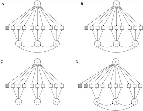
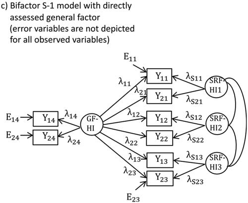
Figure 2. Figure shows a bifactor-(S-1) model in which two additional indicators are used to directly measure general hyperactivity-impulsivity factor (GF-HI) and three specific reference factors for hyperactivity-impulsivity assessed in specific situations (SRF-HI1, SRF-HI2, SRF-HI3). Y_ij: observed variables, E_ij: error variables, λ_ij: factor loadings, i: indicator, j: facet. The above figure was taken from Eid (2020, see his Figure 2c on page 898).

1. Summary of the Study by Zhang et al. (2023)

Zhang et al. (2023) distinguished between orthogonal and oblique bifactor models, with the former restricting the correlations between the specific factors to zero and the latter allowing researchers to freely estimate these correlations. Furthermore, Zhang et al. (2023) discussed augmented and non-augmented bifactor models, where the former include additional augmenting indicators in the model and the latter do not. Figure 1 illustrates four augmented bifactor models. Figure 1A depicts Zhang et al. (2023) proposed augmented oblique bifactor model (see Figure 1d in the article by Zhang et al., 2023). Figure 1B shows Eid et al. (2017) original bifactor-(S*I-1) model with one reference indicator that was added to the model (see Figure 5 in Eid et al., 2017). Figure 1C shows an augmented orthogonal bifactor model with one augmenting indicator (see Figure 1B in Zhang et al., 2023) and Figure 1D shows an augmented oblique bifactor model/bifactor-(S-1) model with two augmented indictors (see Figure 4 in Eid et al., 2017 and Figure 2c in Eid, 2020).

The goal of the study by Zhang et al. (2023) was to overcome the methodological limitations of oblique bifactor models by using the augmentation approach, that is, by adding identifying indicators to the model. The augmentation approach is used to “resolve (approximate) linear dependency between loadings on the general and group factors” (p. 4) and thus facilitates model identification and model convergence. Zhang et al. (2023) argued that the augmentation approach does not only “improve the performance of oblique bifactor measurement models” (p. 4), but also helps “with the estimation of oblique bifactor predictive models” (p. 4), where latent criterion variables are regressed on the general and specific factors in the augmented oblique bifactor model.

Zhang et al. (2023) presented two simulation studies in which they evaluated the statistical performance of the augmentation approach and highlighted its superiority over alternative approaches. In Simulation Study 1, Zhang et al. (2023) examined whether the augmentation approach helps overcome convergence issues of oblique bifactor models without criterion variables. The findings indicated that oblique bifactor models with no augmented indicators suffer from severe convergence problems and yield (in case of convergence) biased results. Zhang et al. (2023) concluded that “one augmenting indicator was sufficient to bring biases of oblique bifactor models to an acceptable level (less than 10%) in most conditions” and that “marginal utility of more augmenting indicators for estimation accuracy was minimal.” (p. 7).

In Simulation Study 2, Zhang et al. (2023) examined the statistical performance of the augmentation approach in the context of predictive models, where the general and specific factors in the bifactor model are used as independent variables to predict a criterion variable. Two data-generating conditions were compared: 1) a condition in which all latent regression coefficients were .25 and 2) a condition in which all latent regression coefficients were zero. In both simulation studies, bifactor models with continuous and categorical indicators were fitted to the data.

In Condition 1 (i.e., all latent regression coefficients were .25), the results revealed that “conditions without augmenting indicators had low convergence rates” and produced severely biased results with respect to the latent regression coefficients (Zhang et al., 2023, p. 9). Again, augmenting bifactor models with one or two additional reference (or identifying) indicators helped to improve the convergence rate, reduce bias, and increase statistical power. In Condition 2, (i.e., all latent regression coefficients were zero 0), “estimation bias was virtually zero across all conditions for both the general factor and the group factors “, except for slightly inflated Type I errors in case of ordered categorical indicators (p. 10). Using real data of N = 391 individuals, Zhang et al. (2023) compared the augmented oblique bifactor modeling approach to classic (oblique and orthogonal) bifactor models. The augmented oblique bifactor model was fitted to data assessing risk taking in five domains, with six indicators for each domain: social, leisure, financial/gambling, health, and ethics. In the predictive bifactor models, respondents’ attitude toward entrepreneurship was used as outcome. In the application, the augmentation approach proved to be a viable solution.

Throughout the article, Zhang et al. (2023) claimed that the augmentation approach is fundamentally distinct from the bifactor-(S*I-1) and bifactor-(S-1) modeling approach presented Eid et al. (2017) and Eid (2020) and that their augmented approach offers greater flexibility and superiority. For example, on p. 5 of their article, Zhang et al. (2023) stated:

We note that the augmentation approach differs from the bifactor-(S-1) and bifactor-(S*I-1) approaches (Eid et al., 2017) in conceptually important ways, despite their statistical similarity. Specifically, the augmentation approach requires the augmenting indicators always be carefully selected before data collection to represent the theoretical meaning of the general factor as adequately as possible (see the Discussion section for how to select augmenting indicators). This strategy “forces” researchers to have an in-depth theorization of the general factor. Once finalized, the augmenting indicators will remain unchanged regardless of who is analyzing the model, thus maintaining the same construct validity across studies (B. Zhang et al., 2023). In contrast, the bifactor-(S-1)/bifactor-(S*I-1) model requires users to choose one group factor/- indicator as a reference factor/indicator and force it to only load on the general factor. This way, in the bifactor-(S-1)/bifactor-(S*I-1) model, the modeled general factor diverges from the theoretical general factor researchers intend to model. Instead, the construct validity of the modeled general factor is equivalent to that of the reference factor/indicator. […] Besides, compared to the bifactor-(S-1)/bifactor-(S*I-1) model, the augmentation approach is more flexible because researchers can choose as many augmenting indicators as needed as long as they can ensure that all the selected indicators adequately represent the general factor and do not tap into any group factors. However, the bifactor-(S-1)/bifactor (S*I-1) model specifically requires users to choose one reference factor/indicator to make the general factor interpretable. If more than one reference factor/indicator is chosen, the interpretability of the model can be compromised.

Zhang et al. (2023, p. 5)

The above quote contains many false and misleading statements, which we will discuss in more detail below. In their discussion, Zhang et al. (2023, Section 5.3) reported the results of a supplementary simulation study in which the bifactor-(S-1) model and a common factor model were fitted to data generated by the traditional oblique bifactor model, based on which Zhang et al. (2023) concluded:

Overall, the simulation suggests that the bifactor-(S-1) approach is not a viable strategy when the data-generating model is a traditional oblique bifactor model. Furthermore, as discussed in the Introduction, compared to the augmentation approach, there may be more issues regarding the construct validity of the general factor and interpretability of the model when the bifactor-(S-1) approach is adopted. Thus, we recommend the use of the augmentation approach for better performance of the oblique bifactor models.

Zhang et al. (2023, p. 15)

In the following, we clarify some inaccuracies and misconception put forth by Zhang et al. (2023) and explain why augmented bifactor models are identical to asymmetric bifactor models such as the bifactor-(S*I-1) and bifactor-(S-1) models proposed by Eid et al. (2017) and Eid (2020).

2. Why is the Augmented Oblique Bifactor Model Indistinguishable from the Bifactor-(S*I-1)/Bifactor-(S-1) Model?

Here, we show that Zhang et al. (2023) augmented oblique bifactor model is mathematically identical and therefore indistinguishable from the bifactor (S*I-1) model presented by Eid et al. (2017) and Eid (2020) if the same reference (or augmenting) indicators are chosen. We already demonstrated the visual equivalence between both models in Figure 1.

Figure 1 illustrates that all models display an asymmetric measurement structure. All models consist of one general factor (G) that has direct effects on all indicators, whereas the specific factors (S_k) only have direct effects on specific indicators that belong to the same facet or domain, except for the reference indicators which are shaded in gray color. The reference indicators – which can equivalently be termed augmenting indicators – only load on the general factor but have no (or zero) loadings on all other specific factors. It is possible to select multiple reference indicators, which yields a bifactor-(S-1) model by Eid et al. (2017) that is illustrated in Figure 1D. Note that the bifactor-(S*I-1) and bifactor-(S-1) models differ only in the number of selected reference indicators.

Furthermore, it is evident that the augmented orthogonal bifactor model (Figure 1C) is simply a restrictive version of the more general bifactor-(S*I-1) model illustrated in Figure 1A and B. In the augmented orthogonal bifactor model (see Figure 1C), the correlations between the specific (group) factors are set to zero, revealing that it is a special case of the bifactor-(S*I-1) model (see Figure 1A and B). This fact was also acknowledged in a prior work by Zhang et al. (2021) in which the authors stated: “The augmented bifactor model (ABiM), which, as detailed in the following, is a more restricted version of the bifactor-(S*I-1) model (Eid et al., 2017), which was also introduced to solve the nonidentification problem” (p. 3).

It is evident that the bifactor (S*I-1) model (see Figure 1B) and the augmented oblique bifactor model (see Figure 1A) are mathematically indistinguishable. When fitted to the same data, both models have identical degrees of freedom, resulting in the same model fit and parameter estimates. This holds true whenever the same reference (or augmenting) indicators are chosen, which determine the psychometric meaning of the factors in these types of models. We will discuss this issue in greater detail below. Confusingly, Zhang et al. (2023) claim that the augmentation approach differs conceptually from the bifactor (S-1) and bifactor (S*I-1) approaches in important ways and that the selection of the augmenting indicators should be guided by theoretical considerations prior to data collection and analysis:

We note that the augmentation approach differs from the bifactor-(S-1) and bifactor-(S*I-1) approaches (Eid et al., 2017) in conceptually important ways, despite their statistical similarity. Specifically, the augmentation approach requires the augmenting indicators always be carefully selected before data collection to represent the theoretical meaning of the general factor as adequately as possible (see the Discussion section for how to select augmenting indicators).

Zhang et al. (2023, p. 5)

This statement is misleading. In Eid et al. (2017), we already recommended that the selection of the reference (marker) indicators should be guided by a priori theoretical considerations and not by the data (see also Eid, 2020). We cautioned against adopting a data-driven approach, a prevalent practice in classical bifactor applications, where researchers frequently encounter anomalous results, such as vanishing specific factors or irregular loading patterns, as summarized in the following paragraph:

The difference between the bifactor-(S*I – 1) model and empirical applications with close-to-zero loadings is that the marker indicator is chosen a priori based on theory in the model, whereas it is data-driven in applications in which one or more indicators do not load significantly onto a specific factor.

Eid et al. (2017, p. 552)

Zhang et al. (2023) do not provide a clear psychometric definition of the factors in the augmented bifactor model. Instead, they offer an intuitive understanding of how they interpret the general factor in their model. Zhang et al. (2023) state that the augmented bifactor model differs from the bifactor-(S-1) and bifactor-(S*I-1) model, because (1) augmenting indicators are added to the model, and (2) they assume that the augmenting indicators only contain general factor variance and measurement error variance, but no method-specific variance. As Zhang et al. (2023) put it:

When the bifactor model (orthogonal or oblique) is used to study hierarchical constructs, researchers have suggested three different approaches to identifying augmenting indicators (B. Zhang et al., 2023). First and maybe the easiest way is to use general indicators that do not refer to any specific target. This approach is particularly suited for hierarchical constructs that involve multiple domains/targets. For example, we can use indicators like “Overall, I am satisfied with my life” or “Overall, I did well on my job” as the augmenting indicators when modeling the general constructs of life satisfaction and job performance which are assessed in multiple dimensions using the bifactor models.

Zhang et al. (2023, p.15/16)

The above statement is problematic in at least two ways. First, in Eid et al. (2017), we have already discussed that selecting one reference facet or one indicator is only one way to apply a bifactor-(S-1) or bifactor-(S*I-1) model. As we noted in Eid et al. (2017), the bifactor-(S-1) and bifactor-(S*I-1) models can also be applied by adding indicators (i.e., augmenting the model) that best represent the g-factor:

The researcher can measure the G factor more directly. For example, in life satisfaction research one could use items that directly target general life satisfaction (i.e., by using a general life satisfaction scale). The common factor pertaining to the general life satisfaction items could be integrated as an independent variable in a model with the specific factors as dependent variables. The regression residuals of the dependent factors would then be interpreted as specific factors in a G factor model. Brunner et al. (2010) have shown how this idea can be applied to the assessment of academic self-concept. The self-assessed general academic self-concept factor is used as an independent variable in predicting the academic self-concept in different domains and domain-specific factors are defined as residual factors that are allowed to be correlated.

Eid et al. (2017, p. 552, emphasis added)

This is exactly identical to what Zhang et al. (2023) presented as the augmentation approach, in which the g-factor is measured directly by additional items that only load on the g-factor and represent the data best. Hence, the augmentation approach is entirely identical to the already existing bifactor-(S-1) modeling approach introduced by Eid et al. (2017). The same approach has already been recommended and applied by Brunner et al. (2010; see, e.g., Figure 1 in Brunner et al.). Adding only one indicator would result in the bifactor-(S*I-1) model (called augmented oblique bifactor model by Zhang et al., 2023). Adding more indicators yields the bifactor-(S-1) model (see Figure 1d). Adding more indicators (items) is what Zhang et al. (2023) propose as an advantage of their approach compared to bifactor-(S-1) modeling approach:

Besides, compared to the bifactor-(S-1)/bifactor-(S*I-1) model, the augmentation approach is more flexible because researchers can choose as many augmenting indicators as needed as long as they can ensure that all the selected indicators adequately represent the general factor and do not tap into any group factors.

Zhang et al. (2023, p. 6)

In recommending the augmentation approach over Eid et al.’s approach, Zhang et al. (2023) even refer to the same example of life satisfaction (highlighted in bold) and give the same recommendation, without referring to the original work by Eid et al. (2017). In addition, Eid (2020) explicitly recommended adding indicators to measure the g-factor directly (“augmentation approach”) when there is not a theoretically outstanding facet that can be used to define the g-factor (see Figure 2c and the decision flow chart in Figure 3 in Eid, 2020).

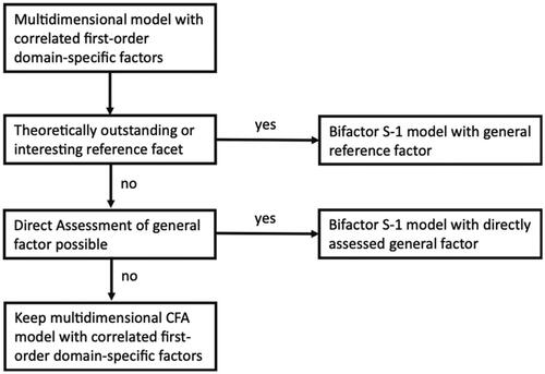
Figure 3. Flowchart taken from Eid (2020, see Figure 2 on page 899).

To emphasize this, we display Figure 2c from Eid (2020) to demonstrate that this model is identical to the augmented oblique bifactor model presented by Zhang et al. (2023, see his Figure 1d). The model in Figure 2 corresponds exactly to the logic of the augmented oblique bifactor model described in the study by Zhang et al. (2023).

Eid (2020) also discusses in detail how bifactor models can be extended by adding items to measure the g-factor directly, particularly in a section entitled “Guidelines for Analyzing Multi-Faceted Constructs with Multidimensional Models” (see point 4):

If there is no outstanding facet but strong assumptions about a reasonable general factor, the general factor can be directly assessed (see Figure 2c). The model in Figure 2c is also a bifactor S-1 model but with the directly assessed general factor as reference factor. If, for example hyperactivity-impulsivity is assessed with respect to the three classes of situations (at school, at home, during sports and exercise) one could add items assessing ADHD/ODD symptoms in general. One could, for example, present the same items with four different instructions assessing the symptoms in general (like the scales used in the study of Burns et al. this issue) and assessing the symptoms in the three different situations. In such an application, the general factor also has a clear meaning (symptoms in general). Moreover, the specific factors indicate to which degree the symptoms in the three situations differ from what can be expected given the general assessment.

Eid (2020, p. 899, emphasis added)

Furthermore, Eid (2020) provides a flow chart (see Figure 3), where the augmentation approach for a direct assessment of the general factor is explicitly represented as another way to apply a bifactor-(S-1) modeling approach.

Zhang et al. (2023) do not credit the work by Eid et al. (2017) or even cite Eid (2020) but presents the augmented oblique bifactor model as a new modeling approach that is supposedly distinct from the bifactor-(S-1) and bifactor-(S*I-1) approach, which is not true. The direct quotes and figures from Eid et al. (2017) and Eid (2020) clearly show that adding items to measure the g-factor directly (e.g., items targeting general life satisfaction or symptoms in general) has been introduced at least 3 years prior to the work by Zhang et al. (2023).

The following statement by Zhang et al. (2023) is therefore incorrect:

In contrast, the bifactor-(S-1)/bifactor-(S*I-1) model requires users to choose one group factor/indicator as a reference factor/indicator and force it to only load on the general factor. This way, in the bifactor-(S-1)/bifactor-(S*I-1) model, the modeled general factor diverges from the theoretical general factor researchers intend to model. Instead, the construct validity of the modeled general factor is equivalent to that of the reference factor/indicator. Moreover, different researchers are likely to choose different group factors/indicators as the reference, leading to fluid construct validity of the general factor and consequently altering the construct validity of all group factors and rendering findings across studies incomparable (see Eid et al., [2017] for an excellent discussion of this issue).

Zhang et al. (2023, pp. 5–6)

The augmented bifactor approach is equivalent to the bifactor-(S*I-1)/bifactor-(S-1) modeling approach by Eid et al. (2017) and has been recommended by Eid et al. (2017, p. 556) and Eid (2020, pp. 898–899). Zhang et al. (2023) must be familiar with at least the Eid et al. (2017) paper as this publication was cited several times in their 2023 article. Therefore, it is irritating that they present the augmentation idea as their own idea, rename the model developed by Eid et al. (2017) present it as a new model, and even devaluate the original model throughout their paper.

3. What Can Be Learned from the Simulation Studies by Zhang et al. (2023)?

The two simulation studies conducted by Zhang et al. (2023) have notable merits as they highlight the advantages and strengths of asymmetric bifactor models, such as bifactor-(S-1) and bifactor-(S*I-1) models. While Zhang et al. (2023) referred to these models as augmented oblique bifactor models in their article, it is important to note that they do not differ from bifactor-(S-1) type of models, as we have shown above. The key conclusion that can be drawn from the simulation studies by Zhang et al. (2023) is that using multiple reference (or augmenting) indicators in asymmetric bifactor models is advisable, as these result in fewer convergence problems and a superior statistical performance in both simulation studies. This is, however, exactly the idea of the bifactor-(S-1) modeling approach, in which multiple reference indicators are used. If Zhang et al. (2023) had acknowledged the equivalence of bifactor-(S-1) type models and the augmented oblique bifactor model in their study and interpreted the simulation results accordingly, the study would be a significant contribution.

However, Zhang et al. (2023) argued against this equivalence and presented the augmented oblique bifactor model as a unique contribution. In Section 5.3, titled “Related Alternative Models” Zhang et al. (2023) presented additional simulations in which they generated data based on an oblique (symmetrical) bifactor model with and without an outcome variable. Then, the bifactor-(S-1) model and a common factor model (including only one general factor) were fitted to the simulated data. The results of this simulation revealed that neither the bifactor-(S-1) model nor the common factor model can accurately recover the coefficients of the predictive oblique bifactor model. Based on this simulation, Zhang et al. (2023) concluded that the bifactor-(S-1) model is generally limited and that the augmented bifactor model should be applied instead.

Overall, the simulation suggests that the bifactor-(S-1) approach is not a viable strategy when the data-generating model is a traditional oblique bifactor model. Furthermore, as discussed in the Introduction, compared to the augmentation approach, there may be more issues regarding the construct validity of the general factor and interpretability of the model when the bifactor-(S-1) approach is adopted. Thus, we recommend the use of the augmentation approach for better performance of the oblique bifactor models.

Zhang et al. (2023, p. 15)

This simulation is problematic as it does not permit a fair evaluation of the bifactor-(S-1) approach. This is because the oblique (symmetrical) bifactor model (i.e., data-generating model) differs fundamentally from the bifactor-(S-1) model (i.e., analysis model). The oblique (symmetrical) bifactor model contains one additional factor (i.e., one specific factor more than the S−1 model). The simulation approach by Zhang et al. (2023) is similar to generating data based on a two-factor model and then fitting a single-factor model to the data. It is impossible for a single-factor model to recover the parameters of a two-factor model, and provided sufficient statistical power, a single-factor model will not fit data generated from a two-factor model. This, however, does not mean that the one-factor model is generally a bad model for empirical social science research. We think that almost all psychometricians would agree.

Following a similar logic, one could easily demonstrate that the augmented oblique bifactor model leads to severely biased estimates when simulating data based on a model in which the augmented indicator(s) share specific variance. In real-world applications, researchers often assume that augmented indicators are free of specific variance (see Zhang et al., 2023), although they cannot be certain that this assumption holds. Under these circumstances, the augmented oblique bifactor model would result in biased estimates, akin to the bifactor-(S-1)/bifactor-(S*I-1) model. Furthermore, if one would simulate data based on the augmented oblique bifactor model and would fit a bifactor-(S-1)/bifactor-(S*I-1) model using the same reference (or augmenting) indicators as in the data-generating augmented oblique bifactor model, there would be no bias at all as compared to the data-generating model, as these models are mathematically identical. This illustrates that the simulation study by Zhang et al. (2023) does not provide a fair comparison and is designed to mislead readers into thinking that bifactor-(S-1)/bifactor-(S*I-1) models are inherently inferior.

In summary, it is not surprising that a bifactor-(S-1) approach will not fit data generated from an oblique (symmetrical) bifactor model well because the models differ in the number of factors. But this does not mean that the bifactor-(S-1) approach is generally deficient or problematic.

4. Discussion

In this article, we commented on a recent article by Zhang et al. (2023). We clarified that the augmented oblique bifactor model does not differ from the bifactor-(S*I-1) model when there is one augmenting indicator, nor does it differ from the bifactor-(S-1) model when multiple augmenting indicators are used. Zhang et al. (2023) augmentation approach results in an asymmetric bifactor model where the augmenting indicators serve as reference indicators in the same manner as in the bifactor-(S-1) approach. Consequently, the psychometric meaning of the g-factor is fully consistent with that of a bifactor-(S-1) model when the same reference indicators are used. Moreover, all other parameters in the augmented oblique factor model, such as the specific factors and their correlations, also depend on the selected augmenting indicators, reflecting the bifactor-(S-1) modeling approach. Therefore, the advantages and limitations of bifactor-(S-1) and bifactor-(S*I-1) models also apply to the augmented oblique bifactor modeling approach, as both modeling approaches are indistinguishable.

In our comment, we also critically examined the simulation studies conducted by Zhang et al. (2023). The primary conclusion that can be drawn from the two main simulation studies reported by Zhang et al. (2023) is that bifactor (S-1) models are effective, powerful, and robust models for addressing several methodological challenges associated with symmetrical bifactor models. The findings also indicate the benefits of incorporating multiple reference indicators in an asymmetric bifactor model, as this can mitigate estimation and convergence issues. When linking outcome variables to the general and specific factors in asymmetric bifactor models, the selection of reference indicators requires careful consideration, as it dictates the interpretation of the factors in the model. Different reference indicators will alter the meaning of the factors in asymmetric bifactor models. This consideration holds true for both bifactor-(S-1) models and augmented bifactor models. As we explained in Eid et al. (2017) and Eid (2020), the selection of reference indicators should be guided by theoretical considerations. We recommend choosing reference indicators that stand out or best represent the construct (e.g., a general life satisfaction scale), that can be considered the gold standard (e.g., by selecting a measure with high validity and reliability), or that have already been used in previous studies to be replicated.

We argue that no superiority of the augmented bifactor modeling approach over the bifactor-(S-1) modeling approach can be claimed, as both approaches are mathematically identical and therefore indistinguishable. As has been explained by Eid et al. (2017), reference indicators can be selected either by adding measures to the model (augmenting the original bifactor model) or by dropping loading or specific factors from the model (reducing the original bifactor model). Therefore, the augmented oblique bifactor model presented by Zhang et al. (2023) is not novel but has already been discussed by Eid et al. (2017).

The final simulation reported by Zhang et al. (2023) does not represent a fair evaluation of the bifactor-(S-1) model, as it was designed in such a way that the bifactor (S-1) model must fail. When fitting the (S-1) model to data generated from an oblique (symmetrical) bifactor model the (S-1) model must yield “biased” parameter estimates relative to the data-generating oblique (symmetrical) bifactor model. In the same way, it would be possible to show that the augmented bifactor model produces biased results when fitted to data generated by an oblique (symmetrical) bifactor model.

We conclude our comment with the following key messages:

• The augmented bifactor modeling approach is indistinguishable from the bifactor-(S-1) modeling approach. When there is a single augmenting indicator, the augmented oblique bifactor model represents a bifactor-(S*I-1) model. In the case of multiple augmenting indicators, it represents a bifactor-(S-1) model. This has been recommended as a possible and worthwhile application by Eid et al. (2017). Zhang et al. (2023) formulated the same recommendation even by referring to exactly the same example (life satisfaction) without citing the source in this context (even though they knew the original paper and cited it in their article).

• Both the augmented and the bifactor-(S-1) modeling approaches result in asymmetric bifactor models utilizing reference (or augmenting) indicators. These indicators determine the psychometric meaning of the general and specific factors in these models.

• Zhang et al. (2023) simulation studies of correctly specified (S-1) models underscore the robustness and effectiveness of asymmetric bifactor models in designs with structurally different facets or domains. The findings suggest that incorporating multiple reference indicators in line with the bifactor-(S-1) modeling approach is advisable.

• The augmented oblique bifactor model is not superior to the bifactor-(S-1) modeling approach but behaves in the same way. Simulations of misspecified models by Zhang et al. (2023) demonstrating different results are constructed in such way that they do not permit a fair and unbiased evaluation.

Correction Statement

This article has been republished with minor changes. These changes do not impact the academic content of the article.

References

- Brunner, M., Keller, U., Dierendonck, C., Reichert, M., Ugen, S., Fisch- bach, A., & Martin, R. (2010). The structure of academic self-concepts revisited: The nested Marsh/Shavelson model. Journal of Educational Psychology, 102, 964–981. http://dx.doi.org/10.1037/a0019644
- Eid, M. (2020). Multi-faceted constructs in abnormal psychology: Implications of the bifactor S-1 model for individual clinical assessment. Journal of Abnormal Child Psychology, 48, 895–900. https://doi.org/10.1007/s10802-020-00624-9
- Eid, M., Krumm, S., Koch, T., & Schulze, J. (2018). Bifactor models for predicting criteria by general and specific factors: Problems of nonidentifiability and alternative solutions. Journal of Intelligence, 6, 42. https://doi.org/10.3390/jintelligence6030042
- Eid, M., Geiser, C., Koch, T., & Heene, M. (2017). Anomalous results in g-factor models: Explanations and alternatives. Psychological Methods, 22, 541–562. https://doi.org/10.1037/met0000083
- Zhang, B., Sun, T., Cao, M., & Drasgow, F. (2021). Using bifactor models to examine the predictive validity of hierarchical constructs: Pros, cons, and solutions. Organizational Research Methods, 24, 530–571. https://doi.org/10.1177/1094428120915522
- Zhang, B., Luo, J., Zhang, S., Sun, T., & Zhang, D. C. (2023). Improving the statistical performance of oblique bifactor measurement and predictive models: An augmentation approach. Structural Equation Modeling: A Multidisciplinary Journal, 31, 233–252. https://doi.org/10.1080/10705511.2023.2222229