A Causal Framework for the Comparability of Latent Variables

Abstract

Measurement invariance (MI) describes the equivalence of measurement models of a construct across groups or time. When comparing latent means, MI is often stated as a prerequisite of meaningful group comparisons. The most common way to investigate MI is multi-group confirmatory factor analysis (MG-CFA). Although numerous guides exist, a recent review showed that MI is rarely investigated in practice. We argue that one reason might be that the results of MG-CFA are uninformative as to why MI does not hold between groups. Consequently, under this framework, it is difficult to regard the study of MI as an interesting and constructive step in the modeling process. We show how directed acyclic graphs (DAGs) from the causal inference literature can guide researchers in reasoning about the causes of non-invariance. For this, we first show how DAGs for measurement models can be translated into path diagrams used in the linear structural equation model (SEM) literature. We then demonstrate how insights gained from this causal perspective can be used to explicitly model encoded causal assumptions with moderated SEMs, allowing for a more enlightening investigation of MI. Ultimately, our goal is to provide a framework in which the investigation of MI is not deemed a “gateway test” that simply licenses further analyses. By enabling researchers to consider MI as an interesting part of the modeling process, we hope to increase the prevalence of investigations of MI altogether.

Keywords:

• Causal inference
• directed acyclic graphs
• measurement invariance
• moderated non-linear factor analysis

With increasingly larger and culturally diverse data sets available, social and behavioral scientists are able to research human experiences and behavior in much broader contexts. For example, extensive studies have been conducted on cultural differences in moral judgement (Bago et al., 2022), prosocial behavior (House et al., 2020), and the values of emotions in societies (Bastian et al., 2014). These new opportunities come with new challenges: we need transparent and objective rules about how to adequately compare groups and under which assumptions we are allowed to generalize results from one group to another. Recently, Deffner et al. (2022) have presented a detailed framework based on causal inference that does just that: Following simple graphical rules of so-called directed acyclic graphs (DAGs), their framework enables researchers to draw inferences and derive licensing assumptions about which comparisons and generalizations are warranted. Researchers working with variables that are observable, like dictator game choices in the examples of Deffner and colleagues, can readily draw on these authors’ framework. However, as Deffner et al. (2022) themselves state, psychologists are often interested in the constructs underlying the observed variables (Westfall & Yarkoni, 2016). As psychologists, we do not care whether you reported you enjoy going out with friends—we care about how extraverted you are. If we use observed variables as direct representations of the underlying construct (e.g., by building a sum score of questionnaire items), we disregard the measurement error inherent in all psychological measures (Lord & Novick, 1968; Van Bork et al., 2022). Ignoring this measurement error in the modeling process can lead to distorted inference. Our model would not be able to distinguish between variation in item responses caused by the construct and variation caused by error (also referred to as unique item variance). Westfall and Yarkoni (2016) for example showed that disregarding measurement error leads to inflated type-I-error rates when trying to statistically control for confounding covariates. As a remedy, they suggest using structural equation models (SEM), which are models that explicitly include the measurement error (Bollen, 1989). In a SEM, constructs are modeled in a measurement model, where a latent variable and the unique error jointly cause the observed variables (Van Bork et al., 2022). Relationships between constructs are modeled in the structural model (Mulaik, 2009). While the use of measurement models allows us to take the measurement error into account, it poses a new challenge for comparisons between groups. In order to be able to meaningfully compare groups, we have to make sure that any difference between groups occurs only due to true differences (i.e., differences in the latent variable), not due to measurement differences (Meuleman et al., 2022). This characteristic is called measurement invariance (MI) and means that the measurement models are equivalent across groups (Meredith, 1993; Putnick & Bornstein, 2016; Vandenberg & Lance, 2000). Although numerous guides (e.g., Putnick & Bornstein, 2016; Van De Schoot et al., 2012) and methods (e.g., Kim et al., 2017) for investigating MI exist, a recent review showed that it is very rarely done in practice (Maassen et al., 2023). The reasons for this are surely diverse. We argue that one reason might be that researchers currently have only little guidance on how to regard the study of MI as an interesting and constructive step in the modeling process. By viewing MI as an informative aspect by itself, we might be able to learn more about psychological constructs. For this, a framework is needed that lets us reason about how and why constructs and measures thereof function differently across groups.

As Deffner et al. (2022) briefly explained, DAGs can be used to depict cases of measurement (non-)invariance. Consequently, DAGs might be a useful tool for reasoning about when latent variables are comparable and generalizable. Our aim is to pick up where Deffner et al. (2022) left off: we want to extend their framework to the case where claims on the construct-level are of interest so that MI is an additional part of the modeling process. The article is structured as follows: First, we briefly introduce the language of DAGs, which are often used in causal inference, and provide a translation to path diagrams for measurement models used in the psychometric SEM literature. Second, we outline the current practice of investigating MI and give a summary of options on how to proceed when MI does not hold. Third, after framing MI as a causal concept, we demonstrate how DAGs can be used to depict non-invariance by encoding assumptions about possible causes of group differences. Fourth, we illustrate in a simulated and an empirical example how following the current practice of investigating MI might miss important aspects of non-invariance. We show how considering the whole causal model instead can help researchers to make more informed modeling choices.

1. From DAGs to Measurement Models

We start by clarifying and defining the terms used throughout this paper. As already mentioned, DAGs are graphical objects used in causal inference to depict causal relationships between variables (Elwert, 2013; Pearl, 1998, 2012). They consist of nodes (the variables) which are connected by edges (directed arrows between these nodes). If a variable is unobserved (latent), we enclose it by a dashed circle. An edge between two variables A and B, denoted by $A\to B,$ means that A has a causal effect on B. DAGs are called directed because only single-headed arrows are allowed,¹ and acyclic because no variable is allowed to be a cause of itself. In general, there are three different causal structures, with which any set of nodes can be described (Deffner et al., 2022; Elwert, 2013; Rohrer, 2018):

• The confounder: $A\leftarrow B\to C,$ that is, the confounder B causes both A and C.

• The chain (psychologists know this as a mediator): $A\to B\to C,$ that is, A causes C through the mediator B.

• The collider: $A\to B\leftarrow C,$ that is, A and C both cause the collider B.

By following the arrows from one variable to another, we can identify the individual paths by which these variables are connected. For all of these constellations exist clear rules of independences between variables (Mulaik, 2009; Pearl, 2012). We say that two variables are conditionally independent if they are unrelated given a (possibly empty) set of other variables. For the confounder and the chain, conditioning on (also: adjusting for) the variable “in the middle” renders the other two variables independent. In this case, we write $A\perp C|B,$ meaning that A and C are independent, conditional on B. For the collider, A and C are unconditionally independent; conditioning on B would in turn render them dependent and produce a non-causal association. Thus, conditioning on a variable closes the path (i.e., “stops the flow of information”) in the case of confounding and mediating variables but opens a non-causal path (i.e., “allows the flow of information”) in the case of colliders (Elwert, 2013). Conditioning can be achieved by including the variable as a predictor in the model but also by specific sampling or experimental designs (Rohrer, 2018). If a path between two variables is closed, the path is said to be d-separated (Pearl, 1988). The risk of conditioning on the “wrong” variable or of missing a variable that should be conditioned on highlights that it is crucial to clearly define the causal relationships between variables prior to analyzing or modeling the data. Failure to do so can lead to spurious associations and distorted inference, for example by accidentally opening paths between variables that should remain closed. We refer readers to Rohrer (2018) and Wysocki et al. (2022) for comprehensive guides on how to approach data analysis from a causal inference perspective.

It is important to note that DAGs depict the causal relationships between a set of random variables without imposing particular distributions or functional forms of the relationships (Greenland & Brumback, 2002; Rohrer, 2018; Suzuki et al., 2020). Their strength lies in making assumptions about the relationships between variables explicit and thereby revealing testable implications between them. That is, if the DAG depicts the true data-generating process, applying the graphical rules of (in)dependences tells us which associations should and should not be observable in the data (Elwert, 2013). Even if a DAG does not fully represent the true data-generating process, it would still be useful because all inferences rely on assumptions and a DAG might help to identify the ones that are otherwise made implicitly. If we are not willing to make any assumptions, no analysis can be reasonably justified (Deffner et al., 2022). In this spirit, when setting up a DAG, it is helpful to view the absence of arrows as strong assumptions and their presence as weak ones (Bollen & Pearl, 2013; Elwert, 2013). An omitted arrow between two variables assumes that the direct causal effect is exactly zero, whereas an arrow assumes some form of relationship without specifying its strength or functional form. Thus, the less we are certain about relationships between variables, the more arrows we should draw.

To bridge the gap between DAGs and path diagrams for SEM—and more specifically, measurement models—it is helpful to view DAGs as non-parametric SEMs (Bollen & Pearl, 2013; Pearl, 2012). A non-parametric SEM is a model in which we do not make assumptions about the functional form of the associations between variables. Consider the DAG of a simple measurement model in Figure 1.

Figure 1. Simple DAG of a measurement model where the observed variables $Y_1,$ $Y_2,$ and $Y_3$ are caused by a latent common factor C and latent unique error terms $E_1,$ $E_2,$ and $E_3.$

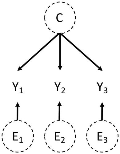
The observed variables $Y_1,$ $Y_2,$ and $Y_3$ are caused by the unobserved (latent) variables C and $E_1,$ $E_2,$ and $E_3.$ C is called the common factor and interpreted as a common cause of $Y_{1-3}$ (Van Bork et al., 2022). Each Y also has its unique cause E that is independent of C. Interpreting this DAG as a non-parametric SEM, we can formally describe the vector of observed variables $\mathit{Y}$ as $\mathit{Y}=f(C,\mathit{E}).$ Typically, when dealing with SEMs, we assume that the relationships are linear and that the variables follow certain distributions. This gives rise to the equation for measurement models in SEM (Mulaik, 2010)²: (1) $$\mathit{Y}=\mathit{\tau }+\mathbf{\Lambda }C+\mathit{E}$$(1)

Here, $\mathbf{\Lambda }$ is the matrix of path coefficients (called loadings), quantifying the strength of the relationship between the observed variables $\mathit{Y}$ and the latent variable C, $\mathit{\tau }$ is the vector of intercepts of $\mathit{Y},$ and $\mathit{E}$ is the vector of unique error terms of $\mathit{Y}$ which cannot be explained by C. In addition to this structural assumption, the following distributional assumptions are often made for estimation purposes: $C\sim N(\alpha ,\Phi )$ and $\mathit{E}\sim \mathit{\text{MVN}}(0,\mathbf{\Psi }).$ $\alpha$ and $\Phi$ are the expectation and the variance of C, respectively. The variances of the errors $\mathit{E}$ are captured on the diagonal of $\mathbf{\Psi }$ (usually, errors are assumed to be uncorrelated, so the off-diagonal entries of $\mathbf{\Psi }$ are 0). The covariance of the data is defined as $\mathbf{\Sigma }=\mathbf{\Lambda }\mathbf{\Phi }{\mathbf{\Lambda }}^{\top }+\mathbf{\Psi }$ (Jöreskog, 1967); that is, variation in the data can be decomposed into a part that is explained by the common factor and an error part.

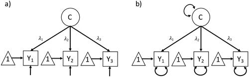
The assumption of linearity lets us now translate our measurement model from a DAG (Figure 1) to a path diagram (Figure 2), which is a common form of diagram in the psychological literature (see Epskamp, 2015 for definitions and visualizations of different styles of path diagrams). Latent variables (in our case: C) are enclosed by a circle. Error terms (in our case: E) are not included explicitly. Instead, their variances are depicted by an arrow pointing into its corresponding observed variable (LISREL style, Figure 2a) or by a double-headed arrow-loop on the observed variable (RAM style, Figure 2b). Only in RAM style, the variance of the exogeneous variables (in our case: C) are also depicted by a double-headed arrow-loop. The observed variables (in our case: Y) are enclosed by a rectangle, their intercepts are depicted by a triangle. Because we assume that all relationships between variables are linear, we can use path coefficients, that is, a single number on each arrow, to quantify the relationship $\lambda$ between C and Y.³ In a DAG, this is not possible because in potentially non-linear relationships the value of the path coefficient between $C\to Y$ depends on the value of C. When comparing Figures 1 and 2, we can now see that by making structural and distributional assumptions about our causal model, we can translate the DAG of our simple measurement model into a path diagram.

Figure 2. Simple path diagram of a measurement model. (a) LISREL style: only error variances are depicted by an arrow without a node pointing into all endogeneous variables (here: the observed variables); (b) RAM style: variances of both endogeneous and exogeneous variables are depicted by a double-headed arrow-loop (here: error variances and variances of the latent variables).

The relation between DAGs and path diagrams for SEMs has been shown in the literature (see, e.g., Kunicki et al., 2023 for a comparison) but—to the best of our knowledge—has so far not been extended explicitly to measurement models.⁴ We argue that embedding measurement models within wider causal relationships represented by DAGs can help researchers to investigate MI in a more informative manner. In the following, we briefly outline how MI is primarily investigated. Subsequently, we showcase how DAGs can be used to depict (non-)invariance and to decide which variables have to be included in our model. We illustrate how DAGs can be used to investigate assumed causes of non-invariance that might be missed by the current approach.

2. Current Practice of Investigating Measurement Invariance

MI is rarely considered in empirical studies on latent variables (Maassen et al., 2023). Specifically, Maassen and colleagues investigated the practice of MI testing for 918 latent mean comparisons in 97 articles in the two journals PLOS ONE and Psychological Science. They found that references regarding MI in these two influential journals were made for only 40 (4%) of the 918 latent mean comparisons. Additionally, none of these tests could be reproduced due to unavailable data or lack of details in reporting of MI testing procedures. It is thus not clear how many claims about latent variable differences between groups in the literature are actually attributable to true differences and how many occurred due to measurement non-invariance. By no means do we want to imply that researchers who do not consider MI are not rigorous. Rather, our argument is directed against the current practice of investigating MI. As we will outline below, the current approach does not provide much information about the role of (non-)invariance in the data-generating process. Additionally, it does not inform researchers about principled measures to choose an appropriate model to investigate or consider MI in their analyses.

Prevailingly, MI is (in its simplest form) tested by multi-group confirmatory factor analysis (MG-CFA) with G groups (Jöreskog, 1971): A covariate that defines the groups to be compared is chosen, for example the covariate Region with two groups western and eastern. First, a factor analysis model (see Equation (1)(1) $$\mathit{Y}=\mathit{\tau }+\mathbf{\Lambda }C+\mathit{E}$$(1) ) is estimated per group, that is, with group-specific loadings, intercepts, and unique variances. This is called a configural model. A combined goodness-of-fit measure for both groups is calculated, for example the root mean squared error of approximation (RMSEA) or the comparative fit index (CFI). A bad fit of the configural model is an indication that the model itself is misspecified (i.e., missing paths between observed and latent variables or wrong number of latent variables in one or more groups). Next, a second model is estimated but now the loadings are constrained to be equal across groups (i.e., ${\mathbf{\Lambda }}_g={\mathbf{\Lambda }}_k$ for all $g,k\in 1,\dots ,G$). If the overall fit of this model does not drop compared to the configural model, metric (or weak) MI is supported, that is, loadings are equal across groups. In a third model, in addition to the loadings, the intercepts of the observed variables are constrained to be equal across groups (i.e., ${\mathit{\tau }}_g={\mathit{\tau }}_k$ for all $g,k\in 1,\dots ,G$). If the overall fit is not worse than the fit of the metric model, scalar (or strong) MI holds. If scalar MI is supported, comparisons of latent means are warranted (Putnick & Bornstein, 2016; Vandenberg & Lance, 2000). As a rule-of-thumb, an increase of 0.01 of the RMSEA or a decrease of 0.01 of the CFI when comparing two nested models could be considered a violation of MI (Chen, 2007; Cheung & Rensvold, 2002). Rutkowski and Svetina (2014) propose more liberal values of 0.03 in RMSEA-increase or 0.02 in CFI-decrease when testing for metric MI and when the number of groups is high. Nonetheless, because cut-off values depend on both model complexity and sample size, researchers should not blindly follow these recommendations (Goretzko et al., 2023). Since the models are nested, a stricter comparison by means of a ${\chi }^2$-difference hypothesis test is possible as well. However, this test is sensitive to sample size, so using fit indices is considered more suitable (De Roover et al., 2022). Beyond scalar MI, residual MI could be tested by comparing the scalar model with a model in which the unique variances are constrained to be equal. Because this level of MI is difficult to achieve and not a prerequisite of latent mean comparisons, it is often not considered.

The results of this investigation do not provide any information on why MI is not supported. Thus, it is not obvious what to do if we find that MI does not hold or if we want to consider it as a part of the whole modeling process. We briefly outline a few options on how to proceed in this case. We refer readers to Leitgöb et al. (2023) for a detailed account of the approaches mentioned below. First, one could aim for partial MI. This is done by identifying so called anchor items, that is, items whose parameters are invariant across groups. By constraining parameters of these anchor items to be equal across groups and and allowing the remaining parameters to differ, partial MI can be established (Vandenberg & Lance, 2000). Unfortunately, there is no clear answer to the question of how many parameters have to be equal across groups to allow for meaningful latent mean comparisons (Putnick & Bornstein, 2016). Additionally, the identification of anchor items is far from trivial (Sass, 2011; Steenkamp & Baumgartner, 1998) and the wrong choice can again bias latent mean comparisons (Belzak & Bauer, 2020; Pohl et al., 2021). Second, more advanced methods to investigate MI could be applied, for example from the literature on differential item functioning (Bauer et al., 2020; Kopf et al., 2015; Strobl et al., 2015; Tutz & Schauberger, 2015) or on SEM (Asparouhov & Muthén, 2014; Brandmaier et al., 2013; De Roover et al., 2022; Schulze & Pohl, 2021; Sterner & Goretzko, 2023). However, all of these methods entail specific assumptions about the variables in the data and the relationships between them. To exploit their full potential, it is crucial to explicitly consider these assumptions in order to make informed modeling decisions. Luong and Flake (2023) provided a detailed example of how taking into account the underlying assumptions of advanced methods to investigate MI could look like. Third, at some point, we might have to accept that MI does not hold (Leitgöb et al., 2023; Rudnev, 2019). This, however, is an important finding by itself and should be the starting point of further exploration (for an example, see Seifert et al., 2024). Especially when constructing or revising psychological tests or questionnaires, thoroughly exploring why a measure functions differently across groups can help us to learn more about the construct itself. As Putnick and Bornstein (2016) put it, investigating MI should not be considered a “gateway test” that licenses us to further analyze our data. Rather, it should be viewed as an integral part of the whole modeling process.

What is, in our opinion, currently missing is a theoretical framework in which a potential lack of MI can be explored. Specifically, a framework is needed which lets us reason about the causes of non-invariance. As mentioned, because MI is usually only investigated with regard to the covariate that defines the groups we want to compare, the only information we get is that MI is violated. Under this approach, it is difficult to communicate assumptions about why MI does not hold. Researchers can therefore not properly decide how their statistical models to investigate MI should look like. Consequently, they are unable to make full use of the broad arsenal of advanced methods. By outlining the causal foundations of MI, we now demonstrate how DAGs can be used to depict (a lack of) MI and to make informed modeling choices.

3. The Causal Foundations of Measurement Invariance

When looking at seminal papers on MI, one could argue that MI was a causal concept from the very beginning. Mellenbergh (1989) depicted non-invariance (he called it item bias) by some form of DAG and speaks of causal influences as well as conditional independencies between observed variables (items), latent variables (traits), and groups. Similarly but more formally, Meredith (1993) would define our observed variable Y as measurement invariant with respect to selection on some other variable V if Y and V are independent, conditional on the latent variable C. Thus, MI is formally defined as (2) $$f(Y|V,C)=f(Y|C)$$(2) where $f(·)$ is the density function. That is, conditional on the common factor C, the distribution of the observed variables Y is independent of any variable V ($Y\perp V|C$). V is usually assumed to be an observed covariate (e.g., age, region, gender, etc.) but could also be a latent variable. MI thus means that the measurement model is equivalent in any group within the population. Borsboom (2023) framed MI in an even more causal language by stating that C should block all paths from any V to Y. That is, given the latent variable, all observed variables Y and covariates V are d-separated if MI holds.

In general, conditional independencies are testable implications in the data. The aforementioned sequential steps of MI testing have to be used because we cannot simply condition on the unobservable variable C. Its values can only be predicted (in the form of factor scores) by scores on the observed variables Y.

So far, we have kept our two parallel accounts of DAGs and the investigation of MI rather abstract. To now show how (non-)invariance can be depicted by a DAG and to demonstrate how this can help to investigate MI in a more informative manner, we want to introduce an empirical example from moral psychology. In a multilab replication study, Bago et al. (2022) investigated which psychological and situational factors influence the judgement of moral dilemmas. They gathered data from 45 countries in all inhabited continents, leading to a final sample of $N=22,112$ (after applying exclusion criteria like careless responding). For the following simulated and empirical demonstrations, we will use the Oxford Utilitarianism Scale (OUS; Kahane et al., 2018) from their paper. The OUS measures utilitarian thinking, that is, the notion that people’s actions should always aim at maximizing the overall good. It comprises two independent subscales, impartial beneficence (IB; measured by 5 items) and instrumental harm (IH; measured by 4 items). IB describes the attitude that no individual is more important than another (e.g., “It is morally wrong to keep money that one doesn’t really need if one can donate it to causes that provide effective help to those who will benefit a great deal.”), while IH entails that moral rules can be neglected if it is for a greater good (e.g., “It is morally right to harm an innocent person if harming them is a necessary means to helping several other innocent people”). To keep our examples illustrative, we only consider the measurement model of IB, which is a one-dimensional model with 5 items. The items are phrased as statements which are rated on a seven-point Likert scale (1 = “strongly disagree,” 4 = “neither agree nor disagree,” 7 = “strongly agree”). We refer interested readers to Kahane et al. (2018) for more details on the OUS.

To depict non-invariance by a DAG, we introduce another type of node, namely a selection node $\boxed{S}$. A selection node is not a variable but rather an indication for a group-specific distribution or causal relationship of the variable it is pointing into (Deffner et al., 2022; Pearl & Bareinboim, 2014). Thus, they are the key element when trying to incorporate non-invariance in a DAG. Assume that we want to test MI of the IB measurement model with respect to a binary covariate Region, defining group western and group eastern. We depict a group-specific distribution, that is, non-invariance of our observed variables Y by a selection node pointing into them, $\boxed{S}\to Y$ (see Figure 3).

Figure 3. DAG with a selection node pointing into the observed variables. (a) Adaptation of Figure 6c in Deffner et al. (2022) where only one observed variable Y is shown; (b) DAG of the complete measurement model of IB = impartial beneficence where the selection node points into potentially all observed variables $Y_{1-5}$ (depicted by the dotted box around the observed variables).

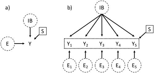
Figure 3a is similar to Figure 6c in Deffner et al. (2022). However, they showed a latent variable with only one observed variable, which is not very common in psychological (questionnaire) assessment. In Figure 3b, the complete measurement model of IB is shown with a selection node pointing into potentially all observed variables $Y_{1-5}.$ If one can make more detailed assumptions about group-specific selection mechanisms on the observed variables, the selection node could also only point into some, but not all, of the items. In the psychometric literature, this is often referred to as differential item functioning (Holland & Wainer, 2012; Zumbo, 2007). As Deffner and colleagues state, Figure 3 shows a selection node pointing into an outcome. This prevents unbiased comparisons of the observed (and consequently, the latent) variables between groups. Similar to what we mentioned in the introduction, an absent selection node is a stronger assumption than an existent one. Not drawing a selection node pointing into an observed variable encodes the assumption that this variable (here: questionnaire item) is invariant across all groups. In Figure 3, the selection node pointing into Y could subsume all four levels of non-invariance. By translating the DAG with a selection node (also called selection diagram) into a path diagram, we can see that one DAG implies many different models. In Figure 4, four different pairs (each consisting of group western and group eastern) of models are shown, where each pair depicts one level of MI being violated. The group-specific distribution of Y could stem from:

Figure 4. Pairs of measurement models of IB (impartial beneficence) for which measurement invariance does not hold between the two groups. (a) violation of configural invariance (violation of configural invariance due to different number of latent variables between groups is not displayed); (b) violation of metric invariance (assuming standardized data); (c) violation of scalar invariance; (d) violation of residual invariance (assuming unstandardized data). Parameters that differ between groups are highlighted in blue.

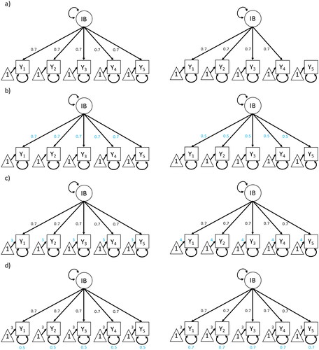
1. some paths between IB and Y being 0 in one group or a different number of latent variables between groups (configural non-invariance; Figure 4a),

2. the size of the loadings $\lambda$ between IB and Y being different between groups (metric; Figure 4b),

3. the intercepts $\tau$ of Y being different between groups (scalar; Figure 4c),

4. or the variances of the unique errors E of Y being different between groups (residual; Figure 4d).

Now that we have introduced how to depict non-invariance with a selection diagram,⁵ we can turn to a more elaborate example. Specifically, we now demonstrate how DAGs can be used to make informed modeling decisions when investigating MI. We show how disregarding the complete causal model and instead only considering the groups that we want to compare, can miss important aspects of non-invariance. All code needed to reproduce the results of the following simulated and empirical example as well as a reproducible manuscript are available at https://osf.io/2mpq9/.

All analyses were conducted in the statistical software R (R Core Team, 2021), using the packages lavaan (Rosseel, 2012), semTools (Jorgensen et al., 2016), and OpenMx (Boker et al., 2011). The paper was written using the package papaja (Aust & Barth, 2020).

4. A More Holistic View on Measurement Invariance

We again consider our example in Figure 3b), that is, we want to compare the latent means of IB between groups western and eastern (defined by the covariate Region). To investigate whether scores of IB are comparable between these two groups, that is, if the measurement models are equivalent, we would first conduct a MG-CFA with Region as the grouping covariate. However, assume that the true data-generating process is not the one in Figure 3b) but the one in Figure 5, where an observed covariate Age is part of the measurement model.

Figure 5. DAG with a selection node pointing into the observed covariate Age which influences all observed variables $Y_{1-5}$ (depicted by the dotted box around the observed variables).

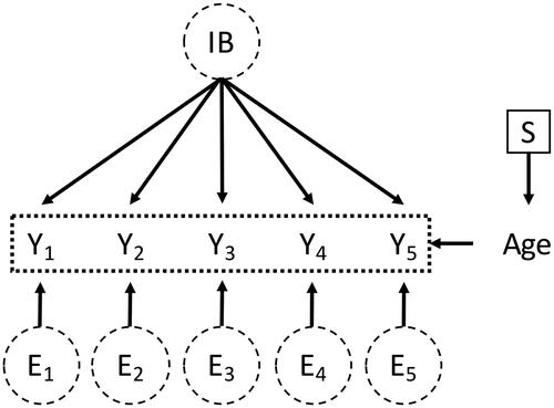
In this setting, the selection node actually points into Age, not into the items $Y_{1-5}.$ This means that not the distribution of $Y_{1-5}$ varies between groups but the distribution of Age. Specifically, in group 1, $\mathit{\text{Age}}\sim N(0,1)$ and in group 2, $\mathit{\text{Age}}\sim N(0.5,1)$ (standardized ages where the mean age is higher in group 2 than in group 1). In this case, assume $\mathit{\text{IB}}\to Y\leftarrow \mathit{\text{Age}}$ to be an interaction between IB and Age, such that the measurement model for every item is $Y=(\sqrt{0.6}+0.3\mathit{\text{Age}})·\mathit{\text{IB}}+E$ (cf. Equation (1)(1) $$\mathit{Y}=\mathit{\tau }+\mathbf{\Lambda }C+\mathit{E}$$(1) ).⁶ That is, with increasing Age, the causal relationship between the latent variable IB and the observed variables $Y_{1-5}$ grows stronger.

A small simulation of the model depicted in Figure 5⁷ reveals the following: If we do not consider the DAG in Figure 5 and test MI following the current practice, that is, only test the invariance of measurement models between groups western and eastern, we find a significant violation of metric MI (${\chi }^2(14;N=1,000)=19.46,$ $p=.003$ and an increase in RMSEA of .028 for the comparison of the configural and the metric model). However, this result is only half of the picture: It is the different distribution of Age between groups that is decisive for the result of the MI test. That is, the group-specific mechanism, indicated by the selection node, is working on Age, not on the observed variables directly. Conclusions regarding different interpretations of the construct between groups western and eastern based on the MI test results are rather uninformative.

How could DAGs have helped us to achieve more informative results regarding MI? Had we set up the selection diagram (by theoretical or empirical considerations) as in Figure 5, we would have seen that MG-CFA with Region as a grouping covariate is not the right model. Instead, we have to resort to a more flexible model to investigate MI in this case. We can read from the DAG that Age is an assumed direct cause of $Y_{1-5}$ and that we assume Age to have a group-specific distribution. Thus, we want to include Age in our model in order to close the path between the selection node and the observed variables $Y_{1-5}$ (remember that including Age in the model closes the path $\boxed{S}\to \mathit{\text{Age}}\to Y$). Generally speaking, our goal is to make as many assumptions as possible about covariates between the outcome (in our case Y) and the selection node, and then include these covariates in the model. This lets us gain more detailed information about group-specific mechanisms (i.e., non-invariance) in the data-generating process and how these mechanisms influence our observed variables.

One option to model the data-generating process depicted in Figure 5 is a type of moderated SEM called moderated non-linear factor analysis (MNLFA) (Bauer, 2017; Bauer & Hussong, 2009). MNLFA is especially suitable in this case because it allows the model parameters to depend on any covariate V in the data. In our example, we can model the expected loadings and intercepts by the regression equations ${\mathbf{\Lambda }}_i={\mathbf{\Lambda }}_0+{\mathit{D}}_{\mathit{\text{Region}}}{\mathit{\text{Region}}}_i+{\mathit{D}}_{\mathit{\text{Age}}}{\mathit{\text{Age}}}_i$ and ${\mathit{\tau }}_i={\mathit{\tau }}_0+{\mathit{b}}_{\mathit{\text{Region}}}{\mathit{\text{Region}}}_i+{\mathit{b}}_{\mathit{\text{Age}}}{\mathit{\text{Age}}}_i,$ respectively.⁸ ${\mathbf{\Lambda }}_0$ and ${\mathit{\tau }}_0$ are the baseline loadings and intercepts, $\mathit{D}$ and $\mathit{b}$ are vectors⁹ of linear effects of the covariates Region and Age on the parameters, and i denotes the person index. This model formulation allows us to estimate the baseline parameters as well as the individual effects a covariate has on the item parameters. Of course, if more detailed assumptions about which items are influenced by the covariates can be made, the equations above can be adjusted by setting the effects of the covariates on some items to 0. The covariate Region is also included to test its direct effect on the parameters (besides the assumed direct causal effect of Age). MNLFA can be estimated in R (R Core Team, 2021) via the package OpenMx (Boker et al., 2011). We refer readers to Kolbe et al. (2022) for a detailed guide on how to estimate MNLFA in OpenMx and specifically how to use it to investigate MI.

From a causal inference perspective, we can justify the model choice like this: the less we know about our measurement model and the covariates surrounding it, the more potential differences in parameters we have to consider during estimation and testing. The more potential differences we have to consider, the more arrows we should draw in our DAG.

5. Simulated Example

Table 1 shows the estimated results of a MNLFA for the simulated example described above. The model parameters (in our example: loadings and intercepts) are allowed to be moderated by covariates Region and Age as described above. This is the configural model. The advantage of modeling the assumed causal relationships like this is that we get detailed estimates of parameters and possible interactions for every item. As can be seen, Region does not have an influence on neither intercepts nor loadings, whereas Age has an influence of around 0.3 on the baseline loadings ${\mathbf{\Lambda }}_0,$ which are around $\sqrt{0.6}.$ Beyond visual inspection of the parameter estimates, we can also investigate metric and scalar MI. This is done by setting the effects of the covariates on the loadings (for metric MI), and loadings as well as intercepts (for scalar MI) to 0 and comparing these nested models. The results of this model comparison are shown in Table 2. They show that metric MI is violated (by the covariate Age), whereas scalar MI is supported (i.e., there is no significant moderation of the intercepts by the covariates).

Table 1. Results of moderated non-linear factor analysis for the toy example.

Item	${\tau }_0$	$b_{\mathit{\text{Region}}}$	$b_{\mathit{\text{Age}}}$	${\Lambda }_0$	$D_{\mathit{\text{Region}}}$	$D_{\mathit{\text{Age}}}$
Item 1	−0.07	0.15	−0.05	1.04	−0.05	0.00
Item 2	−0.08	0.03	−0.03	0.80	−0.07	0.35
Item 3	−0.06	0.12	−0.04	0.75	0.01	0.27
Item 4	−0.09	0.06	−0.04	0.74	−0.03	0.30
Item 5	−0.04	0.04	−0.05	0.73	0.04	0.30

Note. ${\tau }_0$ = Baseline intercepts, $b_{\mathit{\text{Region}}}$ = (Additive) Effects of covariate Region on baseline intercepts, $b_{\mathit{\text{Age}}}$ = (Linear) Effects of covariate Age on baseline intercepts, ${\Lambda }_0$ = Baseline loadings, $D_{\mathit{\text{Region}}}$ = (Additive) Effects of covariate Region on baseline loadings, $D_{\mathit{\text{Age}}}$ = (Linear) Effects of covariate Age on baseline loadings. Effects of Region and Age on other model parameters, e.g., residual variances, are not reported here. Reference category of Region is Eastern. The loading of item 1 was simulated as 1 for identification purposes.

Table 2. Results of ${\chi }^2$-difference tests between the configural, metric, and scalar moderated non-linear factor analyses for the simulated example.

Comparison	$\Delta -2\mathit{\text{LL}}$	$\Delta \mathit{\text{df}}$	p-Value
Configural vs. metric	290.39	10.00	0.00
Metric vs. scalar	−113.63	6.00	1.00

Note. $\Delta -2\mathit{\text{LL}}$ = difference in −2 times the log-likelihood of the models, $\Delta \mathit{\text{df}}$ = Difference in degrees of freedom. A p-value of 0 means that it is $<0.005.$

By taking into account the whole causal model and using a more flexible method than simply relying on MG-CFA, we can make a more informed decision regarding MI. Had we only used MG-CFA, we would try to explain why the two regions western and eastern have non-invariant measurement models, which would be the wrong question. On the basis of theoretical and empirical assumptions regarding the causal relationships, however, we can now reason about why the relationship between the latent variable IB and its items grows stronger with increasing age. It should be highlighted again that drawing a DAG with many arrows and using MNLFA entails less assumptions (or assumptions that are less strong) than using MG-CFA with one covariate. From a causal inference perspective, MG-CFA could be seen as the MI testing approach with the most assumptions.

6. Empirical Example

To mimic the analysis of the simulated example in the example on the real data published by Bago et al. (2022), we only considered observations from group western whose age was above 30 years. This was done to achieve two approximately equally sized groups ($n_{\mathit{\text{western}}}=2,911;$ $n_{\mathit{\text{eastern}}}=2,941$) with differing mean ages ($M_{\mathit{\text{western}}}=43.22;$ $M_{\mathit{\text{eastern}}}=26.13$). Note that this changes the real data, which was done simply for didactic purposes; the following results should not be interpreted from a substantive research perspective.

Table 3 shows the results of a MG-CFA, where again a one-dimensional model is specified and MI is investigated between the two groups western and eastern. We see that the results of the ${\chi }^2$-difference test is statistically significant for the evaluation of both metric and scalar MI. This is an indication that neither of these two levels of MI hold, that is, neither loadings nor intercepts are equivalent across groups. Considering the RMSEA, the difference between the configural and metric model does not exceed commonly suggested cut-offs, therefore supporting metric MI (Chen, 2007; Cheung & Rensvold, 2002; Rutkowski & Svetina, 2014). The RMSEA difference between the metric and the scalar model again indicates a violation of scalar MI. Based on these results, all we can conclude for now is that MI does not hold between the two regions western and eastern.

Table 3. Results of multi-group confirmatory factor analysis for the empirical example between regions Western and Eastern.

Model	df	${\chi }^2$	$\Delta {\chi }^2$	$\Delta \mathit{\text{df}}$	p-Value	RMSEA
Configural	10	104.36	–	–	–	0.06
Metric	14	142.72	38.36	4	0.00	0.06
Scalar	18	373.54	230.83	4	0.00	0.08

Note. df = Degrees of freedom, ${\chi }^2$ = Value of the test statistic, $\Delta {\chi }^2$ = Difference in values of the test statistics, $\Delta \mathit{\text{df}}$ = Difference in degrees of freedom, RMSEA = Root mean square error of approximation. A p-value of 0 means that it is $<0.005.$

To be able to reason more about the role of non-invariance in the underlying data-generating process, we again have to consider the complete DAG and model the data-generating process accordingly. Table 4 shows the results of a MNLFA, where both covariates Age and Region are allowed to moderate the parameter estimates. In the empirical example, these results paint a different picture than before. Age has no effect on both loadings and intercepts, whereas Region directly influences (primarily) the item intercepts. Specifically, in the group western, the intercepts of items 1, 2, and 4 are higher compared to group eastern, whereas for item 3, the intercept is lower. Effects of Region on the loadings are less strong. Similar to the simulated example, a ${\chi }^2$-difference test can be conducted. By this we can test whether allowing that the parameters are moderated by the covariates Region and Age significantly increases model fit (and thus, whether MI is violated).

Table 4. Results of moderated non-linear factor analysis for the empirical example.

Item	${\tau }_0$	$b_{\mathit{\text{Region}}}$	$b_{\mathit{\text{Age}}}$	${\Lambda }_0$	$D_{\mathit{\text{Region}}}$	$D_{\mathit{\text{Age}}}$
Item 1	3.68	0.22	0.00	0.96	−0.16	0.00
Item 2	3.21	0.24	0.01	1.41	0.02	−0.01
Item 3	4.26	−0.19	0.01	0.68	0.12	0.00
Item 4	2.77	0.49	0.02	0.82	0.10	0.00
Item 5	3.42	0.05	0.01	1.17	−0.10	0.00

Note. ${\tau }_0$ = Baseline intercepts, $b_{\mathit{\text{Region}}}$ = (Additive) Effects of covariate Region on baseline intercepts, $b_{\mathit{\text{Age}}}$ = (Linear) Effects of covariate Age on baseline intercepts, ${\Lambda }_0$ = Baseline loadings, $D_{\mathit{\text{Region}}}$ = (Additive) Effects of covariate Region on baseline loadings, $D_{\mathit{\text{Age}}}$ = (Linear) Effects of covariate Age on baseline loadings. Effects of Region and Age on other model parameters, e.g., residual variances, are not reported here. Reference category of Region is Eastern.

Table 5 shows that both levels of MI, metric and scalar, are violated. That is, the covarirates Region and Age significantly influence the loadings and intercepts in our measurement model. Because the model outputs estimates for all item parameters and their moderators, we are able to reason in more detail about the causes of non-invariance, given our assumptions encoded in the DAG. Of course, detailed inspection of item contents would now be necessary to explain why a covariate influences the item parameters. Since this would be beyond the scope of this paper and since we are not subject matter experts in moral psychology, we end our empirical demonstration here. However, we hope that this example proves as a starting point for showing how MI can be investigated according to the underlying causal assumptions.

Table 5. Results of ${\chi }^2$-difference tests between the configural, metric, and scalar moderated non-linear factor analyses for the empirical example.

Comparison	$\Delta -2\mathit{\text{LL}}$	$\Delta \mathit{\text{df}}$	p-Value
Configural vs. metric	44.66	10.00	0.00
Metric vs. scalar	276.26	6.00	0.00

Note. $\Delta -2\mathit{\text{LL}}$ = difference in –2 times the log-likelihood of the models, $\Delta \mathit{\text{df}}$ = Difference in degrees of freedom. A p-value of 0 means that it is $<0.005.$

7. Discussion

In this paper, we first introduced the connection between DAGs used in causal inference and path diagrams of measurement models, which are more common in the psychometric literature. We then showed how a lack of MI can be depicted by a DAG. We demonstrated how taking into account the causal relationships between the measurement model and the surrounding covariates yields more informative results when investigating MI. If MI is directly violated by a covariate that is not of primary interest (e.g., age in our example above), DAGs can help to visualize the underlying assumptions. Specifically, they depict the assumed mechanisms by which the data-generating process differs between groups. In this, researchers can find appropriate statistical models like MNLFA that allow them to estimate an extended measurement model. This also lets us reason about the causes of non-invariance. Only by investigating why MI does not hold, we can see it as an important finding by itself and draw conclusions about how different groups interpret a construct (Putnick & Bornstein, 2016).

One critique against DAGs is that it is difficult to specify all causal relationships (surrounding the measurement model, in our case). This is true but we deem this an argument against poor psychological theories and not against DAGs. A sound theory should allow us to specify the relationships between the variables it comprises. Besides, as mentioned in the introduction, also an incomplete or even wrong DAG can help us to reveal specific issues in theories. For example, drawing a DAG and realizing that there is uncertainty regarding some relationships, can be the starting point of further scientific discourse. In the end, DAGs are not about adding assumptions—they are about revealing the assumptions that are otherwise made implicitly (Deffner et al., 2022; Pearl & Bareinboim, 2014).

DAGs and path diagrams are part of a broader class of graphical models that have been introduced in the psychometric literature. Other examples are graphical Rasch models and graphical regression models that explicitly depict and model differential item functioning or local dependence (i.e., correlated item responses even after conditioning on the latent variable) (Anderson & Böckenholt, 2000; Kreiner & Christensen, 2002, 2011). Similarly, latent class models have been visualized as categorical causal models, again facilitating the representation of underlying model assumptions, such as local independence (Bartolucci & Forcina, 2005; Hagenaars, 1998; Humphreys & Titterington, 2003; Rijmen et al., 2008). In this notion, local dependence is intertwined with unobserved confounding (i.e., failing to include a covariate that influences the item response in the measurement model).

8. Limitations and Future Research

Our goal was to provide a translation between path diagrams of measurement models and DAGs, thereby framing MI and its investigation as a causal inference problem. In this, we showed only one example with one observed covariate (i.e., age with different distributions between groups). Needless to say, many more causal relationships leading to a violation of MI are conceivable, for example one in which the cause of non-invariance is latent. A prominent example of this in the literature is acquiescence bias, that is, the tendency of respondents to agree more to statements or items, irrespective of the content of the item (D’Urso et al., 2023; Lechner et al., 2019). Even further, beyond the representation of latent variables as common causes of observed variables, DAGs might help to depict (non-)invariance in other representations of multivariate data. Most notably, network models have been proposed as such an alternative conceptualization (Borsboom et al., 2021), and this field is increasingly interested in the investigation of invariance of networks across groups (e.g., Hoekstra et al., 2023). In these cases, graphical tools from the causal inference literature might also aid to reason about the causes of non-invariance and to find appropriate approaches with which the causal relationships can be modeled. Future studies could therefore illustrate the usefulness of DAGs when investigating MI in different scenarios or conceptualizations.

9. Conclusion

Many psychological studies concern some comparison of latent scores between groups. Investigating whether measurement models of the latent variables are equivalent between groups is crucial for unbiased conclusions. We discussed a theoretical framework in which MI can be viewed from a causal inference perspective. Reasoning about causes of differences in how constructs and their measures function across groups can create valuable insights for scale construction or even theory building. Drawing a DAG which encodes assumptions about non-invariance helps researchers to make informed modeling choices. In this, it might encourage them to view MI as part of the modeling process and as an interesting topic of research by itself—and not just as an additional test prior to the actual data analysis. Ultimately, we hope to contribute to an increase in the prevalence of investigations of MI.

Authors Contributions

The authors made the following contributions. Philipp Sterner: Conceptualization, Methodology, Formal Analysis, Visualization, Writing—Original Draft Preparation, Writing—Review and Editing; Florian Pargent: Conceptualization, Methodology, Writing—Review and Editing; Dominik Deffner: Methodology, Writing—Review and Editing; David Goretzko: Conceptualization, Methodology, Writing—Review and Editing, Supervision.

Notes

1 Double-headed arrows are sometimes used in DAGs to depict an unobserved common cause between two variables (Elwert, 2013). However, a double-headed arrow between A and B is identical to $A\leftarrow U\to B,$ where U is the unobserved common cause of both A and B. We restrict ourselves to the use of single-headed arrows in this paper.

2 Without loss of generality, we are assuming a one-dimensional construct (only one common factor C) and drop the person-indeces i for better readability.

3 In path diagrams, double-headed arrows between observed variables (i.e., items) are sometimes used to depict correlated error terms (i.e., item responses that are correlated even after conditioning on the latent variable). This is closely related to the double-headed arrows in DAGs mentioned in an earlier footnote. Correlated errors are equivalent to unobserved confounding, that is, failure to model all influence on the item response besides the latent variable. In the literature on item response models, this is often called local dependence (Kreiner & Christensen, 2011).

4 But see Bollen and Pearl (2013) who briefly touch on measurement models in combination with causality.

5 The use of selection nodes to depict non-invariance highlights that—from a causal inference perspective—the concept of MI is related to transportability. We refer interested readers to Deffner et al. (2022) and Pearl and Bareinboim (2014) for more details.

6 Because DAGs do not impose a functional form on the relationships between variables, all variables jointly causing another variable can also interact (Deffner et al., 2022; Elwert, 2013).

7 With $N=1000$ ($n=500$ per group), $\mathit{\text{IB}}\sim N(0,1),$ and $\mathit{\text{diag}}(\Psi )\sim \mathit{\text{Uniform}}(0.2,0.6).$ Together with loadings of $\sqrt{0.6},$ this results in an average item variance of 1.

8 Similarly, all other model parameters—like factor means or residual covariances—can be modeled as functions of covariates. Thus, MNLFA could be seen as a flexible extension to multiple indicator multiple cause models (MIMIC models; Muthén, 1989).

9 In case of more than one latent variable, $\mathit{D}$ would be a matrix with the same dimensions as ${\mathbf{\Lambda }}_0.$

References

- Anderson, C. J., & Böckenholt, U. (2000). Graphical regression models for polytomous variables. Psychometrika, 65, 497–509. https://doi.org/10.1007/BF02296340
- Asparouhov, T., & Muthén, B. O. (2014). Multiple-group factor analysis alignment. Structural Equation Modeling, 21, 495–508. https://doi.org/10.1080/10705511.2014.919210
- Aust, F., & Barth, M. (2020). Papaja: Create APA manuscripts with R Markdown. https://github.com/crsh/papaja
- Bago, B., Kovacs, M., Protzko, J., Nagy, T., Kekecs, Z., Palfi, B., Adamkovic, M., Adamus, S., Albalooshi, S., Albayrak-Aydemir, N., Alfian, I. N., Alper, S., Alvarez-Solas, S., Alves, S. G., Amaya, S., Andresen, P. K., Anjum, G., Ansari, D., Arriaga, P., … Aczel, B. (2022). Situational factors shape moral judgements in the trolley dilemma in Eastern, Southern and Western countries in a culturally diverse sample. Nature Human Behaviour, 6, 880–895. https://doi.org/10.1038/s41562-022-01319-5
- Bartolucci, F., & Forcina, A. (2005). Likelihood inference on the underlying structure of IRT models. Psychometrika, 70, 31–43. https://doi.org/10.1007/s11336-001-0934-z
- Bastian, B., Kuppens, P., De Roover, K., & Diener, E. (2014). Is valuing positive emotion associated with life satisfaction? Emotion, 14, 639–645. https://doi.org/10.1037/a0036466
- Bauer, D. J. (2017). A more general model for testing measurement invariance and differential item functioning. Psychological Methods, 22, 507–526. https://doi.org/10.1037/met0000077
- Bauer, D. J., Belzak, W. C. M., & Cole, V. T. (2020). Simplifying the assessment of measurement invariance over multiple background variables: Using regularized moderated nonlinear factor analysis to detect differential item functioning. Structural Equation Modeling, 27, 43–55. https://doi.org/10.1080/10705511.2019.1642754
- Bauer, D. J., & Hussong, A. M. (2009). Psychometric approaches for developing commensurate measures across independent studies: Traditional and new models. Psychological Methods, 14, 101–125. https://doi.org/10.1037/a0015583
- Belzak, W. C. M., & Bauer, D. J. (2020). Improving the assessment of measurement invariance: Using regularization to select anchor items and identify differential item functioning. Psychological Methods, 25, 673–690. https://doi.org/10.1037/met0000253
- Boker, S., Neale, M., Maes, H., Wilde, M., Spiegel, M., Brick, T., Spies, J., Estabrook, R., Kenny, S., Bates, T., Mehta, P., & Fox, J. (2011). OpenMx: An open source extended structural equation modeling framework. Psychometrika, 76, 306–317. https://doi.org/10.1007/s11336-010-9200-6
- Bollen, K. A. (1989). Structural equations with latent variables. John Wiley & Sons.
- Bollen, K. A., & Pearl, J. (2013). Eight myths about causality and structural equation models. In S. L. Morgan (Ed.), Handbook of causal analysis for social research (pp. 301–328). Springer Netherlands. https://doi.org/10.1007/978-94-007-6094-3_15
- Borsboom, D. (2023). Psychological constructs as organizing principles. In L. A. van der Ark, W. H. M. Emons, & R. R. Meijer (Eds.), Essays on contemporary psychometrics (pp. 89–108). Springer International Publishing. https://doi.org/10.1007/978-3-031-10370-4_5
- Borsboom, D., Deserno, M. K., Rhemtulla, M., Epskamp, S., Fried, E. I., McNally, R. J., Robinaugh, D. J., Perugini, M., Dalege, J., Costantini, G., Isvoranu, A.-M., Wysocki, A. C., Borkulo, C. D., Van, Van Bork, R., & Waldorp, L. J. (2021). Network analysis of multivariate data in psychological science. Nature Reviews Methods Primers, 1, 1–18. https://doi.org/10.1038/s43586-021-00055-w
- Brandmaier, A. M., Oertzen, T. v., McArdle, J. J., & Lindenberger, U. (2013). Structural equation model trees. Psychological Methods, 18, 71–86. https://doi.org/10.1037/a0030001
- Chen, F. F. (2007). Sensitivity of goodness of fit indexes to lack of measurement invariance. Structural Equation Modeling, 14, 464–504. https://doi.org/10.1080/10705510701301834
- Cheung, G. W., & Rensvold, R. B. (2002). Evaluating goodness-of-fit indexes for testing measurement invariance. Structural Equation Modeling, 9, 233–255. https://doi.org/10.1207/S15328007SEM0902_5
- D’Urso, E. D., Tijmstra, J., Vermunt, J. K., & De Roover, K. (2023). Does acquiescence disagree with measurement invariance testing? Structural Equation Modeling, 0, 1–15. https://doi.org/10.1080/10705511.2023.2260106
- De Roover, K., Vermunt, J. K., & Ceulemans, E. (2022). Mixture multigroup factor analysis for unraveling factor loading noninvariance across many groups. Psychological Methods, 27, 281–306. https://doi.org/10.1037/met0000355
- Deffner, D., Rohrer, J. M., & McElreath, R. (2022). A causal framework for cross-cultural generalizability. Advances in Methods and Practices in Psychological Science, 5. https://doi.org/10.1177/25152459221106366
- Elwert, F. (2013). Graphical causal models. In S. L. Morgan (Ed.), Handbook of causal analysis for social research (pp. 245–273). Springer Netherlands. https://doi.org/10.1007/978-94-007-6094-3_13
- Epskamp, S. (2015). semPlot: Unified visualizations of structural equation models. Structural Equation Modeling, 22, 474–483. https://doi.org/10.1080/10705511.2014.937847
- Goretzko, D., Siemund, K., & Sterner, P. (2023). Evaluating model fit of measurement models in confirmatory factor analysis. Educational and Psychological Measurement, 84, 123–144. https://doi.org/10.1177/00131644231163813
- Greenland, S., & Brumback, B. (2002). An overview of relations among causal modelling methods. International Journal of Epidemiology, 31, 1030–1037. https://doi.org/10.1093/ije/31.5.1030
- Hagenaars, J. A. (1998). Categorical causal modeling: Latent class analysis and directed log-linear models with latent variables. Sociological Methods & Research, 26, 436–486. https://doi.org/10.1177/0049124198026004002
- Hoekstra, R. H. A., Epskamp, S., Nierenberg, A., Borsboom, D., & McNally, R. J. (2023). Testing similarity in longitudinal networks. The Individual Network Invariance Test. https://doi.org/10.31234/osf.io/ugs2r
- Holland, P. W., & Wainer, H. (2012). Differential item functioning. Routledge.
- House, B. R., Kanngiesser, P., Barrett, H. C., Broesch, T., Cebioglu, S., Crittenden, A. N., Erut, A., Lew-Levy, S., Sebastian-Enesco, C., Smith, A. M., Yilmaz, S., & Silk, J. B. (2020). Universal norm psychology leads to societal diversity in prosocial behaviour and development. Nature Human Behaviour, 4, 36–44. https://doi.org/10.1038/s41562-019-0734-z
- Humphreys, K., & Titterington, D. M. (2003). Variational approximations for categorical causal modeling with latent variables. Psychometrika, 68, 391–412. https://doi.org/10.1007/BF02294734
- Jöreskog, K. G. (1967). Some contributions to maximum likelihood factor analysis. Psychometrika, 32, 443–482. https://doi.org/10.1007/BF02289658
- Jöreskog, K. G. (1971). Simultaneous factor analysis in several populations. Psychometrika, 36, 409–426. https://doi.org/10.1007/BF02291366
- Jorgensen, T. D., Pornprasertmanit, S., Schoemann, A. M., Rosseel, Y., Miller, P., Quick, C., Garnier-Villarreal, M., Selig, J., Boulton, A., Preacher, K., et al. (2016). Package “semtools.” https://cran.r-project.org/web/packages/semtools/semtools.pdf.
- Kahane, G., Everett, J. A. C., Earp, B. D., Caviola, L., Faber, N. S., Crockett, M. J., & Savulescu, J. (2018). Beyond sacrificial harm: A two-dimensional model of utilitarian psychology. Psychological Review, 125, 131–164. https://doi.org/10.1037/rev0000093
- Kim, E., Cao, C., Wang, Y., & Nguyen, D. (2017). Measurement invariance testing with many groups: A comparison of five approaches. Structural Equation Modeling, 24, 524–544. https://doi.org/10.1080/10705511.2017.1304822
- Kolbe, L., Molenaar, D., Jak, S., & Jorgensen, T. D. (2022). Assessing measurement invariance with moderated nonlinear factor analysis using the R package OpenMx. Psychological Methods, https://doi.org/10.1037/met0000501
- Kopf, J., Zeileis, A., & Strobl, C. (2015). Anchor selection strategies for DIF analysis: Review, assessment, and new approaches. Educational and Psychological Measurement, 75, 22–56. https://doi.org/10.1177/0013164414529792
- Kreiner, S., & Christensen, K. B. (2002). Graphical Rasch models. In M. Mesbah, B. F. Cole, & M.-L. T. Lee (Eds.), Statistical methods for quality of life studies: Design, measurements and analysis (pp. 187–203). Springer US. https://doi.org/10.1007/978-1-4757-3625-0_15
- Kreiner, S., & Christensen, K. B. (2011). Item screening in graphical Loglinear Rasch models. Psychometrika, 76, 228–256. https://doi.org/10.1007/s11336-011-9203-y
- Kunicki, Z. J., Smith, M. L., & Murray, E. J. (2023). A primer on structural equation model diagrams and directed acyclic graphs: When and how to use each in psychological and epidemiological research. Advances in Methods and Practices in Psychological Science, 6. https://doi.org/10.1177/25152459231156085
- Lechner, C. M., Partsch, M. V., Danner, D., & Rammstedt, B. (2019). Individual, situational, and cultural correlates of acquiescent responding: Towards a unified conceptual framework. The British Journal of Mathematical and Statistical Psychology, 72, 426–446. https://doi.org/10.1111/bmsp.12164
- Leitgöb, H., Seddig, D., Asparouhov, T., Behr, D., Davidov, E., De Roover, K., Jak, S., Meitinger, K., Menold, N., Muthén, B. O., Rudnev, M., Schmidt, P., & Schoot, R. v d (2023). Measurement invariance in the social sciences: Historical development, methodological challenges, state of the art, and future perspectives. Social Science Research, 110, 102805. https://doi.org/10.1016/j.ssresearch.2022.102805
- Lord, F. M., & Novick, M. R. (1968). Statistical theories of mental test scores. IAP.
- Luong, R., & Flake, J. K. (2023). Measurement invariance testing using confirmatory factor analysis and alignment optimization: A tutorial for transparent analysis planning and reporting. Psychological Methods, 28, 905–924. https://doi.org/10.1037/met0000441
- Maassen, E., D'Urso, E. D., van Assen, M. A. L. M., Nuijten, M. B., De Roover, K., & Wicherts, J. M. (2023). The dire disregard of measurement invariance testing in psychological science. Psychological Methods. https://doi.org/10.1037/met0000624
- Mellenbergh, G. J. (1989). Item bias and item response theory. International Journal of Educational Research, 13, 127–143. https://doi.org/10.1016/0883-0355(89)90002-5
- Meredith, W. (1993). Measurement invariance, factor analysis and factorial invariance. Psychometrika, 58, 525–543. https://doi.org/10.1007/BF02294825
- Meuleman, B., Żółtak, T., Pokropek, A., Davidov, E., Muthén, B., Oberski, D. L., Billiet, J., & Schmidt, P. (2022). Why measurement invariance is important in comparative research. A response to Welzel et al. (2021). Sociological Methods & Research, 52, 1401–1419. https://doi.org/10.1177/00491241221091755
- Mulaik, S. A. (2009). Linear causal modeling with structural equations. CRC Press.
- Mulaik, S. A. (2010). Foundations of factor analysis. CRC press.
- Muthén, B. O. (1989). Latent variable modeling in heterogeneous populations. Psychometrika, 54, 557–585. https://doi.org/10.1007/BF02296397
- Pearl, J. (1988). Probabilistic reasoning in intelligent systems: Networks of plausible inference. Morgan Kaufmann.
- Pearl, J. (1998). Graphs, causality, and structural equation models. Sociological Methods & Research, 27, 226–284. https://doi.org/10.1177/0049124198027002004
- Pearl, J. (2012). The causal foundations of structural equation modeling. Defense Technical Information Center. https://doi.org/10.21236/ADA557445
- Pearl, J., & Bareinboim, E. (2014). External validity: From do-calculus to transportability across populations. Statistical Science, 29, 579–595. https://doi.org/10.1214/14-STS486
- Pohl, S., Schulze, D., & Stets, E. (2021). Partial measurement invariance: Extending and evaluating the cluster approach for identifying anchor items. Applied Psychological Measurement, 45, 477–493. https://doi.org/10.1177/01466216211042809
- Putnick, D. L., & Bornstein, M. H. (2016). Measurement invariance conventions and reporting: The state of the art and future directions for psychological research. Developmental Review, 41, 1–90. https://doi.org/10.1016/j.dr.2016.06.004
- Core Team, R. (2021). R: A language and environment for statistical computing. R Foundation for Statistical Computing. https://www.R-project.org/
- Rijmen, F., Vansteelandt, K., & De Boeck, P. (2008). Latent class models for diary method data: Parameter estimation by local computations. Psychometrika, 73, 167–182. https://doi.org/10.1007/s11336-007-9001-8
- Rohrer, J. M. (2018). Thinking Clearly about correlations and causation: graphical causal models for observational data. Advances in Methods and Practices in Psychological Science, 1, 27–42. https://doi.org/10.1177/2515245917745629
- Rosseel, Y. (2012). Lavaan: An R package for structural equation modeling. Journal of Statistical Software, 48, 1–36. https://doi.org/10.18637/jss.v048.i02
- Rudnev, M. (2019). Alignment method for measurement invariance: Tutorial. In Elements of cross-cultural research. https://maksimrudnev.com/2019/05/01/alignment-tutorial/
- Rutkowski, L., & Svetina, D. (2014). Assessing the hypothesis of measurement invariance in the context of large-scale international surveys. Educational and Psychological Measurement, 74, 31–57. https://doi.org/10.1177/0013164413498257
- Sass, D. A. (2011). Testing measurement invariance and comparing latent factor means within a confirmatory factor analysis framework. Journal of Psychoeducational Assessment, 29, 347–363. https://doi.org/10.1177/0734282911406661
- Schulze, D., & Pohl, S. (2021). Finding clusters of measurement invariant items for continuous covariates. Structural Equation Modeling, 28, 219–228. https://doi.org/10.1080/10705511.2020.1771186
- Seifert, I. S., Rohrer, J. M., & Schmukle, S. C. (2024). Using within-person change in three large panel studies to estimate personality age trajectories. Journal of Personality and Social Psychology, 126, 150–174. https://doi.org/10.1037/pspp0000482
- Steenkamp, J.-B. E. M., & Baumgartner, H. (1998). Assessing measurement invariance in cross-national consumer research. Journal of Consumer Research, 25, 78–107. https://doi.org/10.1086/209528
- Sterner, P., & Goretzko, D. (2023). Exploratory factor analysis trees: Evaluating measurement invariance between multiple covariates. Structural Equation Modeling, 30, 871–886. https://doi.org/10.1080/10705511.2023.2188573
- Strobl, C., Kopf, J., & Zeileis, A. (2015). Rasch trees: A new method for detecting differential item functioning in the Rasch model. Psychometrika, 80, 289–316. https://doi.org/10.1007/s11336-013-9388-3
- Suzuki, E., Shinozaki, T., & Yamamoto, E. (2020). Causal diagrams: Pitfalls and tips. Journal of Epidemiology, 30, 153–162. https://doi.org/10.2188/jea.JE20190192
- Tutz, G., & Schauberger, G. (2015). A penalty approach to differential item functioning in Rasch models. Psychometrika, 80, 21–43. https://doi.org/10.1007/s11336-013-9377-6
- Van Bork, R., Rhemtulla, M., Sijtsma, K., & Borsboom, D. (2022). A causal theory of error scores. Psychological Methods. https://doi.org/10.1037/met0000521
- Van De Schoot, R., Lugtig, P., & Hox, J. (2012). A checklist for testing measurement invariance. European Journal of Developmental Psychology, 9, 486–492. https://doi.org/10.1080/17405629.2012.686740
- Vandenberg, R. J., & Lance, C. E. (2000). A review and synthesis of the measurement invariance literature: Suggestions, practices, and recommendations for organizational research. Organizational Research Methods, 3, 4–70. https://doi.org/10.1177/109442810031002
- Westfall, J., & Yarkoni, T. (2016). Statistically controlling for confounding constructs is harder than you think. PloS One, 11, e0152719. https://doi.org/10.1371/journal.pone.0152719
- Wysocki, A. C., Lawson, K. M., & Rhemtulla, M. (2022). Statistical control requires causal justification. Advances in Methods and Practices in Psychological Science, 5. https://doi.org/10.1177/25152459221095823
- Zumbo, B. D. (2007). Three generations of DIF analyses: Considering where it has been, where it is now, and where it is going. Language Assessment Quarterly, 4, 223–233. https://doi.org/10.1080/15434300701375832