Predictable Losses of Liquidity Provision in Constant Function Markets and Concentrated Liquidity Markets

Abstract

We introduce a new comprehensive and model-free measure for the unhedgeable and predictable loss (PL) incurred by liquidity providers (LPs) in constant function markets (CFMs) and in concentrated liquidity markets. PL compares the value of the LP's holdings in the CFM liquidity pool (assuming no fee revenue) with that of a self-financing portfolio that (i) continuously replicates the dynamic holdings of the LP in the pool to offset the market risk of the LP's position, and (ii) invests in a risk-free account. We provide closed-form formulae for PL in CFMs with and without concentrated liquidity, and show that the losses stem from two sources: convexity cost, which depends on liquidity taking activity and the convexity of the pool's trading function; and opportunity cost, which is due to locking the LP's assets in the pool. For liquidity providers, PL is the appropriate measure to assess the cost of liquidity provision in CFMs, so that fees and compensation to LPs provide the right incentives for a well-functioning market. When prices form outside of the pool, we show that PL is reduced when liquidity taking is costly, i.e., when the convexity of the pool's trading function is high. On the other hand, when prices form in the pool, PL is reduced when liquidity taking is cheap, i.e., when the convexity of the trading function is low. Finally, we use Uniswap v3 and Binance transaction data to compute PL and fees collected by LPs and show that, at present, liquidity provision in CFMs is a loss-leading activity.

Keywords:

• Decentralised finance
• automated market making
• concentrated liquidity
• algorithmic trading
• predictable loss
• impermanent loss

1. Introduction

The emergence of decentralized finance (DeFi) ecosystems poses great challenges to traditional financial services based on intermediaries. Within DeFi, automated market makers (AMMs) are trading venues in which the rules to clear demand and supply depart considerably from those of the matching engines in traditional limit order books (LOBs). In contrast to traditional electronic exchanges which are organized around LOBs to clear demand and supply of liquidity, the takers and providers of liquidity in AMMs interact through liquidity pooling; liquidity providers (LPs) deposit their assets in a liquidity pool, and liquidity takers (LTs) exchange assets directly with the pool. Currently, the majority of AMMs are constant function markets (CFMs), and constant product markets (CPMs) with concentrated liquidity (CL) are the most popular type of CFM, with Uniswap v3 as a prime example; see Adams et al. (2021).

CFMs rely on a deterministic trading function and a set of rules to determine how liquidity takers and makers interact with the pool. In particular, the trading function determines marginal exchange rates (akin to the midprice in an LOB) and execution exchange rates (akin to the prices received by liquidity taking orders that walk the book) as a function of the quantity of the assets in the pool. We show that precluding roundtrip arbitrages where both legs are executed in the CFM requires a convex trading function.

A key difference between CFMs and LOBs is how liquidity is provided and compensated. In LOBs, market makers post liquidity on both sides of the midprice to earn the spread on roundtrip trades. In CFMs, LPs deposit their assets in the pool, and in CPMs with CL, LPs specify a range of exchange rates in which they deposit their assets. The assets rest in the pool until they are withdrawn and LPs are compensated with the fees paid by LTs who take liquidity from the pool. In current designs, the fees paid by LTs are a fixed percentage of the size of their liquidity taking trades. In CFMs, if LPs do not collect enough fees for making liquidity, their business is not viable because they would provide liquidity to the market at a loss.

In this paper, we focus on liquidity provision in CFMs and in CPMs with CL – see Cartea, Drissi and Monga (2022a) for an analysis of liquidity taking in these venues. For both types of venues, we derive the continuous-time dynamics of the wealth of LPs, and we introduce predictable loss (PL) which is a model-free measure that characterizes the inevitable and predictable losses of LPs. PL quantifies the loss of value when depositing one's assets in a CFM pool instead of holding a self-financing dynamic portfolio outside the pool that (i) replicates the risk of the LP's position in the pool and (ii) invests in a risk-free account. We prove that PL is a negative (i.e., LPs provide liquidity at a loss) and a predictable component in the dynamics of the LP position value in the pool. PL stems from two sources. One source is the convexity cost whose magnitude is a function of liquidity taking activity and the convexity of the CFM's trading function. The other source is the opportunity cost, which is incurred by LPs who lock assets in the pool instead of investing them in the risk-free asset.

Academics and practitioners commonly use impermanent loss (IL) to measure the losses incurred by LPs. IL quantifies the loss of value when depositing assets in a CFM pool instead of passively holding the assets outside the pool. We show that IL is not an appropriate measure because it can underestimate or overestimate the losses that are solely imputable to liquidity provision. In contrast, the convexity and opportunity costs of PL are predictable and unhedgeable components in the wealth of LPs. Moreover, we show that if the randomness in the marginal exchange rate of the CFM pool is exogenous (prices form outside the pool), then PL is reduced when the convexity of the trading function is high, i.e., when trading is costly. On the other hand, if the randomness in the marginal rate is a result of the liquidity taking trading activity (prices form in the pool), then PL is reduced when the convexity of the trading function is low, i.e., when trading is cheap.

Finally, we use Uniswap v3 data from the pool ETH/USDC (Ethereum and USD coin) between 5 May 2021 and 10 January 2023 to compute PL. Our analysis of the historical transactions in Uniswap v3 shows that the fees collected from market making activity are not enough to cover PL. To the best of our knowledge, this work is the first to (i) characterize the unhedgeable losses of LPs in closed-form in a model-free framework for CFMs, (ii) characterize the unhedgeable losses of LPs in closed-form in CPMs with CL, and (iii) derive the continuous-time dynamics for the wealth of LPs in CPMs with CL.

Previous works on AMMs are in Angeris et al. (2021), Chiu and Koeppl (2019), Lipton and Treccani (2021), Lipton and Hardjono (2021), and Lipton and Sepp (2021). Numerous works in the literature study liquidity provision in CFMs. Angeris and Chitra (2020) study but do not prove the convexity of the trading function, Cartea, Drissi and Monga (2022b) and Neuder et al. (2021) study strategic liquidity provision in CFMs with concentrated liquidity, and Fukasawa, Maire, and Wunsch (2023) study the hedging of the impermanent losses of LPs. Other works include Heimbach, Schertenleib, and Wattenhofer (2022) who discuss the tradeoff between risks and returns that LPs face in Uniswap v3, and Fan et al. (2022) who show how LPs can exploit their beliefs on future rates.

Another strand of the literature explores fee structures for fair compensation of LPs. Evans, Angeris, and Chitra (2021) study optimal fees in geometric markets, Sabate-Vidales and Šiška (2022) study variable fees in CPMs, and Cohen et al. (2023) derive a lower bound for fee revenue to make liquidity provision profitable in CFMs. Further, Cartea, Drissi and Monga (2022a), Cartea, Drissi, and Monga (2023), and Jaimungal et al. (2023) show how to optimally trade a large position and execute statistical arbitrages using signals in CPMs, Berg et al. (2022) empirically study inefficiencies in CFMs, and Bichuch and Feinstein (2022) introduce an axiomatic framework for CFMs and exchange rates. Finally, liquidity provision models in traditional markets are in Cartea, Jaimungal and Penalva (2015), Drissi (2022), Glosten and Milgrom (1985), Guéant, Lehalle, and Fernandez-Tapia (2012), and Guéant (2016).

The remainder of the paper proceeds as follows. Section 2 describes liquidity provision in CFMs and proves that a convex trading function does not admit instant roundtrip arbitrages. Next, we derive the wealth dynamics of LPs and introduce PL for CFMs as the combined effect of the convexity cost and the opportunity cost. Finally, we compare PL and IL for CFMs. Section 3.4 describes liquidity provision in CL pools. Next, we derive the continuous-time dynamics of the wealth of LPs, and we extend PL for passive and active LPs. Finally, Section 4 showcases PL in Uniswap v3 and shows that liquidity provision is not fairly compensated in the pool that we consider.

2. Predictable Losses of Liquidity Providers in CFMs

This section reviews how CFMs operate and discusses the profitability of liquidity provision measured with IL and PL. Subsection 2.1 recalls the LT and the LP provision conditions that determine how a CFM clears demand and supply. Subsection 2.2 first proves that roundtrip arbitrages within the CFM are not possible when the trading function is convex. Next, we introduce PL for CFMs as a comprehensive measure of the losses incurred by LPs and show that these losses result from (i) the convexity of the trading function and (ii) the opportunity cost from locking assets in the pool. Finally, Subsection 2.3 generalizes IL to CFMs and compares the measure with PL.

2.1. Constant Function Markets

Here, we recall the properties of CFMs; see Angeris and Chitra (2020); Angeris et al. (2021); Cartea, Drissi and Monga (2022a); Evans, Angeris, and Chitra (2021). Consider a risky asset Y that is valued in terms of a reference asset X and denote by Z the marginal exchange rate of asset Y in terms of asset X, where the rate Z is determined by the available liquidity in the pool. The marginal exchange rate of asset Y in terms of asset X is the exchange rate in the pool for a trade of infinitesimal size in asset Y . A CFM is characterized by a trading function $f:{\mathbb{R}}_{++}\times {\mathbb{R}}_{++}\mapsto \mathbb{R}$ which is continuously differentiable, convex, and increasing in its arguments; ${\mathbb{R}}_{++}$ denotes the set of positive real numbers. Below, we describe the LT trading condition and the LP provision condition for CFMs. These two conditions determine how market participants interact in the pool and how markets are cleared.

2.1.1. LT Trading Condition

Assume that the liquidity pool initially consists of quantity x of asset X and quantity y of asset Y . We refer to the pair $(x,y)$ as the reserves of the pool. LT transactions involve exchanging a quantity ${\mathrm{\Delta }}^y$ of asset Y for a quantity ${\mathrm{\Delta }}^x$ of asset X, and vice-versa. The quantities to exchange are determined by the LT trading function (1) $\begin{array}{r}f(x,y)=f(x+{\mathrm{\Delta }}^x,y-{\mathrm{\Delta }}^y)={\kappa }^2.\end{array}$(1) The value of the depth $\kappa >0$ is constant before and after a trade is executed, so the LT trading condition (1(1) $\begin{array}{r}f(x,y)=f(x+{\mathrm{\Delta }}^x,y-{\mathrm{\Delta }}^y)={\kappa }^2.\end{array}$(1) ) defines a level curve. For a fixed value of the depth κ, we define the level function ${\phi }_{\kappa }$ so that $f(x,y)={\kappa }^2⟺x={\phi }_{\kappa }\left(y\right)$¹. For any value κ of the depth, we assume that the level function ${\phi }_{\kappa }:{\mathbb{R}}_{++}\mapsto {\mathbb{R}}_{++}$ is twice differentiable.

The LT trading condition (1(1) $\begin{array}{r}f(x,y)=f(x+{\mathrm{\Delta }}^x,y-{\mathrm{\Delta }}^y)={\kappa }^2.\end{array}$(1) ) links the state of the pool before and after a liquidity taking trade is executed. For LTs, this condition specifies the exchange rate $\tilde{Z}\left({\mathrm{\Delta }}^y\right)=\left({\phi }_{\kappa }\right(y)-{\phi }_{\kappa }(y+{\mathrm{\Delta }}^y\left)\right)/{\mathrm{\Delta }}^y$ to trade a (possibly negative) quantity ${\mathrm{\Delta }}^y$ of asset Y , and the marginal exchange rate $Z=\underset{{\mathrm{\Delta }}^y\to 0}{lim}\tilde{Z}\left({\mathrm{\Delta }}^y\right)=-{\phi }_{\kappa }^{\mathrm{\prime }}\left(y\right)$ of asset Y in terms of asset X in the pool. In particular, Cartea, Drissi and Monga (2022a) show that one can use the convexity ${\phi }_{\kappa }^{\mathrm{\prime }\mathrm{\prime }}\left(y\right)$ of the level function to approximate the execution costs $|\tilde{Z}\left(\mathrm{\Delta }y\right)-Z|$ of LT trades in the pool. Below, we prove that there is no roundtrip arbitrage in a CFM if the level function φ is convex.

2.1.2. LP Provision Condition

Assume that the liquidity pool initially consists of quantity x of asset X and quantity y of asset Y . LP transactions involve depositing or withdrawing quantities $({\mathrm{\Delta }}^x,{\mathrm{\Delta }}^y)$ of asset X and asset Y . Let ${\kappa }_0$ be the initial depth of the pool and let ${\kappa }_1$ be the depth of the pool after an LP deposits $({\mathrm{\Delta }}^x,{\mathrm{\Delta }}^y)$, i.e., $f(x,y)={\kappa }_0^2$ and $f(x+\mathrm{\Delta }x,y+\mathrm{\Delta }y)={\kappa }_1^2$. Let ${\phi }_{{\kappa }_0}$ and ${\phi }_{{\kappa }_1}$ be the level functions corresponding to the values ${\kappa }_0$ and ${\kappa }_1$, respectively. Denote by Z the initial marginal exchange rate of the pool. The LP provision condition requires that LPs do not change the marginal rate Z, so (2) $\begin{array}{r}-{\phi }_{{\kappa }_0}^{\mathrm{\prime }}\left(y\right)=-{\phi }_{{\kappa }_1}^{\mathrm{\prime }}(y+{\mathrm{\Delta }}^y)=Z.\end{array}$(2) The LP provision condition (2(2) $\begin{array}{r}-{\phi }_{{\kappa }_0}^{\mathrm{\prime }}\left(y\right)=-{\phi }_{{\kappa }_1}^{\mathrm{\prime }}(y+{\mathrm{\Delta }}^y)=Z.\end{array}$(2) ) links the state of the pool before and after a liquidity provision operation is executed. The trading function $f(x,y)$ in (1(1) $\begin{array}{r}f(x,y)=f(x+{\mathrm{\Delta }}^x,y-{\mathrm{\Delta }}^y)={\kappa }^2.\end{array}$(1) ) is increasing in the pool quantities x and y. Thus, when liquidity provision activity increases (decreases) the size of the pool, the value of κ increases (decreases). For liquidity providers, the key difference between the traditional and the new venues is that in LOBs, market makers post limit orders above and below the midprice to earn the spread on roundtrip trades, while in CFMs, LPs earn fees paid by LTs when their liquidity is used. In LOBs, market makers are not present in the book after all their orders are either executed or canceled. On the other hand, in CFMs, posted liquidity remains in the pool until it is withdrawn by the LP. Indeed, in CFMs, LPs do not receive payments directly on their accounts and their holdings rest in the pool. Only when the LP removes her liquidity, are the accumulated fees paid into her account and any capital gains or losses are realized. In some CFMs, the fees are added to the stock of liquidity of LPs instead of accruing in separate accounts.

2.1.3. No Roundtrip Arbitrage and Convexity of the Level Function

There is roundtrip arbitrage if one can obtain a riskless profit from a buy/sell order immediately followed by a sell/buy order to close the position. This trade is profitable if and only if the ask/bid price is lower/greater than the bid/ask price. Proposition 2.1 shows that there are no roundtrip arbitrage opportunities in CFMs if the level function is convex.

Proposition 2.1

Let $\phi \in {\mathcal{C}}^2\left({\mathbb{R}}_{++}\right)$ be the level function of a CFM and assume there are no profitable instantaneous roundtrip arbitrages within the CFM. Then, φ is convex.

Proof.

Let $Z_t^{\text{bid}}\left({\mathrm{\Delta }}^y\right)$ and $Z_t^{\text{ask}}\left({\mathrm{\Delta }}^y\right)$ denote the exchange rates at time $t\in [0,T]$ obtained for a sell trade and a buy trade of size ${\mathrm{\Delta }}^y$, respectively. Assume there is no roundtrip arbitrage, so the bid-ask spread is nonnegative and we write (3) $\begin{array}{r}{Z}_t^{\text{bid}}\left({\mathrm{\Delta }}^y\right)=\frac{\phi \left(y_t\right)-\phi (y_t+{\mathrm{\Delta }}^y)}{{\mathrm{\Delta }}^y}\le \frac{\phi (y_t-{\mathrm{\Delta }}^y)-\phi \left(y_t\right)}{{\mathrm{\Delta }}^y}=Z_t^{\text{ask}}\left(y\right).\end{array}$(3) Now, as ${\mathrm{\Delta }}^y\to 0$ we obtain the equality (4) $\begin{array}{r}\underset{{\mathrm{\Delta }}^y\to 0}{lim}{Z}_t^{\text{bid}}\left({\mathrm{\Delta }}^y\right)=\underset{{\mathrm{\Delta }}^y\to 0}{lim}{Z}_t^{\text{ask}}\left({\mathrm{\Delta }}^y\right)=Z_t=-{\phi }^{\mathrm{\prime }}\left(y_t\right).\end{array}$(4) Next, the inequalities in (3(3) $\begin{array}{r}{Z}_t^{\text{bid}}\left({\mathrm{\Delta }}^y\right)=\frac{\phi \left(y_t\right)-\phi (y_t+{\mathrm{\Delta }}^y)}{{\mathrm{\Delta }}^y}\le \frac{\phi (y_t-{\mathrm{\Delta }}^y)-\phi \left(y_t\right)}{{\mathrm{\Delta }}^y}=Z_t^{\text{ask}}\left(y\right).\end{array}$(3) ) also show that the level function φ is convex because $\begin{array}{r}\frac{\phi \left(y_t\right)-\phi (y_t+{\mathrm{\Delta }}^y)}{{\mathrm{\Delta }}^y}\le -{\phi }^{\mathrm{\prime }}\left(y_t\right)\le \frac{\phi (y_t-{\mathrm{\Delta }}^y)-\phi \left(y_t\right)}{{\mathrm{\Delta }}^y},\end{array}$ for any $t\in [0,T]$ and for any ${\mathrm{\Delta }}^y>0$.

2.1.4. CPMs

A popular type of CFM is the constant product market (CPM) such as Uniswap v2, where the trading function is $f(x,y)=x\times y,$ so the level function is $\phi \left(y\right)={\kappa }^2/y$ and the marginal rate is $Z=x/y$. The execution rate for a quantity ${\mathrm{\Delta }}^y$ is denoted by $\tilde{Z}\left({\mathrm{\Delta }}^y\right)$ and it can be approximated by the affine function $\tilde{Z}\left({\mathrm{\Delta }}^y\right)\approx Z-Z^{3/2}{\mathrm{\Delta }}^y/\kappa$; see Cartea, Drissi and Monga (2022a) for more details. In CPMs, the liquidity provision condition is $x/y=(x+{\mathrm{\Delta }}^x)/(y+{\mathrm{\Delta }}^y)$ when quantities $({\mathrm{\Delta }}^x,{\mathrm{\Delta }}^y)$ are added to the pool. Thus, liquidity is provided so that the proportion of x and y in the pool is preserved; see Cartea, Drissi and Monga (2022a).

In the remainder of this paper, we fix a filtered probability space $(\mathrm{\Omega },\mathcal{F},\mathbb{P};\mathbb{F}=({\mathcal{F}}_t{)}_{t\in [0,T]})$ that satisfies the usual conditions, where $\mathbb{F}$ is the natural filtration generated by the collection of observable stochastic processes defined below, and T>0 is a fixed time (trading) horizon. Moreover, we assume that the processes that we define below are semi-martingales and are thus Itô integrable.

2.2. Predictable Loss

This section introduces PL as a comprehensive and model-free measure of the losses incurred by LPs in CFM pools. Consider an LP who deposits quantities $(x_0,y_0)$ in a CFM pool for the pair of assets X and Y . The LP's position is self-financed, so she does not deposit or withdraw additional assets throughout the trading horizon $[0,T]$. Moreover, assume that other LPs do not deposit or withdraw liquidity in the pool throughout the same trading horizon, so the depth κ of the pool is constant and we denote by φ the level function throughout $[0,T]$².

The LP uses asset X as numeraire to mark-to-market the value of her position. The initial value of the LP's position is $x_0+y_0{Z}_0$. A key feature of CFMs is that, as the marginal exchange rate Z (of asset Y in terms of asset X) changes throughout the investment horizon, so do the quantities of asset X and asset Y held by the LP in the pool because LTs use the LP's liquidity to trade. Denote by $(x_t{)}_{t\in [0,T]}$ and $(y_t{)}_{t\in [0,T]}$ the processes that describe the LP's holdings in assets X and Y , respectively, as a result of LT activity. The marginal exchange rate in the pool is described by the process $(Z_t{)}_{t\in [0,T]}$. Finally, the value of the liquidity provision strategy is given by the process $({\alpha }_t{)}_{t\in [0,T]}=(x_t+y_t{Z}_t{)}_{t\in [0,T]}$.

2.2.1. From Wealth Dynamics to Predictable Loss

Here, we assume that the LP does not collect fees and focus on the value of her holdings in the pool. To motivate our definition of PL, we derive the wealth dynamics of LPs in CFMs and show that they consist of a hedgeable market risk component and an unhedgeable predictable loss component.

To obtain the wealth dynamics of the LP in the CFM pool in terms of the numeraire X, we use Itô's lemma to write the dynamics of the position value α as $\begin{array}{rl}\mathrm{d}{\alpha }_t& =\mathrm{d}(x_t+y_t{Z}_t)\\ & =\mathrm{d}(\phi \left(y_t\right)+Z_t{y}_t)\\ & =\frac{1}{2}{\phi }^{\mathrm{\prime }\mathrm{\prime }}\left(y_t\right)\mathrm{d}{〈y,y〉}_t+y_t\mathrm{d}{Z}_t+\mathrm{d}{〈Z,y〉}_t,\end{array}$ where $〈\cdot ,\cdot 〉$ denotes the quadratic variation operator. Next, use $Z_t=-{\phi }^{\mathrm{\prime }}\left(y_t\right)$ to write $\mathrm{d}〈Z,y{〉}_t=-{\phi }^{\mathrm{\prime }\mathrm{\prime }}\left(y_t\right)\mathrm{d}〈y,y{〉}_t$, and write the wealth dynamics of the LP as (5) $\begin{array}{r}\mathrm{d}{\alpha }_t=-\frac{1}{2}{\phi }^{\mathrm{\prime }\mathrm{\prime }}\left(y_t\right)\mathrm{d}{〈y,y〉}_t+y_t\mathrm{d}{Z}_t.\end{array}$(5) The first term on the right-hand side of (5(5) $\begin{array}{r}\mathrm{d}{\alpha }_t=-\frac{1}{2}{\phi }^{\mathrm{\prime }\mathrm{\prime }}\left(y_t\right)\mathrm{d}{〈y,y〉}_t+y_t\mathrm{d}{Z}_t.\end{array}$(5) ) is a negative and a predictable component in the wealth of LPs which we call convexity cost – recall that φ is convex to preclude roundtrip arbitrages – and the second term is the dynamics of a self-financed portfolio that holds quantity $y_t$ of asset Y at time $t\in [0,T]$. The convexity cost in CFMs is an unhedgeable predictable loss component that results from the convexity of the trading function and the quadratic variation of the liquidity taking trading flow. Below, we show that if the LP replicates the market risk of her liquidity position with a self-financing portfolio, then she holds excess cash because of the loss in value that her holdings would incur in the pool. The excess cash can be invested in a risk-free account, and we refer to this as the opportunity cost from locking the LP's assets in the pool.

We refer to the combined effect of the convexity cost and the opportunity cost as PL. The PL measure is a model-free analytic formula for the predictable and inevitable losses incurred by LPs³. PL measures the losses of LPs which should be compensated by fee revenue so liquidity provision is not a loss-leading activity in CFMs. The proposition below formalizes PL when there exists a riskless asset B that yields a risk-free rate. More precisely, it provides a closed-form formula for PL in a CFM and shows it is a function of the convexity of the level function and the liquidity taking activity in the pool.

Proposition 2.2

Predictable loss in CFMs

Let $\phi \in {\mathcal{C}}^3\left({\mathbb{R}}_{++}\right)$ be the strictly convex level function of a CFM with initial reserves $(x_0,y_0)$ held by an LP. Assume there are no additional liquidity deposits or withdrawals in the pool throughout a trading period $[0,T]$. Assume there is a riskless asset B that yields the risk-free rate $r\ge 0$ where $(P_t{)}_{t\in [0,T]}$ denotes the marginal rate to exchange asset X for asset B, and assume the dynamics of P are independent of the quantity $(y_t{)}_{t\in [0,T]}$ held by the LP in the pool. Both assets X and Y are risky and the LP marks-to-market her wealth in terms of B. Let $(Z_t{)}_{t\in [0,T]}$ denote the marginal rate to exchange asset Y for asset X in the pool and let $(y_t{)}_{t\in [0,T]}$ denote the quantity of asset Y held by the LP in the pool.

Assume that exchanging Y and X for B is frictionless, and define the PL process $({\mathrm{P}\mathrm{L}}_t{)}_{t\in [0,T]}$ as (6) $\begin{array}{r}{\left({\mathrm{P}\mathrm{L}}_t\right)}_{t\in [0,T]}={({\alpha }_t-{\alpha }_t^{\text{D}})}_{t\in [0,T]},\end{array}$(6) where ${\mathrm{P}\mathrm{L}}_0=0$, and ${\mathrm{P}\mathrm{L}}_t$ is in units of B. $({\alpha }_t{)}_{t\in [0,T]}$ is the value of the LP's position and $({\alpha }_t^{\text{D}}{)}_{t\in [0,T]}$ is the value of an alternative dynamic portfolio initiated with the same quantities $(x_0,y_0)$ and which is (i) continuously rebalanced to track the quantities $(x_t,y_t)$ that the LP holds in the pool and (ii) invests any excess wealth in the risk-free account.

Then the process $\mathrm{P}\mathrm{L}$ in (6(6) $\begin{array}{r}{\left({\mathrm{P}\mathrm{L}}_t\right)}_{t\in [0,T]}={({\alpha }_t-{\alpha }_t^{\text{D}})}_{t\in [0,T]},\end{array}$(6) ) is decreasing and is given by (7) $\begin{array}{r}{\mathrm{P}\mathrm{L}}_t=-\underset{\text{Convexity cost}\ge 0}{\underbrace{\frac{1}{2}{\int }_0^t{P}_s{\phi }^{\mathrm{\prime }\mathrm{\prime }}\left(y_s\right)\mathrm{d}{〈y,y〉}_s}}-\underset{\text{Opportunity cost}\ge 0}{\underbrace{{\int }_0^t({\alpha }_s^{\text{D}}-{\alpha }_s)r\mathrm{d}s}}.\end{array}$(7) In particular, $\mathrm{P}\mathrm{L}$ in (7(7) $\begin{array}{r}{\mathrm{P}\mathrm{L}}_t=-\underset{\text{Convexity cost}\ge 0}{\underbrace{\frac{1}{2}{\int }_0^t{P}_s{\phi }^{\mathrm{\prime }\mathrm{\prime }}\left(y_s\right)\mathrm{d}{〈y,y〉}_s}}-\underset{\text{Opportunity cost}\ge 0}{\underbrace{{\int }_0^t({\alpha }_s^{\text{D}}-{\alpha }_s)r\mathrm{d}s}}.\end{array}$(7) ) satisfies (8) $\begin{array}{r}{\mathrm{P}\mathrm{L}}_t\le -\frac{1}{2}{\int }_0^t{P}_s{\phi }^{\mathrm{\prime }\mathrm{\prime }}\left(y_s\right)\mathrm{d}{〈y,y〉}_s\le 0.\end{array}$(8)

Proof.

First, we derive the dynamics of the LP's wealth α. The dynamics of P are independent of the quantity y, so the processes $(Z_t=-{\phi }^{\mathrm{\prime }}(y_t){)}_{t\in [0,T]}$ and $(x_t=\phi (y_t){)}_{t\in [0,T]}$ are also independent of $(P_t{)}_{t\in [0,T]},$ and the rate to exchange asset Y for asset B is described by the process $(Z_t{P}_t{)}_{t\in [0,T]}$. Also, exchanging Y and X for B is frictionless so one exchanges X and Y at the rates $P_t$ and $Z_t{P}_t,$ respectively, with no other costs.

The process $({\alpha }_t{)}_{t\in [0,T]}=(P_t{x}_t+P_t{Z}_t{y}_t{)}_{t\in [0,T]}$ describes the value of the LP's holdings in the pool in units of asset B. Note that the quantities $Z_t$ and $x_t$ in the pool are stochastic because they vary with the quantity $y_t$, so we use Itô's lemma to write the dynamics of the position value in terms of the numeraire B as $\begin{array}{rl}\mathrm{d}{\alpha }_t& =\mathrm{d}\left((x_t+y_t{Z}_t)P_t\right)\\ & =(x_t+y_t{Z}_t)\mathrm{d}{P}_t+{\phi }^{\mathrm{\prime }}\left(y_t\right)P_t\mathrm{d}{y}_t+\frac{1}{2}{P}_t{\phi }^{\mathrm{\prime }\mathrm{\prime }}\left(y_t\right)\mathrm{d}{〈y,y〉}_t\\ & +y_t{P}_t\mathrm{d}{Z}_t+Z_t{P}_t\mathrm{d}{y}_t+P_t\mathrm{d}{〈Z,y〉}_t\\ & =(x_t+y_t{Z}_t)\mathrm{d}{P}_t+\frac{1}{2}{\phi }^{\mathrm{\prime }\mathrm{\prime }}\left(y_t\right)P_t\mathrm{d}{〈y,y〉}_t+y_t{P}_t\mathrm{d}{Z}_t+P_t\mathrm{d}{〈Z,y〉}_t.\end{array}$ Next, use $Z_t=-{\phi }^{\mathrm{\prime }}\left(y_t\right)$ and Itô's lemma to write $\mathrm{d}〈Z,y{〉}_t=-{\phi }^{\mathrm{\prime }\mathrm{\prime }}\left(y_t\right)\mathrm{d}〈y,y{〉}_t,$ so $\begin{array}{r}\mathrm{d}{\alpha }_t=(x_t+y_t{Z}_t)\mathrm{d}{P}_t+y_t{P}_t\mathrm{d}{Z}_t-\frac{1}{2}{\phi }^{\mathrm{\prime }\mathrm{\prime }}\left(y_t\right)P_t\mathrm{d}{〈y,y〉}_t.\end{array}$ Next, we derive the dynamics of the alternative portfolio ${\alpha }^{\text{D}}$. First, define a second alternative self-financing portfolio $\underset{\_}{\alpha }$ which starts with the same initial wealth ${\alpha }_0$ and only tracks the holdings $(x_t,y_t)$ in the pool. The dynamics of $\underset{\_}{\alpha }$ are $\begin{array}{r}\mathrm{d}{\underset{\_}{\alpha }}_t=x_t\mathrm{d}{P}_t+y_t\mathrm{d}\left(Z_t{P}_t\right)=x_t\mathrm{d}{P}_t+y_t{Z}_t\mathrm{d}{P}_t+y_t{P}_t\mathrm{d}{Z}_t.\end{array}$ Note that $({\underset{\_}{\alpha }}_t-{\alpha }_t{)}_{t\in [0,T]}$ is an increasing process because $\mathrm{d}{\alpha }_t-\mathrm{d}{\underset{\_}{\alpha }}_t=-\frac{1}{2}{P}_t{\phi }^{\mathrm{\prime }\mathrm{\prime }}\left(y_t\right)\mathrm{d}〈y,y{〉}_t$. At any time t, the alternative portfolio ${\alpha }^{\text{D}}$ invests the difference ${\alpha }_t^{\text{D}}-\alpha$ in a risk-free account, so $({\alpha }_t^{\text{D}}-{\underset{\_}{\alpha }}_t{)}_{t\in [0,T]}$ is an increasing process and so is $({\alpha }_t^{\text{D}}-{\alpha }_t{)}_{t\in [0,T]}$. Thus, the dynamics of ${\alpha }^{\text{D}}$ are $\begin{array}{r}\mathrm{d}{\alpha }_t^{\text{D}}=({\alpha }_t^{\text{D}}-{\alpha }_t)r\mathrm{d}t+x_t\mathrm{d}{P}_t+y_t{Z}_t\mathrm{d}{P}_t+y_t{P}_t\mathrm{d}{Z}_t,\end{array}$ and conclude that PL is given by $\begin{array}{r}{\mathrm{P}\mathrm{L}}_t=-\frac{1}{2}{\int }_0^t{P}_s{\phi }^{\mathrm{\prime }\mathrm{\prime }}\left(y_s\right)\mathrm{d}{〈y,y〉}_s-{\int }_0^t({\alpha }_s^{\text{D}}-{\alpha }_s)r\mathrm{d}s.\end{array}$ Finally, the inequality in (8(8) $\begin{array}{r}{\mathrm{P}\mathrm{L}}_t\le -\frac{1}{2}{\int }_0^t{P}_s{\phi }^{\mathrm{\prime }\mathrm{\prime }}\left(y_s\right)\mathrm{d}{〈y,y〉}_s\le 0.\end{array}$(8) ) follows from $\begin{array}{r}{\phi }^{\mathrm{\prime }\mathrm{\prime }}\left(y_t\right)>0,P_t>0,\mathrm{d}{〈y,y〉}_t\ge 0,{\overline{x}}_t={\overline{\alpha }}_t-{\alpha }_t\ge 0,\mathrm{\forall }t\in [0,T],\text{and}r\ge 0.\end{array}$

Next, we discuss PL as a result of the randomness in the marginal rate and in the liquidity taking trading flow. PL in (6(6) $\begin{array}{r}{\left({\mathrm{P}\mathrm{L}}_t\right)}_{t\in [0,T]}={({\alpha }_t-{\alpha }_t^{\text{D}})}_{t\in [0,T]},\end{array}$(6) ) can also be written as (9) $\begin{array}{r}{\mathrm{P}\mathrm{L}}_t=-\underset{\text{Convexity cost}\ge 0}{\underbrace{\frac{1}{2}{\int }_0^t{P}_s\frac{\mathrm{d}{〈Z,Z〉}_s}{{\phi }^{\mathrm{\prime }\mathrm{\prime }}\left(y_s\right)}}}-\underset{\text{Opportunity cost}\ge 0}{\underbrace{{\int }_0^t({\alpha }_s^{\text{D}}-{\alpha }_s)r\mathrm{d}s}},\end{array}$(9) so PL depends on the quadratic variation of the marginal rate process Z. Both Equations (7(7) $\begin{array}{r}{\mathrm{P}\mathrm{L}}_t=-\underset{\text{Convexity cost}\ge 0}{\underbrace{\frac{1}{2}{\int }_0^t{P}_s{\phi }^{\mathrm{\prime }\mathrm{\prime }}\left(y_s\right)\mathrm{d}{〈y,y〉}_s}}-\underset{\text{Opportunity cost}\ge 0}{\underbrace{{\int }_0^t({\alpha }_s^{\text{D}}-{\alpha }_s)r\mathrm{d}s}}.\end{array}$(7) ) and (9(9) $\begin{array}{r}{\mathrm{P}\mathrm{L}}_t=-\underset{\text{Convexity cost}\ge 0}{\underbrace{\frac{1}{2}{\int }_0^t{P}_s\frac{\mathrm{d}{〈Z,Z〉}_s}{{\phi }^{\mathrm{\prime }\mathrm{\prime }}\left(y_s\right)}}}-\underset{\text{Opportunity cost}\ge 0}{\underbrace{{\int }_0^t({\alpha }_s^{\text{D}}-{\alpha }_s)r\mathrm{d}s}},\end{array}$(9) ) show that the magnitude of PL depends on the convexity of the level function, and that the convexity of the level function has opposing effects on PL depending on which dynamics one assumes for the liquidity taking flow y and for the marginal exchange rate Z. Recall that the convexity of the level function is a measure of the trading costs that LTs incur in the pool; see Cartea, Drissi and Monga (2022a).

For example, if one assumes that price formation is exogenous to the pool and that the marginal rate follows the dynamics $\mathrm{d}{Z}_t=\sigma \mathrm{d}{W}_t$, where $(W_t{)}_{t\in [0,T]}$ is a Brownian motion, then trading in the pool is by LTs who align the reserves of the pool so the marginal rate in the pool follows dynamics driven by the exogenous process W. In this case, ${\mathrm{P}\mathrm{L}}_t=-\frac{{\sigma }^2}{2}{\int }_0^t\frac{P_s}{{\phi }^{\mathrm{\prime }\mathrm{\prime }}\left(y_s\right)}\mathrm{d}s$, so the convexity, i.e., the execution costs of LTs, reduces PL. On the other hand, if one assumes that price formation is endogenous to the pool and that the reserves in asset Y follow the dynamics $\mathrm{d}{y}_t=\chi \mathrm{d}{W}_t$, where χ is a positive volatility parameter, then the marginal rate is determined by trading activity in the pool. In this case, ${\mathrm{P}\mathrm{L}}_t=-\frac{{\chi }^2}{2}{\int }_0^t{P}_s{\phi }^{\mathrm{\prime }\mathrm{\prime }}\left(y_s\right)\mathrm{d}s$. Thus, as execution costs for LTs increase, so does the PL of the LPs. In practice, one expects two sources of randomness. One, exogenous randomness in the marginal rate Z that drives informed liquidity taking trading flow when prices form in alternative trading venues. Two, endogenous randomness in the process y when prices form in the pool and as a result of uninformed (noise) trading. The former leads to losses for LPs that are reduced when trading is costly, and the latter leads to losses for LPs that are reduced when trading is cheap. Finally, if $r\le 0$, the opportunity cost is zero because we assume that the alternative portfolio would not invest the excess cash in the risk-free account.

Related work on the losses incurred by LPs includes that by Angeris, Evans, and Chitra (2021) who study the price arbitrage profits of LTs in CFM pools; price arbitrage refers to liquidity taking trades that profit from price differences between the CFM pool and an exogenous market. Later, Milionis et al. (2022) introduce loss-versus-rebalancing (LVR) to study these profits. Both pieces characterize the price arbitrage profits of LTs, or equivalently the losses of LPs, by introducing (i) an optimization problem solved by an arbitrageur, and (ii) an exogenous exchange rate for which they assume dynamics. In contrast to these approaches, PL is model-free and uses minimal assumptions for the trading flow and the marginal rate dynamics. In particular, if one considers that X is the numeraire, that Z follows a geometric Brownian motion with constant volatility, and that the risk-free rate is zero, then PL in (9(9) $\begin{array}{r}{\mathrm{P}\mathrm{L}}_t=-\underset{\text{Convexity cost}\ge 0}{\underbrace{\frac{1}{2}{\int }_0^t{P}_s\frac{\mathrm{d}{〈Z,Z〉}_s}{{\phi }^{\mathrm{\prime }\mathrm{\prime }}\left(y_s\right)}}}-\underset{\text{Opportunity cost}\ge 0}{\underbrace{{\int }_0^t({\alpha }_s^{\text{D}}-{\alpha }_s)r\mathrm{d}s}},\end{array}$(9) ) reduces to the LVR in Milionis et al. (2022). In contrast to LVR, PL can be estimated without specifying dynamics for the marginal rate or the trading flow (see Barndorff-Nielsen and Shephard (2002)) and without specifying a parametric form for the level function.

2.3. Impermanent and Predictable Loss

Here, we compare PL and IL as measures for the losses incurred by LPs. IL, or divergence loss, is sometimes used to characterize the risk of providing liquidity in a CFM; see Loesch et al. (2021) for CPMs, and Angeris, Chitra, and Evans (2022) and Fukasawa, Maire, and Wunsch (2022) who generalize the measure to CFMs and introduce conditions to ensure liquidity provision is profitable. IL refers to the loss in value when depositing one's assets in a pool instead of passively holding the assets outside the pool. Next, we derive similar results to those in the literature, but in contrast, we use the convexity of the level function to characterize IL in CFMs.

IL compares the evolution of the value of the passive LP's position α in the pool with the evolution of a self-financing portfolio ${\alpha }^{\text{P}}$ invested in an alternative venue. The portfolio ${\alpha }^{\text{P}}$ is initiated with the same quantities $(x_0,y_0)$ as those the LP deposits in the pool, and executes a buy-and-hold strategy; i.e., the quantities in the alternative portfolio do not change throughout the LP's trading horizon. Denote by $({\alpha }_t^{\text{P}}{)}_{t\in [0,T]}=(x_0+y_0{Z}_t{)}_{t\in [0,T]}$ the process for the value of the buy-and-hold alternative portfolio; note that ${\alpha }_0^{\text{P}}={\alpha }_0$. The value ${\alpha }_t$ of the passive LP's position in the pool and the value ${\alpha }_t^{\text{P}}$ of the alternative portfolio that holds the assets outside the pool at time $t\in [0,T]$ are $\begin{array}{r}\{\begin{array}{l}{\alpha }_t^{\text{P}}=x_0+Z_t{y}_0,\\ {\alpha }_t=x_t+Z_t{y}_t,\end{array}⟹\{\begin{array}{l}{\alpha }_t^{\text{P}}=\phi \left(y_0\right)-{\phi }^{\mathrm{\prime }}\left(y_t\right)y_0,\\ {\alpha }_t=\phi \left(y_t\right)-{\phi }^{\mathrm{\prime }}\left(y_t\right)y_t,\end{array}\end{array}$ where $x_t$ and $y_t$ are the liquidity in the pool at time t.

We denote by $({\mathrm{I}\mathrm{L}}_t{)}_{t\in [0,T]}$ the $\mathrm{I}\mathrm{L}$ process that measures the difference between the value of the two portfolios α and ${\alpha }^{\text{P}}$: (10) $\begin{array}{r}{\mathrm{I}\mathrm{L}}_t={\alpha }_t-{\alpha }_t^{\text{P}}=-(\phi \left(y_0\right)-\phi \left(y_t\right)-{\phi }^{\mathrm{\prime }}(y_t\left)(y_0-y_t)\right).\end{array}$(10) The convexity of the level function shows that ${\mathrm{I}\mathrm{L}}_t\le 0$. For small variations of the reserves $y_0$ in asset Y , one can approximate ${\mathrm{I}\mathrm{L}}_t$ with $\begin{array}{r}{\mathrm{I}\mathrm{L}}_t\approx -\frac{1}{2}{\phi }^{\mathrm{\prime }\mathrm{\prime }}\left(y_t\right){(y_0-y_t)}^2.\end{array}$ In a CPM, the IL in (10(10) $\begin{array}{r}{\mathrm{I}\mathrm{L}}_t={\alpha }_t-{\alpha }_t^{\text{P}}=-(\phi \left(y_0\right)-\phi \left(y_t\right)-{\phi }^{\mathrm{\prime }}(y_t\left)(y_0-y_t)\right).\end{array}$(10) ) is explicitly given by $\begin{array}{r}{\mathrm{I}\mathrm{L}}_t=(\kappa \sqrt{Z_0}-\kappa \sqrt{Z_t}+\kappa (Z_t\sqrt{\frac{1}{Z_0}}-\sqrt{Z_t}))=-\kappa \sqrt{Z_0}{(1-\sqrt{\frac{Z_t}{Z_0}})}^2,\end{array}$ where κ is the fixed depth of the pool throughout $[0,T]$. Finally, when $y_t=y$ in CFMs or CPMs, IL is zero, hence the loss is called ‘impermanent’. The following proposition summarizes our characterization of IL with the (necessary) convexity of the level function.

Proposition 2.3

Let $\phi \in {\mathcal{C}}^2\left({\mathbb{R}}_{++}\right)$ be a convex level function. Then the $\mathrm{I}\mathrm{L}$ process in (10(10) $\begin{array}{r}{\mathrm{I}\mathrm{L}}_t={\alpha }_t-{\alpha }_t^{\text{P}}=-(\phi \left(y_0\right)-\phi \left(y_t\right)-{\phi }^{\mathrm{\prime }}(y_t\left)(y_0-y_t)\right).\end{array}$(10) ) for CFMs is given by $\begin{array}{r}{\mathrm{I}\mathrm{L}}_t=-(\phi \left(y_0\right)-\phi \left(y_t\right)-{\phi }^{\mathrm{\prime }}(y_t\left)(y_0-y_t)\right)\le 0,\end{array}$ and the $\mathrm{I}\mathrm{L}$ in CPMs is given by $\begin{array}{r}{\mathrm{I}\mathrm{L}}_t=-\kappa \sqrt{Z_t}{(1-\sqrt{\frac{Z_t}{Z_0}})}^2\le 0.\end{array}$

Corollary 2.1

Assume the marginal rate Z is a continuous random variable, then $\mathrm{I}\mathrm{L}$ is strictly negative almost surely in CPMs.

IL is not an appropriate measure to characterize the losses of LPs because throughout the period $[0,T],$ the alternative buy-and-hold portfolio ${\alpha }^{\text{P}}$ is not exposed to the same market risk as the holdings α of the LP in the pool. In particular, IL can be partly hedged so it can underestimate or overestimate the losses that are solely imputable to liquidity provision. In contrast, PL is the predictable and unhedgeable component in the wealth of LPs. The next section extends PL to the more complex case of CPMs with CL.

3. Predictable Losses of Liquidity Providers in CPMs with CL

Presently, the most liquid and popular CFMs use CL for liquidity provision. CL was introduced in Uniswap v3 in Adams et al. (2021) and studied by Clark (2021), Hashemseresht and Pourpouneh (2022), Heimbach, Schertenleib, and Wattenhofer (2022), and Loesch et al. (2021). To the best of our knowledge, our work is the first to characterize the dynamics of the wealth of LPs in CPMs with CL in a continuous time framework; see Subsection 3.2 for passive LPs and Subsection 3.3 for active LPs. Moreover, Subsection 3.4 characterizes analytically the unhedgeable losses of LPs in CL pools by extending PL as a measure of the predictable losses of LPs to CPMs with CL. In CL pools, PL is a function of both the range where the LP provides liquidity and the liquidity taking activity.

3.1. Constant Product Markets with Concentrated Liquidity

The key feature of a CPM pool with CL is that LPs specify a range of rates $(Z^{\ell },Z^u]$ in which to post liquidity. The bounds $Z^{\ell }$ and $Z^u$ of the LP's position take values in a discretized finite set of rates $\{Z^1,\dots ,Z^N\}$ called ticks⁴. The range between two consecutive ticks defines the smallest width for ranges in which LPs can provide liquidity.

3.1.1. LP Provision Condition

First, we formally derive the LP provision condition for CPMs with CL. Assume that only one LP provides liquidity $(x^i,y^i)$ in a tick range $(Z^i,Z^{i+1}]$ with depth ${\kappa }^i$, and assume that the current rate Z is within the range $(Z^i,Z^{i+1}]$, where $Z^i$ and $Z^{i+1}$ are two consecutive ticks. By design, CPM pools with CL obey the constant product formula between two consecutive ticks. In CPMs with CL, the assets deposited by the LP in the tick range $(Z^i,Z^{i+1}]$ must consist of a quantity $y^i$ to cover rate movements from the current rate Z to the rate $Z^{i+1}$, and a quantity $x^i$ to cover rate movements from the current rate Z to the rate $Z^i;$ see Figure 1(a). When the rate exits the range, the position consists of only one of the two assets, because the other asset is fully depleted and the remaining liquidity becomes inactive, i.e., it does not fill trades.

Figure 1. Geometry of CPMs with CL and the LP provision condition. (a) Quantity of assets to provide in a tick range. The blue segment corresponds to the constant product level function in the virtual asset coordinates and the grey segment corresponds to the constant product level function in the real asset coordinates (b) Changes in the level function in the virtual assets coordinate system when adding liquidity.

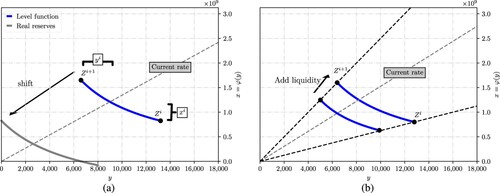
In CL pools, each tick range is a constant product pool that consists of larger reserves than the assets resting in the range because the assets resting in the tick range only need to cover marginal rate movements from its lower bound to its upper bound. The ‘virtual’ assets coordinates in a tick range $(Z^i,Z^{i+1}]$ denote the quantities of asset X and asset Y that define the constant product formula $x\times y={\kappa }^2$ in the tick range, i.e., the coordinates of the points making up the blue segment in Figure 1(a). However, the liquidity within a tick range only serves as counterparty to LT trades when the marginal rate is between the range's lower bound and its upper bound. The ‘real’ assets coordinates denote the quantities of asset X and asset Y that the LP must deposit in the tick range, i.e., the coordinates of the points making up the grey segment in Figure 1(a).

To determine the quantities $(x^i,y^i)$ that provide liquidity in the tick range $(Z^i,Z^{i+1}]$ in Figure 1(a), one shifts the level function (blue segment) from the ‘virtual’ assets coordinates to the ‘real’ assets coordinates (grey segment), where the quantity of asset Y when $Z=Z^{i+1}$ is zero, and the quantity of asset X when $Z=Z^i$ is zero. The virtual coordinates of $Z^i$ and $Z^{i+1}$ in Figure 1(a) are $({\kappa }^i\sqrt{Z^i},{\kappa }^i/\sqrt{Z^i})$ and $({\kappa }^i\sqrt{Z^{i+1}},{\kappa }^i/\sqrt{Z^{i+1}})$, respectively. Next, note that the marginal rate in the tick range $(Z^i,Z^{i+1}]$ obeys the constant product formula, and the algebraic formula to shift the level curve $x^i{y}^i=({\kappa }^i{)}^2$ is $(x^i+{\mathrm{\Delta }}^x)(y^i+{\mathrm{\Delta }}^y)=({\kappa }^i{)}^2$. Thus, the quantities provided by the LP verify the key formula $\begin{array}{r}(x^i+{\kappa }^i\sqrt{Z^i})(y^i+{\kappa }^i/\sqrt{Z^{i+1}})={\left({\kappa }^i\right)}^2,\end{array}$ which describes the behaviour of real reserves in the arc corresponding to the tick range $(Z^i,Z^{i+1}]$.

In this example, when $Z\in (Z^i,Z^{i+1}],$ the LP provides the quantities (11) $\begin{array}{r}{x}^i={\kappa }^i(Z^{1/2}-{\left(Z^i\right)}^{1/2})\text{and}{y}^i={\kappa }^i(Z^{-1/2}-{\left(Z^{i+1}\right)}^{-1/2}),\end{array}$(11) which are a function of the LP's initial wealth α, the marginal rate in the pool, and the range boundaries $Z^i$ and $Z^{i+1}$, because $\begin{array}{r}\alpha =x^i+Z{y}^i\text{and}{x}^i=y^i\frac{Z^{1/2}-{\left(Z^i\right)}^{1/2}}{Z^{-1/2}-{\left(Z^{i+1}\right)}^{-1/2}}.\end{array}$ Now, we show how to compute the depth of liquidity in a tick range provided by several LP positions. Assume a second LP provides liquidity with a different depth ${\overline{\kappa }}^i$ in the same tick range $(Z^i,Z^{i+1}]$. She deposits $({\overline{x}}^i,{\overline{y}}^i)$ so the tick range $(Z^i,Z^{i+1}]$ consists of reserves $(x^i+{\overline{x}}^i,y^i+{\overline{y}}^i)$. Use Equation (11(11) $\begin{array}{r}{x}^i={\kappa }^i(Z^{1/2}-{\left(Z^i\right)}^{1/2})\text{and}{y}^i={\kappa }^i(Z^{-1/2}-{\left(Z^{i+1}\right)}^{-1/2}),\end{array}$(11) ) to write the new depth in the tick range resulting from the two liquidity positions as $\begin{array}{r}\frac{x^i+{\overline{x}}^i}{Z^{1/2}-{\left(Z^i\right)}^{1/2}}={\kappa }^i+{\overline{\kappa }}^i.\end{array}$ Thus, one adds the depths of the individual liquidity positions in the same tick range to obtain the total depth of the liquidity in that tick range. When an LP adds liquidity in a tick range, the depth of the liquidity increases so the segment of the level function corresponding to the tick range moves up in the virtual asset coordinates; see Figure 1(b). Finally, although there is liquidity taking and liquidity provision activity in the pool, the depth of each individual position is kept constant if the LP does not deposit or withdraws assets in the range. However, liquidity provision activity may change the portion of the pool depth that the LP holds, e.g., ${\kappa }^i/({\kappa }^i+{\overline{\kappa }}^i)$ in our example; see Chapter 4 in Drissi (2023) for more details.

More generally, let Z be the rate observed in the pool, and let M be the number of LPs with liquidity resting in the pool. Denote the depth of the jth LP's liquidity $(x^{\ell ,u,j},y^{\ell ,u,j})$ posted in the range $(Z^{\ell },Z^u]$ by ${\tilde{\kappa }}^{\ell ,u,j}$. The depth ${\tilde{\kappa }}^{\ell ,u,j}$ verifies the following key formulae that define the LP provision condition in CPMs with CL: (12) $\{\begin{array}{lll}{x}^{\ell ,u,j}=0& \text{and}{y}^{\ell ,u,j}={\tilde{\kappa }}^{\ell ,u,j}({\left(Z^{\ell }\right)}^{-1/2}-{\left(Z^u\right)}^{-1/2})& \text{if}Z\le Z^{\ell },\\ x^{\ell ,u,j}={\tilde{\kappa }}^{\ell ,u,j}(Z^{1/2}-{\left(Z^{\ell }\right)}^{1/2})& \text{and}{y}^{\ell ,u,j}={\tilde{\kappa }}^{\ell ,u,j}(Z^{-1/2}-{\left(Z^u\right)}^{-1/2})& \text{if}{Z}^{\ell }<Z\le Z^u,\\ x^{\ell ,u,j}={\tilde{\kappa }}^{\ell ,u,j}({\left(Z^u\right)}^{1/2}-{\left(Z^{\ell }\right)}^{1/2})& \text{and}{y}^{\ell ,u,j}=0& \text{if}Z>Z^u.\end{array}$(12) Here, if $Z\le Z^{\ell },$ the LP provides only asset Y, i.e., $x^{\ell ,u,j}=0,$ and if $Z>Z^u,$ the LP provides only asset X, i.e., $y^{\ell ,u,j}=0$.

When an LP withdraws her liquidity, the equations in (12(12) $\{\begin{array}{lll}{x}^{\ell ,u,j}=0& \text{and}{y}^{\ell ,u,j}={\tilde{\kappa }}^{\ell ,u,j}({\left(Z^{\ell }\right)}^{-1/2}-{\left(Z^u\right)}^{-1/2})& \text{if}Z\le Z^{\ell },\\ x^{\ell ,u,j}={\tilde{\kappa }}^{\ell ,u,j}(Z^{1/2}-{\left(Z^{\ell }\right)}^{1/2})& \text{and}{y}^{\ell ,u,j}={\tilde{\kappa }}^{\ell ,u,j}(Z^{-1/2}-{\left(Z^u\right)}^{-1/2})& \text{if}{Z}^{\ell }<Z\le Z^u,\\ x^{\ell ,u,j}={\tilde{\kappa }}^{\ell ,u,j}({\left(Z^u\right)}^{1/2}-{\left(Z^{\ell }\right)}^{1/2})& \text{and}{y}^{\ell ,u,j}=0& \text{if}Z>Z^u.\end{array}$(12) ) and the prevailing exchange rate Z determine the quantities of each asset received by the LP. Here, we refer to the rate Z in the pool when the LP posts her liquidity as the position rate. In particular, the position rate is the value of the marginal rate Z used in Equation (12(12) $\{\begin{array}{lll}{x}^{\ell ,u,j}=0& \text{and}{y}^{\ell ,u,j}={\tilde{\kappa }}^{\ell ,u,j}({\left(Z^{\ell }\right)}^{-1/2}-{\left(Z^u\right)}^{-1/2})& \text{if}Z\le Z^{\ell },\\ x^{\ell ,u,j}={\tilde{\kappa }}^{\ell ,u,j}(Z^{1/2}-{\left(Z^{\ell }\right)}^{1/2})& \text{and}{y}^{\ell ,u,j}={\tilde{\kappa }}^{\ell ,u,j}(Z^{-1/2}-{\left(Z^u\right)}^{-1/2})& \text{if}{Z}^{\ell }<Z\le Z^u,\\ x^{\ell ,u,j}={\tilde{\kappa }}^{\ell ,u,j}({\left(Z^u\right)}^{1/2}-{\left(Z^{\ell }\right)}^{1/2})& \text{and}{y}^{\ell ,u,j}=0& \text{if}Z>Z^u.\end{array}$(12) ) to determine the quantities deposited by the LP in the pool.

3.1.2. LT Trading Condition

We denote the depth of the liquidity available in the pool in the range $(Z^i,Z^{i+1}]$ between two consecutive ticks by ${\kappa }^{i,i+1}$. A pool is characterized by the marginal rate Z and the distribution of the liquidity across the tick ranges, which are described by the values (13) $\begin{array}{r}{\kappa }^{i,i+1}=\sum _{j\in \{1,\dots ,M\}}\sum _{(\ell ,u)\in \{1,\dots ,N{\}}^2}{\tilde{\kappa }}^{\ell ,u,j}{\mathbb{1}}_{Z^{\ell }\le Z^i<Z^{i+1}\le Z^u},\end{array}$(13) where M is the number of liquidity providers in the pool, ${\tilde{\kappa }}_j^{\ell ,u,j}\ge 0$ is the depth of the liquidity posted by the jth LP in the range $(Z^{\ell },Z^u],$ and $\mathbb{1}$ is the indicator function. We refer to the range between two consecutive ticks that contains the rate Z as the active tick range. The value of the pool depth κ used in the LT trading condition, which defines the instantaneous and execution rates, is the depth (13(13) $\begin{array}{r}{\kappa }^{i,i+1}=\sum _{j\in \{1,\dots ,M\}}\sum _{(\ell ,u)\in \{1,\dots ,N{\}}^2}{\tilde{\kappa }}^{\ell ,u,j}{\mathbb{1}}_{Z^{\ell }\le Z^i<Z^{i+1}\le Z^u},\end{array}$(13) ) of the liquidity in the active tick range⁵.

Consequently, in CPMs with CL, one must discern between two types of depths. First, the pool depth κ which defines the LT trading condition in a specific tick range, i.e., the constant product formula (1(1) $\begin{array}{r}f(x,y)=f(x+{\mathrm{\Delta }}^x,y-{\mathrm{\Delta }}^y)={\kappa }^2.\end{array}$(1) ), the marginal rate (4(4) $\begin{array}{r}\underset{{\mathrm{\Delta }}^y\to 0}{lim}{Z}_t^{\text{bid}}\left({\mathrm{\Delta }}^y\right)=\underset{{\mathrm{\Delta }}^y\to 0}{lim}{Z}_t^{\text{ask}}\left({\mathrm{\Delta }}^y\right)=Z_t=-{\phi }^{\mathrm{\prime }}\left(y_t\right).\end{array}$(4) ), and the execution rates (3(3) $\begin{array}{r}{Z}_t^{\text{bid}}\left({\mathrm{\Delta }}^y\right)=\frac{\phi \left(y_t\right)-\phi (y_t+{\mathrm{\Delta }}^y)}{{\mathrm{\Delta }}^y}\le \frac{\phi (y_t-{\mathrm{\Delta }}^y)-\phi \left(y_t\right)}{{\mathrm{\Delta }}^y}=Z_t^{\text{ask}}\left(y\right).\end{array}$(3) ). Second, the depth ${\tilde{\kappa }}^{\ell ,u,j}$ of the individual positions held by LPs for different values of ℓ and u. In pools with CL, the depth κ is a local property, and it is a transformation of the individual depths ${\tilde{\kappa }}^{\ell ,u,j},$ see (13(13) $\begin{array}{r}{\kappa }^{i,i+1}=\sum _{j\in \{1,\dots ,M\}}\sum _{(\ell ,u)\in \{1,\dots ,N{\}}^2}{\tilde{\kappa }}^{\ell ,u,j}{\mathbb{1}}_{Z^{\ell }\le Z^i<Z^{i+1}\le Z^u},\end{array}$(13) ).

3.1.3. Fee Revenue in CPMs with CL

The transaction fees paid by LTs are distributed amongst LPs in the same proportion as their contribution to the depth in the active range. More precisely, consider an LP with liquidity resting in the range $(Z^{\ell },Z^u]$. If the active tick range is $(Z^i,Z^{i+1}]$ and $(Z^i,Z^{i+1}]\subset (Z^{\ell },Z^u]$, then for a transaction fee π paid by LTs, the jth LP, who posted depth ${\tilde{\kappa }}^{\ell ,u,j}$ in $(Z^{\ell },Z^u]$ when the pool's depth in the tick is $\kappa ={\kappa }^{i,i+1}$, receives (14) $\begin{array}{r}{\tilde{\pi }}^{\ell ,u,j}=\frac{{\tilde{\kappa }}^{\ell ,u,j}}{\kappa }\pi {\mathbb{1}}_{Z^{\ell }<Z\le Z^u}.\end{array}$(14) In CPMs without CL, this remuneration is added to the liquidity in the pool because all LPs provide liquidity in the same range $(0,+\mathrm{\infty })$ and they hold portions of the pool in the proportion of their contribution to it. However, in CPMs with CL, fee income is not automatically reinvested in the pool because LPs can provide liquidity in various ranges simultaneously, so the fees accrue in a separate account, and are paid when liquidity is withdrawn.

Similar to Section 2, we derive the continuous-time dynamics of the wealth of LPs (assuming zero fee revenue), which we study to characterize the predictable losses of LPs. In contrast to CFMs, liquidity provision in CPMs with CL is strategic. Thus, we derive the wealth dynamics for passive LPs in Subsection 3.2 and for active LPs in Subsection 3.3. Passive LPs do not change the range where they provide liquidity throughout the trading window, and active LPs continuously change the liquidity position. Finally, Subsection 3.4 uses the wealth dynamics to extend PL to CPMs with CL.

3.2. Wealth Dynamics of Passive LPs

Consider an LP with trading horizon $[0,T]$ and with initial wealth ${\alpha }_0>0$ in units of the reference asset X at the initial time t=0. The LP deposits quantities $(x_0,y_0)$ in a fixed range $(Z^{\ell },Z^u]$ that includes $Z_0$ and withdraws her liquidity at the terminal time T>0, so the initial value of her position, marked-to-market in units of X, is ${\alpha }_0=x_0+y_0{Z}_0$⁶. We (re)define the processes $(x_t{)}_{t\in [0,T]}$ and $(y_t{)}_{t\in [0,T]}$ to denote the LP's holdings in the range $(Z^{\ell },Z^u]$ of the pool, the process $({\alpha }_t{)}_{t\in [0,T]}=(x_t+y_t{Z}_t{)}_{t\in [0,T]}$ to denote the value of the LP's wealth in units of X, and $(Z_t{)}_{t\in [0,T]}$ denotes the marginal exchange rate. The depth of the LP's position is ${\tilde{\kappa }}_0$. Recall that ${\tilde{\kappa }}_0$ is constant throughout $[0,T]$ because the LP is passive; she does not withdraw or deposit additional assets and she does not change the width $Z^u-Z^{\ell }$ of her liquidity position throughout the trading window $[0,T]$.

To obtain the initial holdings of the LP in the pool when $Z_0\in (Z^{\ell },Z^u],$ one solves $\begin{array}{r}\{\begin{array}{l}{x}_0={\tilde{\kappa }}_0(Z_0^{1/2}-{\left(Z^{\ell }\right)}^{1/2}),\\ y_0={\tilde{\kappa }}_0(Z_0^{-1/2}-{\left(Z^u\right)}^{-1/2}),\\ {\alpha }_0=x_0+y_0{Z}_0,\end{array}\end{array}$ where ${\tilde{\kappa }}_0$ is the depth of the LP's liquidity in the pool, to obtain $\begin{array}{r}{x}_0={\alpha }_0{(1+\frac{Z_0^{1/2}(\left(Z^u\right){}^{1/2}-Z_0^{1/2})}{\left(Z^u\right){}^{1/2}(Z_0^{1/2}-\left(Z^{\ell }\right){}^{1/2})})}^{-1}\text{and}{y}_0=\frac{{\alpha }_0-x_0}{Z_0}.\end{array}$ At time $t\in [0,T],$ the value of the LP's holdings in units of the reference asset X is determined by the equations of the LP provision condition (15) $\begin{array}{r}\{\begin{array}{ll}{x}_t=0& \text{and}{y}_t={\tilde{\kappa }}_0({\left(Z^{\ell }\right)}^{-1/2}-{\left(Z^u\right)}^{-1/2})\text{if}{Z}_t\le Z^{\ell },\\ x_t={\tilde{\kappa }}_0(Z_t^{1/2}-{\left(Z^{\ell }\right)}^{1/2})& \text{and}{y}_t={\tilde{\kappa }}_0(Z_t^{-1/2}-{\left(Z^u\right)}^{-1/2})\text{if}{Z}^{\ell }<Z_t\le Z^u,\\ x_T={\tilde{\kappa }}_0({\left(Z^u\right)}^{1/2}-{\left(Z^{\ell }\right)}^{1/2})& \text{and}{y}_t=0\text{if}{Z}_t>Z^u,\end{array}\end{array}$(15) where $Z_t$ is the marginal rate at time t. We focus on the case where the marginal rate $Z_t$ is within the range $(Z^{\ell },Z^u]$⁷. Thus, the change in the value of the position at time $t\in [0,T]$ is (16) $\begin{array}{r}{x}_t+y_t{Z}_t-x_0-y_0{Z}_0=x_t+y_t{Z}_t-{\alpha }_0.\end{array}$(16) Equations (15(15) $\begin{array}{r}\{\begin{array}{ll}{x}_t=0& \text{and}{y}_t={\tilde{\kappa }}_0({\left(Z^{\ell }\right)}^{-1/2}-{\left(Z^u\right)}^{-1/2})\text{if}{Z}_t\le Z^{\ell },\\ x_t={\tilde{\kappa }}_0(Z_t^{1/2}-{\left(Z^{\ell }\right)}^{1/2})& \text{and}{y}_t={\tilde{\kappa }}_0(Z_t^{-1/2}-{\left(Z^u\right)}^{-1/2})\text{if}{Z}^{\ell }<Z_t\le Z^u,\\ x_T={\tilde{\kappa }}_0({\left(Z^u\right)}^{1/2}-{\left(Z^{\ell }\right)}^{1/2})& \text{and}{y}_t=0\text{if}{Z}_t>Z^u,\end{array}\end{array}$(15) ) and (16(16) $\begin{array}{r}{x}_t+y_t{Z}_t-x_0-y_0{Z}_0=x_t+y_t{Z}_t-{\alpha }_0.\end{array}$(16) ) define a payoff in units of X as a function of the marginal rate $Z_t$. Figure 2 shows the relative payoff ${\alpha }_t/{\alpha }_0$ as a function of the marginal rate for different position ranges when the position rate is $Z_0=100$. Provision of liquidity with wide spreads protects the LP from losses when $Z_t\le Z_0,$ and facilitates gains when $Z_t\ge Z_0$. Figure 2 shows that the LP's relative payoff ${\alpha }_t/{\alpha }_0$ is concave in the rate $Z_T$.

Figure 2. Payoff (15(15) $\begin{array}{r}\{\begin{array}{ll}{x}_t=0& \text{and}{y}_t={\tilde{\kappa }}_0({\left(Z^{\ell }\right)}^{-1/2}-{\left(Z^u\right)}^{-1/2})\text{if}{Z}_t\le Z^{\ell },\\ x_t={\tilde{\kappa }}_0(Z_t^{1/2}-{\left(Z^{\ell }\right)}^{1/2})& \text{and}{y}_t={\tilde{\kappa }}_0(Z_t^{-1/2}-{\left(Z^u\right)}^{-1/2})\text{if}{Z}^{\ell }<Z_t\le Z^u,\\ x_T={\tilde{\kappa }}_0({\left(Z^u\right)}^{1/2}-{\left(Z^{\ell }\right)}^{1/2})& \text{and}{y}_t=0\text{if}{Z}_t>Z^u,\end{array}\end{array}$(15) ) for an LP providing liquidity in the ranges $[95,105],[75,125]$ and $[50,150],$ around the position rate $Z_0=100$.

To obtain simple formulae for the change in the value of the LP's assets, we characterize the liquidity position of the LP with new variables $({\delta }^{\ell },{\delta }^u)$ instead of $(Z^{\ell },Z^u)$. The values of ${\delta }^{\ell }$ and ${\delta }^u$ are (percentage) shifts of $\sqrt{Z}$ and are defined with the following change of variables: (17) $\begin{array}{r}\{\begin{array}{l}{\left(Z^u\right)}^{1/2}=Z^{1/2}/(1-{\delta }^u/2),\\ {\left(Z^{\ell }\right)}^{1/2}=Z^{1/2}(1-{\delta }^{\ell }/2).\end{array}\end{array}$(17) Note that $Z^{\ell }\in [0,Z)$ so ${\delta }^{\ell }\in (0,2]$ and $Z^u\in [Z,\mathrm{\infty })$ so ${\delta }^u\in [0,2)$. Also, we require that $Z^{\ell }<Z^u$ so ${\delta }^{\ell }+{\delta }^u<{\delta }^{\ell }{\delta }^u/2$⁸. For small values of $Z^u-Z^{\ell }$ we use the approximation $\begin{array}{r}(Z^u-Z^{\ell })/Z=(1-{\delta }^u/2{)}^{-2}-{(1-{\delta }^{\ell }/2)}^2\approx {\delta }^u+{\delta }^{\ell }.\end{array}$ In the remainder of this work, we define the spread of the LP's position as ${\delta }^{\ell }+{\delta }^u=\delta$. We refer to δ as the spread because it shares similar properties to those of the spread of a market maker in LOBs. In LOBs, the spread of an LP refers to the distance between the limit orders posted on both sides of the midprice. In particular, in LOBs, market makers widen their spread when adverse selection risk increases, i.e., they post limit orders at deeper levels in the book.

We use (17(17) $\begin{array}{r}\{\begin{array}{l}{\left(Z^u\right)}^{1/2}=Z^{1/2}/(1-{\delta }^u/2),\\ {\left(Z^{\ell }\right)}^{1/2}=Z^{1/2}(1-{\delta }^{\ell }/2).\end{array}\end{array}$(17) ) to write the change in the value of the assets as a function of the spread of the position and as a function of changes in the value of Z and of $\sqrt{Z}$. First, use the second equation in (12(12) $\{\begin{array}{lll}{x}^{\ell ,u,j}=0& \text{and}{y}^{\ell ,u,j}={\tilde{\kappa }}^{\ell ,u,j}({\left(Z^{\ell }\right)}^{-1/2}-{\left(Z^u\right)}^{-1/2})& \text{if}Z\le Z^{\ell },\\ x^{\ell ,u,j}={\tilde{\kappa }}^{\ell ,u,j}(Z^{1/2}-{\left(Z^{\ell }\right)}^{1/2})& \text{and}{y}^{\ell ,u,j}={\tilde{\kappa }}^{\ell ,u,j}(Z^{-1/2}-{\left(Z^u\right)}^{-1/2})& \text{if}{Z}^{\ell }<Z\le Z^u,\\ x^{\ell ,u,j}={\tilde{\kappa }}^{\ell ,u,j}({\left(Z^u\right)}^{1/2}-{\left(Z^{\ell }\right)}^{1/2})& \text{and}{y}^{\ell ,u,j}=0& \text{if}Z>Z^u.\end{array}$(12) ) and in (17(17) $\begin{array}{r}\{\begin{array}{l}{\left(Z^u\right)}^{1/2}=Z^{1/2}/(1-{\delta }^u/2),\\ {\left(Z^{\ell }\right)}^{1/2}=Z^{1/2}(1-{\delta }^{\ell }/2).\end{array}\end{array}$(17) ) to write the depth ${\tilde{\kappa }}_0$ of the LP's liquidity as (18) $\begin{array}{r}{\tilde{\kappa }}_0=2{\alpha }_0\left(\frac{1}{{\delta }_0^{\ell }+{\delta }_0^u}\right)Z_0^{-1/2}.\end{array}$(18) Second, use the definition (17(17) $\begin{array}{r}\{\begin{array}{l}{\left(Z^u\right)}^{1/2}=Z^{1/2}/(1-{\delta }^u/2),\\ {\left(Z^{\ell }\right)}^{1/2}=Z^{1/2}(1-{\delta }^{\ell }/2).\end{array}\end{array}$(17) ) to write the initial quantities $(x_0,y_0)$ that the LP deposits in the pool in the simpler form (19) $\begin{array}{r}{x}_0=\frac{{\delta }_0^{\ell }}{{\delta }_0^{\ell }+{\delta }_0^u}{\alpha }_0\text{and}{y}_0{Z}_0=\frac{{\delta }_0^u}{{\delta }_0^{\ell }+{\delta }_0^u}{\alpha }_0.\end{array}$(19) Finally, use (15(15) $\begin{array}{r}\{\begin{array}{ll}{x}_t=0& \text{and}{y}_t={\tilde{\kappa }}_0({\left(Z^{\ell }\right)}^{-1/2}-{\left(Z^u\right)}^{-1/2})\text{if}{Z}_t\le Z^{\ell },\\ x_t={\tilde{\kappa }}_0(Z_t^{1/2}-{\left(Z^{\ell }\right)}^{1/2})& \text{and}{y}_t={\tilde{\kappa }}_0(Z_t^{-1/2}-{\left(Z^u\right)}^{-1/2})\text{if}{Z}^{\ell }<Z_t\le Z^u,\\ x_T={\tilde{\kappa }}_0({\left(Z^u\right)}^{1/2}-{\left(Z^{\ell }\right)}^{1/2})& \text{and}{y}_t=0\text{if}{Z}_t>Z^u,\end{array}\end{array}$(15) ) and (18(18) $\begin{array}{r}{\tilde{\kappa }}_0=2{\alpha }_0\left(\frac{1}{{\delta }_0^{\ell }+{\delta }_0^u}\right)Z_0^{-1/2}.\end{array}$(18) ) to write the quantities $(x_t,y_t)$ that the LP holds in the pool as $\begin{array}{rl}& \{\begin{array}{l}{x}_t={\tilde{\kappa }}_0(Z_t^{1/2}-{\left(Z^{\ell }\right)}^{1/2}),\\ y_t{Z}_t={\tilde{\kappa }}_0(Z_t^{1/2}-Z_t{\left(Z^u\right)}^{-1/2}),\end{array}\\ & ⟹\{\begin{array}{l}{\displaystyle x_t=\frac{2{\alpha }_0}{{\delta }_0^{\ell }+{\delta }_0^u}(\frac{Z_t^{1/2}}{Z_0^{1/2}}-(1-\frac{{\delta }_0^{\ell }}{2})),}\\ {\displaystyle y_t{Z}_t=\frac{2{\alpha }_0}{{\delta }_0^{\ell }+{\delta }_0^u}(\frac{Z_t^{1/2}}{Z_0^{1/2}}-\frac{Z_t}{Z_0}(1-\frac{{\delta }_0^u}{2})).}\end{array}\end{array}$ The change in the value of the LP's position between times 0 and t is (20) $\begin{array}{r}{\alpha }_t-{\alpha }_0=x_t+y_t{Z}_t-{\alpha }_0=2{\alpha }_0\left(\frac{1}{{\delta }_0^{\ell }+{\delta }_0^u}\right)(2\frac{Z_t^{1/2}-Z_0^{1/2}}{Z_0^{1/2}}-\frac{Z_t-Z_0}{Z_0}(1-\frac{{\delta }_0^u}{2})),\end{array}$(20) which shows that the change in the value of the LP's holdings in the CL pool depends on the change in Z and $\sqrt{Z}$, and it is inversely proportional to the spread δ of the position; large values of the spread reduce the risk of the LP's position. Below, we show that the changes in $\sqrt{Z}$ in (20(20) $\begin{array}{r}{\alpha }_t-{\alpha }_0=x_t+y_t{Z}_t-{\alpha }_0=2{\alpha }_0\left(\frac{1}{{\delta }_0^{\ell }+{\delta }_0^u}\right)(2\frac{Z_t^{1/2}-Z_0^{1/2}}{Z_0^{1/2}}-\frac{Z_t-Z_0}{Z_0}(1-\frac{{\delta }_0^u}{2})),\end{array}$(20) ) are the source of PL, which is the PL component in the wealth of LPs. The dependence of the wealth of LPs on the changes in $\sqrt{Z}$ is a direct consequence of the constant product formula and PL is a consequence of the convexity of the corresponding level function.

3.3. Wealth Dynamics of Active LPs

Here, we generalize the analysis of Section 3.2 to any dynamic or passive liquidity provision strategy. More precisely, we define the shift processes $({\delta }_t^{\ell }{)}_{t\in [0,T]}$ and $({\delta }_t^u{)}_{t\in [0,T]}$ that determine the dynamic spread of the strategy that the LP implements, i.e., $\begin{array}{r}\{\begin{array}{l}{\left(Z_t^u\right)}^{1/2}=Z_t^{1/2}/(1-{\delta }_t^u/2),\\ {\left(Z_t^{\ell }\right)}^{1/2}=Z_t^{1/2}(1-{\delta }_t^{\ell }/2),\end{array}\end{array}$ where $(Z_t^{\ell }{)}_{t\in [0,T]}$ and $(Z_t^u{)}_{t\in [0,T]}$ are the processes that describe the active strategy of the LP throughout the trading window $[0,T]$. The set of admissible liquidity provision strategies is $\begin{array}{rl}\mathcal{A}& =\left\{{({\delta }_t^{\ell },{\delta }_t^u)}_{t\in [0,T]}\right|(0,2]\text{-valued},\mathbb{F}\text{-adapted},\\ & \text{and}{\int }_0^T(|{\delta }_t^{\ell }{|}^{\pm 2}+|{\delta }_t^u{|}^{\pm 2})\mathrm{d}t<+\mathrm{\infty }\mathbb{P}\text{--a.s.}\}.\end{array}$ Recall that we do not yet assume dynamics for the marginal rate. Let $({\kappa }_t{)}_{t\in [0,T]}$ be the depth process of the LP's dynamic position in the pool with initial value ${\kappa }_0$ in (18(18) $\begin{array}{r}{\tilde{\kappa }}_0=2{\alpha }_0\left(\frac{1}{{\delta }_0^{\ell }+{\delta }_0^u}\right)Z_0^{-1/2}.\end{array}$(18) ).

We assume that the LP continuously tracks the rate Z so for all $t\in [0,T]$ and that the marginal rate is within the LP's range, i.e., $Z_t\in (Z_t^{\ell },Z_t^u]$. Let $(x_t^{\ell ,u}{)}_{t\in [0,T]}$ and $(y_t^{\ell ,u}{)}_{t\in [0,T]}$ be the holdings of the LP in the pool corresponding to the active strategy $({\delta }_t^{\ell },{\delta }_t^u{)}_{t\in [0,T]}$, where the initial values $x_0$ and $y_0$ are in (19(19) $\begin{array}{r}{x}_0=\frac{{\delta }_0^{\ell }}{{\delta }_0^{\ell }+{\delta }_0^u}{\alpha }_0\text{and}{y}_0{Z}_0=\frac{{\delta }_0^u}{{\delta }_0^{\ell }+{\delta }_0^u}{\alpha }_0.\end{array}$(19) ). Finally, let $({\alpha }_t^{\ell ,u}{)}_{t\in [0,T]}$ be the cash process of the LP with initial value ${\alpha }_0=x_0+y_0{Z}_0$.

The dynamic strategy $({\delta }_t^{\ell },{\delta }_t^u{)}_{t\in [0,T]}$ of the LP consists in holding $x_t^{\ell ,u}$ units of the reference asset X, and $y_t^{\ell ,u}$ units of the asset Y at each time t in the (dynamic) range $(Z_t^{\ell },Z_t^u],$ where (21) $\begin{array}{r}{x}_t^{\ell ,u}=\frac{{\delta }_t^{\ell }}{{\delta }_t^{\ell }+{\delta }_t^u}{\alpha }_t^{\ell ,u}\text{and}{y}_t^{\ell ,u}=\frac{{\delta }_t^u}{Z_t({\delta }_t^{\ell }+{\delta }_t^u)}{\alpha }_t^{\ell ,u}.\end{array}$(21) These holdings correspond to a liquidity position with depth $\begin{array}{r}{\tilde{\kappa }}_t=2{\alpha }_t^{\ell ,u}\left(\frac{1}{{\delta }_t^{\ell }+{\delta }_t^u}\right)Z_t^{-1/2}.\end{array}$ Now, to obtain the infinitesimal change in the value of the LP's position, recall that Z is an Itô process and use Itô's lemma to write $\begin{array}{r}\mathrm{d}{Z}_t^{1/2}=\frac{1}{2}{Z}_t^{-1/2}\mathrm{d}{Z}_t-\frac{1}{8}{Z}_t^{-3/2}\mathrm{d}{〈Z,Z〉}_t,\end{array}$ and write the infinitesimal increments of ${\alpha }^{\ell ,u}$ as the continuous-time version of Equation (20(20) $\begin{array}{r}{\alpha }_t-{\alpha }_0=x_t+y_t{Z}_t-{\alpha }_0=2{\alpha }_0\left(\frac{1}{{\delta }_0^{\ell }+{\delta }_0^u}\right)(2\frac{Z_t^{1/2}-Z_0^{1/2}}{Z_0^{1/2}}-\frac{Z_t-Z_0}{Z_0}(1-\frac{{\delta }_0^u}{2})),\end{array}$(20) ): (22) $\begin{array}{rl}\mathrm{d}{\alpha }_t^{\ell ,u}& =2{\alpha }_t^{\ell ,u}\left(\frac{1}{{\delta }_t^{\ell }+{\delta }_t^u}\right)(2\frac{\mathrm{d}{Z}_t^{1/2}}{Z_t^{1/2}}-\frac{\mathrm{d}{Z}_t}{Z_t}(1-\frac{{\delta }_t^u}{2}))\\ & =2{\alpha }_t^{\ell ,u}\left(\frac{1}{{\delta }_t^{\ell }+{\delta }_t^u}\right)(-\frac{1}{4Z_t^2}\mathrm{d}{〈Z,Z〉}_t+\frac{{\delta }_t^u}{2}\frac{\mathrm{d}{Z}_t}{Z_t}).\end{array}$(22) Thus, for any liquidity provision strategy characterized by the shifts $({\delta }_t^{\ell }{)}_{t\in [0,T]}$ and $({\delta }_t^u{)}_{t\in [0,T]}$, the dynamics in (22(22) $\begin{array}{rl}\mathrm{d}{\alpha }_t^{\ell ,u}& =2{\alpha }_t^{\ell ,u}\left(\frac{1}{{\delta }_t^{\ell }+{\delta }_t^u}\right)(2\frac{\mathrm{d}{Z}_t^{1/2}}{Z_t^{1/2}}-\frac{\mathrm{d}{Z}_t}{Z_t}(1-\frac{{\delta }_t^u}{2}))\\ & =2{\alpha }_t^{\ell ,u}\left(\frac{1}{{\delta }_t^{\ell }+{\delta }_t^u}\right)(-\frac{1}{4Z_t^2}\mathrm{d}{〈Z,Z〉}_t+\frac{{\delta }_t^u}{2}\frac{\mathrm{d}{Z}_t}{Z_t}).\end{array}$(22) ) describe the dynamics of the value of the LP's holdings in the pool.

3.4. Predictable Loss in CPMs with CL

Here, we extend PL to the specific case of CPMs with CL, which requires to account for the spread of the LP's position. For simplicity, asset X is the numeraire and the LP values her wealth in terms of X, so only asset Y drives uncertainty in the LP's wealth. Similar to PL for CFMs, we consider a self-financed portfolio $({\alpha }_t^{\text{D}}{)}_{t\in [0,T]}$ that is continuously rebalanced to mimic the LP's holdings in (21(21) $\begin{array}{r}{x}_t^{\ell ,u}=\frac{{\delta }_t^{\ell }}{{\delta }_t^{\ell }+{\delta }_t^u}{\alpha }_t^{\ell ,u}\text{and}{y}_t^{\ell ,u}=\frac{{\delta }_t^u}{Z_t({\delta }_t^{\ell }+{\delta }_t^u)}{\alpha }_t^{\ell ,u}.\end{array}$(21) ) and invests any additional cash in a risk-free account with $r\ge 0$, and we write (23) $\begin{array}{r}\mathrm{d}{\alpha }_t^{\text{D}}=y_t^{\ell ,u}\mathrm{d}{Z}_t=\frac{{\delta }_t^u}{Z_t({\delta }_t^{\ell }+{\delta }_t^u)}{\alpha }_t^{\ell ,u}\mathrm{d}{Z}_t+({\alpha }_t^{\text{D}}-{\alpha }_t)r\mathrm{d}t.\end{array}$(23) After similar steps to those above, one shows that the process $({\alpha }_t^{\text{D}}-{\alpha }_t{)}_{t\in [0,T]}$ is increasing with initial value ${\alpha }_0^{\text{D}}-{\alpha }_0=0$. Next, define the PL process $({\mathrm{P}\mathrm{L}}_t^{\ell ,u}{)}_{t\in [0,T]}$ and write (24) $\begin{array}{r}{\mathrm{P}\mathrm{L}}_t^{\ell ,u}={\alpha }_t^{\ell ,u}-{\alpha }_t^{\text{D}}=-\underset{\text{Convexity cost}\ge 0}{\underbrace{{\int }_0^t\frac{{\alpha }_s^{\ell ,u}}{2({\delta }_s^{\ell }+{\delta }_s^u)Z_s^2}\mathrm{d}{〈Z,Z〉}_s}}-\underset{\text{Opportunity cost}\ge 0}{\underbrace{{\int }_0^t({\alpha }_t^{\text{D}}-{\alpha }_t)r\mathrm{d}s}}\le 0.\end{array}$(24) In contrast to IL, which has been derived for CPMs with CL by Heimbach, Schertenleib, and Wattenhofer (2022) and Loesch et al. (2021) and which shares similar properties to those of IL in CFMs, PL is a predictable and unhedgeable loss component which is key to measuring the profitability of liquidity provision in liquidity pooling protocols with CL. Below, we study the properties of PL when the marginal rate follows geometric Brownian dynamics with drift.

3.4.1. PL and Volatility

Assume that the rate process $(Z_t{)}_{t\in [0,T]}$ follows the geometric Brownian dynamics $\begin{array}{r}\mathrm{d}{Z}_t=\mu Z_t\mathrm{d}t+\sigma Z_t\mathrm{d}{W}_t,\end{array}$ where the volatility parameter σ is a nonnegative constant, the trend parameter μ is a constant, and $(W_t{)}_{t\in [0,T]}$ is a standard Brownian motion.

For simplicity, consider that the risk-free rate r is zero so the opportunity cost component of PL is zero. Thus, the dynamics of the value of the LP's position is (25) $\begin{array}{r}\mathrm{d}{\alpha }_t^{\ell ,u}=\frac{{\alpha }_t^{\ell ,u}}{{\delta }_t}(-\frac{{\sigma }^2}{2}\mathrm{d}t+\mu {\delta }_t^u\mathrm{d}t+\sigma {\delta }_t^u\mathrm{d}{W}_t),\end{array}$(25) where PL in (24(24) $\begin{array}{r}{\mathrm{P}\mathrm{L}}_t^{\ell ,u}={\alpha }_t^{\ell ,u}-{\alpha }_t^{\text{D}}=-\underset{\text{Convexity cost}\ge 0}{\underbrace{{\int }_0^t\frac{{\alpha }_s^{\ell ,u}}{2({\delta }_s^{\ell }+{\delta }_s^u)Z_s^2}\mathrm{d}{〈Z,Z〉}_s}}-\underset{\text{Opportunity cost}\ge 0}{\underbrace{{\int }_0^t({\alpha }_t^{\text{D}}-{\alpha }_t)r\mathrm{d}s}}\le 0.\end{array}$(24) ) is (26) $\begin{array}{r}{\mathrm{P}\mathrm{L}}_t^{\ell ,u}=-\frac{{\sigma }^2}{2}{\int }_0^t\frac{{\alpha }_s^{\ell ,u}}{{\delta }_s}\mathrm{d}s\le 0.\end{array}$(26) Clearly, the magnitude of PL incurred by the LP's position increases with the volatility of the rate Z. Thus, one expects an optimal liquidity provision model to adjust the spread of the position as a function of volatility. Moreover, the dynamics in (25(25) $\begin{array}{r}\mathrm{d}{\alpha }_t^{\ell ,u}=\frac{{\alpha }_t^{\ell ,u}}{{\delta }_t}(-\frac{{\sigma }^2}{2}\mathrm{d}t+\mu {\delta }_t^u\mathrm{d}t+\sigma {\delta }_t^u\mathrm{d}{W}_t),\end{array}$(25) ) and (26(26) $\begin{array}{r}{\mathrm{P}\mathrm{L}}_t^{\ell ,u}=-\frac{{\sigma }^2}{2}{\int }_0^t\frac{{\alpha }_s^{\ell ,u}}{{\delta }_s}\mathrm{d}s\le 0.\end{array}$(26) ) show how the LP can reduce PL by increasing the spread of the position in the pool. The spread $\delta ={\delta }^{\ell }+{\delta }^u$ is maximal (and equal to 4) when ${\delta }^{\ell }=2$ and ${\delta }^u=2,$ because it corresponds to the position $(Z^{\ell },Z^u]=(0,\mathrm{\infty }]$ with the largest spread. If the spread δ is maximal and the risk-free rate is zero, then PL is minimal (but not zero) and we denote it by ${\mathrm{P}\mathrm{L}}_t^{\text{min}}$. Recall that PL is given by ${\mathrm{P}\mathrm{L}}_t^{\ell ,u}={\alpha }_t^{\ell ,u}-{\alpha }_t^{\text{D}}$, so when ${\delta }^{\ell }={\delta }^u=2$ and r=0 we have that $\mathbb{E}\left[{\mathrm{P}\mathrm{L}}_T^{\ell ,u}\right]\le \mathbb{E}\left[{\mathrm{P}\mathrm{L}}_T^{\text{min}}\right]$, where $\begin{array}{r}\mathbb{E}\left[{\mathrm{P}\mathrm{L}}_T^{\text{min}}\right]=-\frac{{\sigma }^2}{8\hat{\mu }}{\alpha }_0(\exp \left(\hat{\mu }T\right)-1)\le 0,\text{if}\hat{\mu }=\frac{\mu }{2}-\frac{{\sigma }^2}{4}\ne 0,\end{array}$ and $\begin{array}{r}\mathbb{E}\left[{\mathrm{P}\mathrm{L}}_T^{\text{min}}\right]=-{\sigma }^2{\alpha }_{0}T/8,\text{if}\hat{\mu }=0.\end{array}$ In contrast to the alternative portfolio ${\alpha }^{\text{D}}$, the negative component in the trend of the LP's holdings ${\alpha }^{\ell ,u}$ scales with the volatility σ; see (25(25) $\begin{array}{r}\mathrm{d}{\alpha }_t^{\ell ,u}=\frac{{\alpha }_t^{\ell ,u}}{{\delta }_t}(-\frac{{\sigma }^2}{2}\mathrm{d}t+\mu {\delta }_t^u\mathrm{d}t+\sigma {\delta }_t^u\mathrm{d}{W}_t),\end{array}$(25) ). When volatility becomes arbitrarily high, the LP expects to lose at least her initial wealth because $\begin{array}{r}\underset{\sigma \to +\mathrm{\infty }}{lim}\mathbb{E}\left[{\mathrm{P}\mathrm{L}}_T^{\ell ,u}\right]\le \underset{\sigma \to +\mathrm{\infty }}{lim}\mathbb{E}\left[{\mathrm{P}\mathrm{L}}_T^{\text{min}}\right]=-{\alpha }_0.\end{array}$

3.4.2. PL, Drift, and Trading Horizon

Next, we discuss further the PL incurred by the LP for various ranges of the drift of the rate and for long trading horizons and with ${\delta }^{\ell }={\delta }^u=2$ and r=0. When the trend in the rate Z is $\mu \ge {\sigma }^2/2,$ the value of the holdings ${\alpha }^{\ell ,u}$ in the pool and the value of the alternative portfolio ${\alpha }^{\text{D}}$ increase because of the positive trend in their dynamics. However, the value of the alternative portfolio ${\alpha }^{\text{D}}$ increases faster than that of ${\alpha }^{\ell ,u}$, hence, as the LP's trading horizon becomes arbitrarily large, we have that $\begin{array}{r}\underset{T\to +\mathrm{\infty }}{lim}\mathbb{E}\left[{\mathrm{P}\mathrm{L}}_T^{\ell ,u}\right]=-\mathrm{\infty },\end{array}$ that is, the difference between the value of the alternative portfolio and that of the holdings in the pool is infinite; see first panel in Figure 3.

Figure 3. Simulated paths for the position value ${\alpha }_t^{\text{min}}$ and the alternative portfolio ${\overline{\alpha }}_t^{\text{min}}$. The position value ${\alpha }_t^{\text{min}}$ follows the dynamics in (25(25) $\begin{array}{r}\mathrm{d}{\alpha }_t^{\ell ,u}=\frac{{\alpha }_t^{\ell ,u}}{{\delta }_t}(-\frac{{\sigma }^2}{2}\mathrm{d}t+\mu {\delta }_t^u\mathrm{d}t+\sigma {\delta }_t^u\mathrm{d}{W}_t),\end{array}$(25) ) and ${\overline{\alpha }}_t^{\text{min}}$ follows the dynamics in (23(23) $\begin{array}{r}\mathrm{d}{\alpha }_t^{\text{D}}=y_t^{\ell ,u}\mathrm{d}{Z}_t=\frac{{\delta }_t^u}{Z_t({\delta }_t^{\ell }+{\delta }_t^u)}{\alpha }_t^{\ell ,u}\mathrm{d}{Z}_t+({\alpha }_t^{\text{D}}-{\alpha }_t)r\mathrm{d}t.\end{array}$(23) ) when ${\delta }^{\ell }={\delta }^u=2$ and r=0. Left panel: $\mu =0.02\mathrm{\%}$ and $\sigma =2\mathrm{\%}$. Right panel: $\mu =-0.02\mathrm{\%}$ and $\sigma =3\mathrm{\%}$.

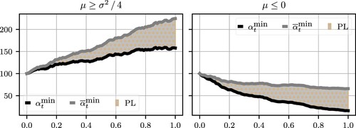
On the other hand, if $\mu <{\sigma }^2/2$, we have that $\begin{array}{r}\underset{T\to +\mathrm{\infty }}{lim}\mathbb{E}\left[{\mathrm{P}\mathrm{L}}_T^{\ell ,u}\right]\le \underset{T\to +\mathrm{\infty }}{lim}\mathbb{E}\left[{\mathrm{P}\mathrm{L}}_T^{\text{min}}\right]=\frac{{\alpha }_0{\sigma }^2}{4\mu -2{\sigma }^2}<0.\end{array}$ In particular, the expected minimum PL decreases when the trend is large and negative as both portfolios ${\alpha }^{\ell ,u}$ and ${\alpha }^{\text{D}}$ incur large losses; see second panel in Figure 3.

Finally, when $\mu =0,$ the expected minimum PL is $\begin{array}{r}\mathbb{E}\left[{\mathrm{P}\mathrm{L}}_T^{\text{min}}\right]={\alpha }_0(\exp (-\frac{1}{4}{\sigma }^{2}T)-1),\end{array}$ in which case the LP expects to lose her initial wealth when volatility or the time horizon becomes arbitrarily high.

4. Empirical Analysis of PL in Uniswap V3

This section studies PL in the pool ETH/USDC $0.3\mathrm{\%}$ of the CPM Uniswap v3 which implements CL. Uniswap v3 pools can be created with different values of the LT trading fee, e.g., $0.01\mathrm{\%},$ $0.05\mathrm{\%},$ $0.30\mathrm{\%},$ or $1\mathrm{\%},$ called fee tiers. Additionally, different pools with the same asset pair can coexist if they have different fee tiers. Once a pool is created, its fee tier does not change. ETH represents Ether, the Ethereum blockchain native currency, and USDC represents USD coin, a currency fully backed by U.S. Dollars (USD). The fee paid by LTs in the pool we consider is $0.3\mathrm{\%}$ of the trade size; the fee is deducted from the quantity paid into the pool by the LT and distributed among LPs; see Equation (14(14) $\begin{array}{r}{\tilde{\pi }}^{\ell ,u,j}=\frac{{\tilde{\kappa }}^{\ell ,u,j}}{\kappa }\pi {\mathbb{1}}_{Z^{\ell }<Z\le Z^u}.\end{array}$(14) ). Table 1 provides descriptive statistics of the transaction data (liquidity taking trades and liquidity provision operations) we use.

Table 1. LT and liquidity provision activity in the ETH/USDC pool between 5 May 2021 and 10 January 2023: count of LT transactions and LP operations in the pool, size of LT transactions and LP operations in the pool in USD, and average liquidity taking and provision frequency.

	LT	LP
Number of instructions	390,378	158,459
Total USD volume	≈$ 67.18 $\times {10}^9$	≈$ 142.62 $\times {10}^9$
Average trading frequency	136 seconds	337 seconds

To study the profitability of liquidity provision in the pool that we consider, we select operation pairs that consist of first providing and then withdrawing the same depth of liquidity $\tilde{\kappa }$ by the same LP at two different points in time⁹. The operations that we select represent approximately $66\mathrm{\%}$ of all LP operations. Next, for every LP position in the set that we consider, we compute the expected PL as a percentage of the LP's initial wealth, i.e., we compute $\begin{array}{r}\mathbb{E}\left[{\mathrm{P}\mathrm{L}}_T^{\ell ,u}\right]/{\alpha }_0=\frac{1}{\delta }(\exp (-\frac{{\sigma }^2}{8}T)-1),\end{array}$ where ${\alpha }_0$ is the LP's initial wealth, T is her trading horizon, δ is the (fixed) spread, and σ is the daily standard deviation based on one month of returns prior to the start date of the LP's position¹⁰. Table 2 shows the average PL and the realized fee revenue of LPs, and Figure 4 shows the distribution of both metrics. Clearly, the fee revenue in the pool that we consider does not cover PL.

Figure 4. Distribution of PL and fee revenue for the historical LP transactions in the ETH/USDC pool.

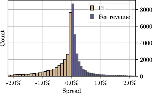
Table 2. LP operations statistics in the ETH/USDC pool with transaction data of 5,156 different LPs between 5 May 2021 and 10 January 2023. Performance includes transaction fees and excludes gas fees. PL and fee revenue are normalized to denote daily performance.

	Average	Standard deviation
Number of transactions per LP	2.61	14.26
PL	$-0.70\mathrm{\%}$	$1.01\mathrm{\%}$
Fee revenue	$0.27\mathrm{\%}$	$0.38\mathrm{\%}$
Hold time	9.70 days	16.71 days
Spread	$38.21\mathrm{\%}$	$39.77\mathrm{\%}$

In an efficient market, one would expect LPs to be driven out of the market unless, everything else being equal, the fees paid by LTs increase (and gas fees decrease). With the current fee structure and fee levels, LPs are overexposed to PL during periods of heightened volatility of the rate of the pool. Currently, the fee structure in CFMs cannot lead to efficient and resilient markets because liquidity will be scarce during times of high volatility and, in the long term, LPs will withdraw from the market.

A potential solution is one or a combination of the following two proposals. First, increase the level of fixed fees paid by LTs in CFMs or implement a dynamic structure where fees are an increasing function of the PL; the PL function depends on the volatility of the rate, convexity of the pool's trading function, and opportunity cost of the LP's wealth¹¹. Second, propose efficient AMM designs beyond CFMs where LPs express their views on the liquidity taking flow in the price of liquidity, so the resulting trading function accommodates both LPs and LTs; see Cartea et al. (2023) for research in this direction. Clearly, a change in fee level and fee structure will affect trading activity in CFMs. In particular, an increase in fees will impact the demand for liquidity because it will be more expensive for LTs to trade, while, on the other hand, it will incentivise liquidity provision because compensation will increase, on average – it is a challenging problem to find a fee structure that provides an equilibrium where activity is not hindered, the market is resilient, and the rates of the pool are efficient.

5. Conclusions

This paper discussed the microstructural properties for liquidity takers and providers in CFMs. We introduced predictable loss (PL) as a new measure of loss in liquidity provision activity in CFMs and in CPMs with CL. Our analysis of Uniswap v3 data showed that LPs trade at a loss in the pool we consider, and that our strategy significantly improves performance.

Acknowledgements

We are grateful to Tarek Abou Zeid, Álvaro Arroyo, Sam Cohen, Patrick Chang, Mihai Cucuringu, Olivier Guéant, Anthony Ledford, Andre Rzym, and Leandro Sánchez-Betancourt, for insightful comments.

Disclosure statement

No potential conflict of interest was reported by the author(s).

Additional information

Funding

The authors thank the Fintech Dauphine Chair, in partnership with Mazars and Crédit Agricole CIB, for their financial support. We are also grateful to seminar participants at Oxford, the OMI, the Oxford Victoria Seminar, and the DeFi Research Group. FD is grateful to the Oxford-Man Institute's generosity and hospitality. MM acknowledges financial support from the EPSRC Centre for Doctoral Training in Mathematics of Random Systems: Analysis, Modelling and Simulation (EP/S023925/1).

Notes

1 The level function is akin to the forward exchange function in Angeris et al. (2022).

2 These assumptions simplify the equations for IL and PL in CFMs because liquidity provision activity changes κ which changes the level function ${\phi }_{\kappa }$. We expect the results that we state below to hold when there is liquidity provision activity; for instance, it is straightforward to generalize the results for IL and PL when κ is a counting process that models arrivals of deposits and withdrawals; see Appendix.

3 PL is inevitable while the LP's holdings are in the pool.

4 In LOBs, a tick is the smallest price increment.

5 When the rate Z crosses a tick as a result of an LT transaction, the order is executed as two separate transactions; if it crosses multiple ticks, the order is executed as multiple transactions. In particular, each transaction will use the depth κ of each tick range.

6 In the two cases where liquidity is provided in a range that does not include the rate $Z_0$, the initial holdings are $\{\begin{array}{lll}{x}_0=0& \text{and}{y}_0={\alpha }_0/Z_0& \text{if}{Z}_0\le Z^{\ell },\\ x_0={\alpha }_0& \text{and}{y}_0=0& \text{if}{Z}_0>Z^u.\end{array}$

7 Later, we mainly focus on dynamic strategies where the LP targets the rate $Z_t$.

8 In the general case where one does not require $Z\in (Z^{\ell },Z^u]$, the conditions are ${\delta }^{\ell }\in (-\mathrm{\infty },2]$, ${\delta }^u\in [-\mathrm{\infty },2)$, and ${\delta }^{\ell }+{\delta }^u<{\delta }^{\ell }{\delta }^u/2$.

9 In blockchain data, every transaction is associated to a unique wallet address.

10 We assume $\mu =0$ in (25(25) $\begin{array}{r}\mathrm{d}{\alpha }_t^{\ell ,u}=\frac{{\alpha }_t^{\ell ,u}}{{\delta }_t}(-\frac{{\sigma }^2}{2}\mathrm{d}t+\mu {\delta }_t^u\mathrm{d}t+\sigma {\delta }_t^u\mathrm{d}{W}_t),\end{array}$(25) ).

11 In LOBs, this dynamic adjustment of the fee is endogenous because liquidity providers increase the spread between the best bid and best ask when volatility of the midprice increases.

Appendix. Impermanent loss with stochastic liquidity provision activity

Here, we generalize IL to the case when liquidity provision activity is stochastic. Consider an LP who deposits quantities $(x_0,y_0)$ in a CFM pool for the pair of assets X and Y . Similar to Section 2.3, the LP's position is self-financed, so she does not deposit or withdraw additional assets throughout a trading horizon $[0,T]$. In contrast to Section 2.3, we model liquidity provision activity as the sum of two Poisson processes that count liquidity provision and liquidity withdrawal operations in the CFM pool. Let $(N_t^{\text{deposit}}{)}_{t\in [0,T]}$ be a Poisson process that models the arrival of LP operations that deposit liquidity, and $(N_t^{\text{withdraw}}{)}_{t\in [0,T]}$ be a Poisson process that models the arrival of LP operations that withdraw liquidity. Both processes have some (possibly stochastic) intensity.

We assume that the liquidity provision operations are for a fixed liquidity depth $\xi >0$ and we assume that $(\kappa {)}_{t\in [0,T]}$ has the dynamics $\begin{array}{r}\mathrm{d}{\kappa }_s=\xi \mathrm{d}{N}_t^{\text{deposit}}-\xi \mathrm{d}{N}_t^{\text{withdraw}},\end{array}$ and write IL in (10(10) $\begin{array}{r}{\mathrm{I}\mathrm{L}}_t={\alpha }_t-{\alpha }_t^{\text{P}}=-(\phi \left(y_0\right)-\phi \left(y_t\right)-{\phi }^{\mathrm{\prime }}(y_t\left)(y_0-y_t)\right).\end{array}$(10) ) as $\begin{array}{rl}{\mathrm{I}\mathrm{L}}_t& ={\alpha }_t-{\alpha }_t^{\text{P}}\\ & =-{\int }_0^t({\phi }_{{\kappa }_s-\xi }\left(y_{s-}\right)-{\phi }_{{\kappa }_s-\xi }\left(y_s\right)-{\phi }_{{\kappa }_s-\xi }^{\mathrm{\prime }}(y_s\left)(y_{s-}-y_s)\right)\mathrm{d}{N}_s^{\text{withdraw}}\\ & -{\int }_0^t({\phi }_{{\kappa }_s+\xi }\left(y_{s-}\right)-{\phi }_{{\kappa }_s+\xi }\left(y_s\right)-{\phi }_{{\kappa }_s+\xi }^{\mathrm{\prime }}(y_s\left)(y_{s-}-y_s)\right)\mathrm{d}{N}_s^{\text{deposit}}\\ & -{\int }_0^t({\phi }_{{\kappa }_s}\left(y_{s-}\right)-{\phi }_{{\kappa }_s}\left(y_s\right)-{\phi }_{{\kappa }_s}^{\mathrm{\prime }}(y_s\left)(y_{s-}-y_s)\right)(1-\mathrm{d}{N}_s^{\text{withdraw}})\\ & -{\int }_0^t({\phi }_{{\kappa }_s}\left(y_{s-}\right)-{\phi }_{{\kappa }_s}\left(y_s\right)-{\phi }_{{\kappa }_s}^{\mathrm{\prime }}(y_s\left)(y_{s-}-y_s)\right)(1-\mathrm{d}{N}_s^{\text{deposit}}),\end{array}$ which is always non-positive because ${\phi }_{\kappa }$ is convex for any value of the depth κ.

References

- Adams, H., N. Zinsmeister, M. Salem, R. Keefer, and D. Robinson. 2021. “Uniswap v3 core.” Technical Report.
- Angeris, G., A. Agrawal, A. Evans, T. Chitra, and S. Boyd. 2022. “Constant Function Market Makers: Multi-Asset Trades Via Convex Optimization.” In Handbook on Blockchain, 415–444. New York: Springer.
- Angeris, G., and T. Chitra. 2020. “Improved Price Oracles: Constant Function Market Makers.” In Proceedings of the 2nd ACM Conference on Advances in Financial Technologies, New York, NY, USA, 80–91. New York.
- Angeris, G., T. Chitra, and A. Evans. 2022. “When Does the Tail Wag the Dog? Curvature and Market Making.” Cryptoeconomic Systems 2 (1).
- Angeris, G., A. Evans, and T. Chitra. 2021. “Replicating Monotonic Payoffs Without Oracles.” Preprint arXiv:2111.13740.
- Angeris, G., H. T. Kao, R. Chiang, C. Noyes, and T. Chitra. 2021. “An Analysis of Uniswap Markets.”
- Barndorff-Nielsen, O. E., and N. Shephard. 2002. “Estimating Quadratic Variation Using Realized Variance.” Journal of Applied Econometrics 17 (5): 457–477. https://doi.org/10.1002/jae.v17:5.
- Berg, J. A., R. Fritsch, L. Heimbach, and R. Wattenhofer. 2022. “An Empirical Study of Market Inefficiencies in Uniswap and SushiSwap.”
- Bichuch, M., and Z. Feinstein. 2022. “Axioms for Automated Market Makers: A Mathematical Framework in Fintech and Decentralized Finance.”
- Cartea, Á., F. Drissi, and M. Monga. 2022a. “Decentralised Finance and Automated Market Making: Execution and Speculation.” Available at SSRN 4144743.
- Cartea, Á., F. Drissi, and M. Monga. 2022b. “Decentralised Finance and Automated Market Making: Predictable Loss and Optimal Liquidity Provision.” Available at SSRN 4273989.
- Cartea, Á., F. Drissi, and M. Monga. 2023. “Execution and Statistical Arbitrage with Signals in Multiple Automated Market Makers.” Available at SSRN.
- Cartea, Á., F. Drissi, L. Sánchez-Betancourt, D. Siska, and L. Szpruch. 2023. “Automated Market Makers Designs Beyond Constant Functions.” Available at SSRN 4459177.
- Cartea, Á., S. Jaimungal, and J. Penalva. 2015. Algorithmic and High-frequency Trading. Cambridge, UK: Cambridge University Press.
- Chiu, Á., and T. V. Koeppl. 2019. “Blockchain-based Settlement for Asset Trading.” The Review of Financial Studies 32 (5): 1716–1753. https://doi.org/10.1093/rfs/hhy122.
- Clark, J. 2021. “The Replicating Portfolio of A Constant Product Market with Bounded Liquidity.” Available at SSRN 3898384.
- Cohen, S., M. S. Vidales, D. Šiška, and Ł. Szpruch. 2023. “Inefficiency of CFMs: Hedging Perspective and Agent-Based Simulations.” Preprint arXiv:2302.04345.
- Drissi, F. 2022. “Solvability of Differential Riccati Equations and Applications to Algorithmic Trading with Signals.” Available at SSRN 4308008.
- Drissi, F. 2023. “Models of Market Liquidity: Applications to Traditional Markets and Automated Market Makers.” Available at SSRN 4424010.
- Evans, A., G. Angeris, and T. Chitra. 2021. “Optimal Fees for Geometric Mean Market Makers.” In Financial Cryptography and Data Security. FC 2021 International Workshops: CoDecFin, DeFi, VOTING, and WTSC, Virtual Event, March 5, 2021, Revised Selected Papers 25, 65–79. Berlin: Springer.
- Fan, Z., F. Marmolejo-Cossío, B. Altschuler, H. Sun, X. Wang, and D. C. Parkes. 2022. “Differential Liquidity Provision in Uniswap V3 and Implications for Contract Design.”
- Fukasawa, M., B. Maire, and M. Wunsch. 2022. “Weighted Variance Swaps Hedge Against Impermanent Loss.” Available at SSRN 4095029.
- Fukasawa, M., B. Maire, and M. Wunsch. 2023. “Model-Free Hedging of Impermanent Loss in Geometric Mean Market Makers.” Preprint arXiv:2303.11118.
- Glosten, L. R., and P. R. Milgrom. 1985. “Bid, Ask and Transaction Prices in a Specialist Market with Heterogeneously Informed Traders.” Journal of Financial Economics 14 (1): 71–100. https://doi.org/10.1016/0304-405X(85)90044-3.
- Guéant, O. 2016. The Financial Mathematics of Market Liquidity: From Optimal Execution to Market Making. Vol. 33. Boca Raton, FL: CRC Press.
- Guéant, O., C. A. Lehalle, and J. Fernandez-Tapia. 2012. “Optimal Portfolio Liquidation with Limit Orders.” SIAM Journal on Financial Mathematics 3 (1): 740–764. https://doi.org/10.1137/110850475.
- Hashemseresht, S., and M. Pourpouneh. 2022. “Concentrated Liquidity Analysis in Uniswap v3.” In Proceedings of the 2022 ACM CCS Workshop on Decentralized Finance and Security, Los Angeles, CA, USA, 63–70. New York.
- Heimbach, L., E. Schertenleib, and R. Wattenhofer. 2022. “Risks and Returns of Uniswap v3 Liquidity Providers.”
- Jaimungal, S., Y. F. Saporito, M. O. Souza, and Y. Thamsten. 2023. “Optimal Trading in Automatic Market Makers with Deep Learning.” Preprint arXiv:2304.02180.
- Lipton, A., and T. Hardjono. 2021. “Blockchain intra-and interoperability.” In Innovative Technology at the Interface of Finance and Operations: Volume II, 1–30. Berlin.
- Lipton, A., and A. Sepp. 2021. “Automated Market-Making for Fiat Currencies.” Preprint arXiv:2109.12196.
- Lipton, A., and A. Treccani. 2021. Blockchain and Distributed Ledgers: Mathematics, Technology, and Economics. Singapore: World Scientific.
- Loesch, S., N. Hindman, M. B. Richardson, and N. Welch. 2021. “Impermanent Loss in Uniswap V3.” Preprint arXiv:2111.09192.
- Milionis, J., C. C. Moallemi, T. Roughgarden, and A. L. Zhang. 2022. “Automated Market Making and Loss-Versus-Rebalancing.” Preprint arXiv:2208.06046.
- Neuder, M., R. Rao, D. J. Moroz, and D. C. Parkes. 2021. “Strategic Liquidity Provision in Uniswap V3.” Preprint arXiv:2106.12033.
- M. Sabate-Vidales, and D. Šiška. 2022. “The Case for Variable Fees in Constant Product Markets: An Agent Based Simulation.” In Financial Cryptography and Data Security. Berlin.