Correlated noise enhancement of coherence and fidelity in coupled qubits

ABSTRACT

It is generally assumed that environmental noise arising from thermal fluctuations are detrimental to preserving coherence and entanglement in a quantum system. In the simplest sense, dephasing and decoherence are tied to energy fluctuations driven by coupling between the system and the normal modes of the bath. Here, we explore the role of noise correlation in an open-loop model quantum communication system whereby the ‘sender’ and the ‘receiver’ are subject to local environments with various degrees of correlation or anti-correlation. We introduce correlation within the spectral density by solving multidimensional stochastic differential equations and introduce these into the Redfield equations of motion for the system density matrix. We find that correlation can enhance both the fidelity and purity of a maximally entangled (Bell) state. Moreover, by comparing the evolution of different initial Bell states, we show that one can effectively probe the correlation between two local environments. These observations may be useful in the design of high-fidelity quantum gates and communication protocols.

KEYWORDS:

• Quantum information processing
• quantum mechanical calculation
• correlated systems

1. Introduction

Noise and environmental fluctuations are detrimental to preserving coherence and entanglement in an open quantum system. Correlations between individual quantum systems represent the basic resources in quantum information and quantum computing, and one of the major technological tasks is to protect and control these correlations and entanglements. Entanglement expresses the non-separability of the quantum state of a compound system. However, the coupling to the environment leads to dissipation and loss of the quantum correlations, often on time scales much shorter than those needed for implementing quantum information tasks. Such fluctuations can arise from nuclear and electronic motions of the surrounding environment and induce a noisy driving field that can modulate the energy gaps of individual qubit states, as well as the couplings between separated qubits. This idea is encapsulated in the well-known Anderson-Kubo model for the spectral lineshape [1–4].

Actively preventing decoherence from affecting quantum entanglement holds theoretical and practical significance in quantum information processing technologies. Several recent studies suggest that decoherence can be suppressed by carefully engineering the system-bath coupling [5–7]. For example, Mouloudakis and Lambropoulos, extending previous work by Yang et al. [8], studied the steady-state entanglement between two qubits that interacted asymmetrically with a common non-Markovian environment. The study found that depending on the initial two-qubit state, the asymmetry in the couplings between each qubit and the non-Markovian environment could lead to enhanced entanglement in the steady state of the system [9,10].

However, it is possible, especially in a condensed phase environment, that multiple modes of the environment can contribute to the frequency fluctuations, and it is possible that these contributions can be correlated, anti-correlated, or uncorrelated. To set the stage for our subsequent analysis, let us consider a single stochastic process, $E_t$, described by a generalisation of the Itô stochastic differential equation (SDE) [11], (1) $\mathrm{d}E\left(t\right)=-\mathrm{\gamma E}\left(t\right)\mathrm{d}t+B\cdot \mathrm{d}W\left(t\right),$(1) where B is a vector of variances $B=\{s_{11},s_2\}$, and $\mathrm{d}W=\{\mathrm{d}{W}_1,\mathrm{d}{W}_2\}$ are correlated Wiener processes with $\mathrm{d}{W}_1\left(t\right)\mathrm{d}{W}_2\left(t^{\prime }\right)=\delta (t-t^{\prime })\xi \mathrm{d}t$ and $\mathrm{d}{W}_i\left(t\right)\mathrm{d}{W}_i\left(t^{\prime }\right)=\delta (t-t^{\prime })\mathrm{d}t$, where $-1\le \xi \le 1$ is the correlation parameter between the two Wiener processes. We can rewrite the SDE in Equation (1(1) $\mathrm{d}E\left(t\right)=-\mathrm{\gamma E}\left(t\right)\mathrm{d}t+B\cdot \mathrm{d}W\left(t\right),$(1) ) in terms of two uncorrelated processes by defining the variances $B^{\prime }=\{s_{11}+s_2\xi ,s_2(1-{\xi }^2{)}^{1/2}\}$ such that Equation (1(1) $\mathrm{d}E\left(t\right)=-\mathrm{\gamma E}\left(t\right)\mathrm{d}t+B\cdot \mathrm{d}W\left(t\right),$(1) ) becomes (2) $\mathrm{d}E\left(t\right)=-\mathrm{\gamma E}\left(t\right)\mathrm{d}t+(s_1+s_2\xi )\mathrm{d}{W}_1^{\prime }+s_2(1-{\xi }^2{)}^{1/2}\mathrm{d}{W}_2^{\prime }$(2) and $W_1^{\prime }$ and $W_2^{\prime }$ are now uncorrelated Wiener processes. If we work out the covariance of $E\left(t\right)$ one finds that (3) $\mathrm{Cov}[E_t,E_{t^{\prime }}]=\frac{e^{-\gamma (t^{\prime }+t)}}{2\gamma }(e^{2\gamma \min (t^{\prime },t)}-1)s_{\mathrm{eff}}^2$(3) where we can define an effective covariance parameter (4) $s_{\mathrm{eff}}^2=s_1^2+s_1{s}_2\xi +s_2^2.$(4) We see from this that anticorrelation $(\xi <0)$ leads to a net decrease in the covariance function for a given stochastic process. This implies that a system coupled to an anticorrelated environment will have a longer dephasing time than one coupled to uncorrelated or completely correlated baths.

2. Theory

Our theory is initialised by assuming that the total system can be separated into system and reservoir variables such that (5) $H=H_o+\sum _k{\hat{A}}_k{E}_k\left(t\right)=H_o+H_r\left(t\right)$(5) where $H_o$ describes the system independent of reservoir with eigenstates $H_o|\alpha 〉=\hslash {\omega }_{\alpha }|\alpha 〉$, ${\hat{A}}_k$ are a set of quantum operators acting on the system subspace, and $E_k\left(t\right)$ are stochastic variables representing the dynamics of the environment. Formally, we write these in terms of an Itô stochastic differential equation of the form (6) $\mathrm{d}\mathbf{E}=\mathbf{A}(t,\mathbf{E}(t\left)\right)\mathrm{d}t+\mathbf{B}(t,\mathbf{E}(t\left)\right)\cdot \mathrm{d}\mathbf{W}$(6) where $\mathbf{W}$ is a vector of Wiener processes and $\mathbf{A}(t,\mathbf{E})$ and $\mathbf{B}(t,\mathbf{E})$ define the the drift and the diffusion. This general form allows for both nonlinear and geometric processes to be incorporated into our model on an even footing. The process $\mathbf{E}\left(t\right)$ is in general, multidimensional and driven by a multidimensional Wiener process with a correlation matrix Σ. The process itself can be written in integral form as (7) $\begin{array}{rl}\mathbf{E}\left(t\right)-\mathbf{E}\left(t_o\right)& ={\int }_{t_o}^t\mathrm{d}\tau \mathbf{A}(\tau ,\mathbf{E}(\tau \left)\right)\\ & +{\int }_{t_o}^t\mathrm{d}\tau \mathbf{B}(\tau ,\mathbf{E}(\tau \left)\right)\cdot \mathrm{d}\mathbf{W}\left(t\right)\end{array}$(7) with $\mathrm{d}{W}_i\left(t\right)\mathrm{d}{W}_j\left(t^{\prime }\right)=\delta (t-t^{\prime }){\mathrm{\Sigma }}_{\mathrm{ij}}\mathrm{d}t$ as the generalised statement of Itô's lemma. If we take the noise terms to be correlated Ornstein-Uhlenbeck processes with (8) $\mathrm{d}\mathbf{E}=-\mathbf{A}\cdot \mathbf{E}\mathrm{d}t+\mathbf{B}\cdot \mathrm{d}\mathbf{W}$(8) with $\mathbf{\Sigma }\mathrm{d}\mathrm{t\delta }(t-t^{\prime })=\mathrm{d}\mathbf{W}\otimes \mathrm{d}\mathbf{W}$ as the correlation matrix, the general spectral density matrix takes the form (9) $J\left(\omega \right)=\frac{1}{2\pi }(\mathbf{A}+\mathrm{i\omega }{)}^{-1}\cdot \mathbf{B}\cdot \mathbf{\Sigma }\cdot {\mathbf{B}}^T\cdot (\mathbf{A}-\mathrm{i\omega }{)}^{-1},$(9) as derived in Appendix 2 (c.f. Equation (A27(A27) $\begin{array}{rl}J\left(\omega \right)& =\frac{1}{2\pi }{\int }_{-\mathrm{\infty }}^{\mathrm{\infty }}{e}^{-\mathrm{i\omega \tau }}{G}_{\mathrm{s}}\left(\tau \right)\mathrm{d}\tau \\ & =\frac{1}{2\pi }{(A+\mathrm{i\omega })}^{-1}\mathrm{B\xi }{B}^{\mathrm{T}}{(A-\mathrm{i\omega })}^{-1}.\end{array}$(A27) )). These terms enter into the quantum dynamics of the reduced density matrix for the system variables via the Bloch Redfield equations (10) $d_t{\rho }_{\alpha {\alpha }^{\prime }}=-i({\omega }_{\alpha }-{\omega }_{\alpha }^{\prime }){\rho }_{\alpha {\alpha }^{\prime }}-\sum _{\text{β}{\text{β}}^{\prime }}{\mathcal{R}}_{\alpha {\alpha }^{\prime },\text{β}{\text{β}}^{\prime }}({\rho }_{\text{β}{\text{β}}^{\prime }}-{\rho }_{\text{β}{\text{β}}^{\prime }}^{\mathrm{eq}})$(10) where ${\rho }^{\mathrm{eq}}$ is the equilibrium reduced density matrix and $\mathcal{R}$ is the Bloch-Redfield tensor (11) $\begin{array}{rl}{\mathcal{R}}_{\alpha {\alpha }^{\prime },\text{β}{\text{β}}^{\prime }}& =\sum _{\mathrm{nm}}\left\{{\delta }_{{\alpha }^{\prime }{\text{β}}^{\prime }}\sum _{\gamma }{J}_{\mathrm{nm}}\right({\omega }_{\text{β}}-{\omega }_{\gamma }\left)\right(A_n{)}_{\gamma \text{β}}(A_m{)}_{\mathrm{\alpha \gamma }}0\\ & -\left(J_{\mathrm{nm}}\right({\omega }_{\alpha }^{\prime }-{\omega }_{\text{β}}^{\prime })+J_{\mathrm{nm}}({\omega }_{\text{β}}-{\omega }_{\alpha }\left)\right)\left(A_n{)}_{{\text{β}}^{\prime }{\alpha }^{\prime }}\right(A_m{)}_{\alpha \text{β}}\\ & +{\delta }_{\alpha \text{β}}\sum _{\gamma }{J}_{\mathrm{nm}}({\omega }_{\gamma }-{\omega }_{\text{β}}^{\prime })\left(A_n{)}_{{\text{β}}^{\prime }\gamma }\right(A_m{)}_{\gamma {\alpha }^{\prime }}\}\end{array}$(11) where $(A_n{)}_{\alpha \text{β}}=〈\alpha |{\hat{A}}_n|\text{β}〉$ are the matrix elements of the ${\hat{A}}_n$ operator in the eigenbasis of $H_o$ and $J_{\mathrm{nm}}\left(\omega \right)$ are elements of the generalised spectral matrix characterising the coupling between the system and its environment [12–15].

Figure 1. Sketch of the 2-site model with correlated noise interactions. Here, each site is taken as a 2-state qubit and is coupled to its neighbour via J (c.f. Equation (13(14) $|{\psi }_{\pm }〉=\frac{1}{\sqrt{2}}(|01〉\pm |10〉)$(14) )) and to its local environment via ${\overrightarrow{E}}_i\cdot {\overrightarrow{\sigma }}_i$ as per Equation (15(16) $S\left(\omega \right)\propto {|\frac{1}{\mathrm{i\hslash }}{\int }_{-\mathrm{\infty }}^{\mathrm{\infty }}{e}^{\mathrm{i\omega t}}〈\mu (t\left)\right[\mu \left(0\right),\rho (-\mathrm{\infty })\left]\right]〉|}^2$(16) ). However, the local environments are correlated via Σ.

Under the secular approximation in which the time evolution of the system is slow compared to the characteristic correlation time of the environment $|{\omega }_{\alpha \text{β}}-{\omega }_{\mathrm{\gamma \delta }}|\ll 1/{\tau }_c$, the population terms on the diagonal can be decoupled from the off-diagonal coherence terms via (12) ${\mathcal{R}}_{\mathrm{ij};\mathrm{kl}}^{\sec }={\delta }_{\mathrm{ij}}{\delta }_{\mathrm{kl}}+{\delta }_{\mathrm{ik}}{\delta }_{\mathrm{jl}}(1-{\delta }_{\mathrm{ij}}{\delta }_{\mathrm{kl}}).$(12) The time evolution of the reduced density matrix is strictly unitary under the secular approximation, which guarantees that the $\mathrm{tr}\left(\rho \right)=1$ and all diagonal elements representing the populations are positive.

Table A1 gives a list of Redfield tensor elements for a single $\mathrm{SU}\left(2\right)$ qubit driven by correlated noise in both longitudinal (${\sigma }^z$) and spin-lattice $\left({\sigma }^x\right)$ terms. Within the secular approximation, the longitudinal terms contribute to the pure dephasing $\left(T_2\right)$ time, while the spin-lattice term contributes to the relaxation and dephasing. Even when the diffusion matrix $\mathbf{B}$ is diagonal, cross-correlation enters the Redfield tensor via non-vanishing terms involving the cross-spectral densities; however, these terms only contribute to the non-secular terms of the tensor.

2.1. Coherence transfer between two qubits

We can easily generalise this model to accompany any number of states to explore how correlated noise affects the relaxation dynamics of the system. Here we consider a system of two spatially separated qubits (Figure 1), each driven by locally correlated fields, coupled together by a static tunnelling interaction τ, (13) $H_o=\sum _{i=1,2}\frac{{ϵ}_i}{2}{\hat{\sigma }}_i^k+\tau ({\hat{\sigma }}_1^{+}{\hat{\sigma }}_2^{-}+{\hat{\sigma }}_2^{+}{\hat{\sigma }}_1^{-})$(13) Here, we adopt the notation that the operators ${\sigma }_i^k$ are $\mathrm{SU}\left(2\right)$ Pauli matrices with k = 0, 1, 2, 3 associated with qubit i. Any system operators in the state space $\mathrm{SU}\left(2\right)\otimes \mathrm{SU}\left(2\right)$ can be constructed by taking the tensor products of $\mathrm{SU}\left(2\right)$ Pauli matrices. If the energy gaps of the uncoupled qubits are identical, ${ϵ}_1={ϵ}_2$, then the two tunnelling states are obtained by taking symmetric and antisymmetric combinations of singly excited configurations $|10〉$ and $|01〉$, that is, (14) $|{\psi }_{\pm }〉=\frac{1}{\sqrt{2}}(|01〉\pm |10〉)$(14) and dipole transitions from the ground state $|00〉$ are only to the symmetric linear combination. If $\tau >0$, the symmetric state lies higher in energy than the antisymmetric state and vice versa when $\tau <0$. For ${ϵ}_1\ne {ϵ}_2$ both states are optically coupled to the ground state, producing a pair of optical transitions, one of which is more intense than the other (superradiant vs. subradiant). The coupling to the environment is given by (15) $H_r=\sum _j{\hat{A}}_j{E}_j\left(t\right)$(15) where $E_j\left(t\right)$ is a stochastic process and ${\hat{A}}_j$ are operators in $\mathrm{SU}\left(2\right)\otimes \mathrm{SU}\left(2\right)$.

Physically, this model could be achieved in systems in which the energy of the local sites are strongly modulated by the local phonon modes, as in the case of Jahn-Teller distortions of high-spin octahedral $d^4$ coordination compounds where axial or equatorial distortions split the otherwise degenerate $d_{z^2}$ and $d_{x^2-y^2}$ orbitals. Consequently, for a pair of octahedral sites, one can have symmetric and antisymmetric combinations of normal modes that drive the Jahn-Teller distortions of each site, giving rise to various degrees of correlation of the thermal noise experienced at each metal site. Furthermore, it may be possible through chemical or external stimulation to selectively enhance these modes.

We examine the effect of cross-correlation by computing the linear absorption spectrum of the system for a suitable choice of parameters. From time-dependent perturbation theory, the linear absorption spectrum is given by (16) $S\left(\omega \right)\propto {|\frac{1}{\mathrm{i\hslash }}{\int }_{-\mathrm{\infty }}^{\mathrm{\infty }}{e}^{\mathrm{i\omega t}}〈\mu (t\left)\right[\mu \left(0\right),\rho (-\mathrm{\infty })\left]\right]〉|}^2$(16) where $\hat{\mu }\left(t\right)$ is the transition dipole operator in the Heisenberg representation at time t and $\rho (-\mathrm{\infty })$ is the system density matrix at $t\to -\mathrm{\infty }$.

Figure 2(a–d) shows the linear absorption spectra and the corresponding relative line widths for a pair of qubits with interaction $J/ϵ=-0.2$ and with correlation between either the two transverse $\left({\sigma }_z{\sigma }_z\right)$ or the two longitudinal $\left({\sigma }_x{\sigma }_x\right)$ noise terms. Since only two noise terms are correlated, the spectral density matrix is given by (17) $J\left(z\right)=\frac{1}{2\pi }\left(\begin{array}{cc}\frac{2\xi s_{12}{s}_{11}+s_{11}^2+s_{12}^2}{{\gamma }_1^2+z^2}& \frac{\xi s_{11}{s}_{22}+\xi s_{12}{s}_{21}+s_{12}{s}_{22}+s_{11}{s}_{21}}{(z-i{\gamma }_1)(z+i{\gamma }_2)}\\ \frac{\xi s_{11}{s}_{22}+\xi s_{12}{s}_{21}+s_{12}{s}_{22}+s_{11}{s}_{21}}{(z+i{\gamma }_1)(z-i{\gamma }_2)}& \frac{2\xi s_{21}{s}_{22}+s_{22}^2+s_{21}^2}{{\gamma }_2^2+z^2}\end{array}\right)$(17) to denote whether the term is local to site 1 or 2 or involves explicit correlation between the two. Again, ξ denotes whether or not the terms are correlated or anticorrelated. In the transverse-transverse case, the spectral density $J\left(z\right)$ is evaluated at the transition frequency since this coupling involves the inelastic coupling to the environment; whereas in the longitudinal-longitudinal case, $J\left(z\right)$ is evaluated at z = 0 since this corresponds to a purely elastic coupling between the system and the environment.

Here, we see that correlations between transverse components have little effect on the spectral line shape. We can understand this since the spectral density terms are all evaluated at the transition frequency and are always smaller than their longitudinal counterparts.

Figure 2. Linear response absorption spectra and associated line-width for a pair of qubits subject to transverse (a,b) and longitudinal (c,d) noise terms with various degrees of correlation.

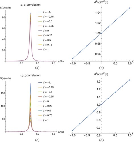
On the other hand, the correlations between longitudinal components have a much more dramatic effect on both the transition intensity and line width, with anti-correlated noise giving much sharper and more intense transitions. We can understand this in the following way. According to the Kubo-Anderson model, the spectral lineshape is determined by fluctuations in the transition frequency. In the anticorrelated case, the local fluctuations are perfectly synchronised but in opposite ways. That is, as the local site energy of one increases, the other site energy always decreases. Therefore, the two local fluctuations cancel each other out. In the fully correlated case, the fluctuations are also perfectly synchronised, but both site energies increase or decrease, which results in a broader spectral transition.

We next consider the effect of initial-state preparation on the quantum dynamics of the entangled qubits. For this, we introduce the following four Bell-states (18) $|{\mathrm{\Phi }}^{\pm }〉=\frac{1}{2}(|00〉\pm |11〉)$(18) (19) $|{\mathrm{\Psi }}^{\pm }〉=\frac{1}{2}(|01〉\pm |10〉)$(19) which correspond to the four maximally entangled quantum states of two qubits. From the previous discussion, longitudinal correlations appear to have the most profound effect on the dynamics, so we shall consider only that sort of coupling in this example.

The purity, $\gamma =\mathrm{tr}\left({\rho }^2\right)$, provides a useful measure of the degree to which a quantum state is mixed. Mathematically, $\gamma =1$ for a pure state since $\rho ={\rho }^2$ and takes a lower bound of $\gamma =1/4$ corresponding to the case where all 4 states of the system are equally probable. Initially, the system is in a pure state with $\gamma =1$ and evolves toward a mixed state as it evolves. At long time and low temperature, the system will relax completely to the ground state $|00〉$ with $\gamma =1$.

Figure 3(a,b) shows the purity of a composite $\mathrm{SU}\left(2\right)\otimes \mathrm{SU}\left(2\right)$ qubit pair vs time for systems prepared in a maximally entangled (Bell) state and subject to longitudinal (${\sigma }_z$) noise with various degrees of correlation or anti-correlation. In Figure 3(a), we take the initial state as a coherence between the doubly excited state $|11〉$ and the ground state $|00〉$, corresponding to the ${\mathrm{\Phi }}_{+}$ Bell state. Here, anticorrelation leads to a profound increase in the system's ability to retain its purity for nearly two orders of magnitude in time longer than the fully correlated case. In contrast, if the initial state is prepared in one of the ${\mathrm{\Psi }}_{\pm }$ Bell states, corresponding to a linear combination within the singly excited manifold of states, correlation enhances the system's ability to retain purity. The only difference between the two results are in the preparation of the initial state. This provides a potentially useful experimental means for determining the correlation or anti-correlation between local environments.

Figure 3. Purity(a,b) and fidelity (c,d) of composite $\mathrm{SU}\left(2\right)\otimes \mathrm{SU}\left(2\right)$ qubit pair vs time for systems prepared in a maximally entangled (Bell) state corresponding to (a,c)$|{\mathrm{\Phi }}^{+}〉$ or (b,d) ${\mathrm{\Psi }}^{+}$.

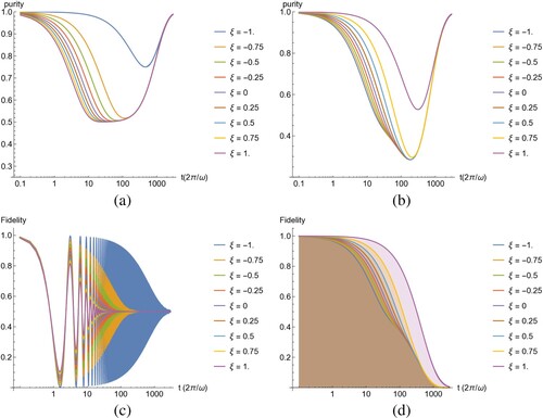
However, the fidelity (20) $F(\rho ,{\rho }^{\prime })={\left(\mathrm{tr}\left(\sqrt{\sqrt{\rho }{\rho }^{\prime }\sqrt{\rho }}\right)\right)}^2$(20) is also an important consideration for whether or not a given Bell state is suitable for an shared key. Fidelity provides a measure of the ‘closeness’ of two quantum states. It expresses the probability that one state will pass a test to identify itself as the other. By symmetry, $F(\rho ,\sigma )=F(\sigma ,\rho )$. In Figure 3(c,d), we compute the time-evolved fidelity $F({\rho }_0,{\rho }_t)$ starting from the ${\mathrm{\Phi }}^{+}$(c) or ${\mathrm{\Psi }}^{+}$(d) Bell states, versus various degrees of correlation between the baths. For ${\mathrm{\Phi }}^{+}$, the system loses fidelity rapidly and undergoes Rabi oscillation within the double excitation manifold spanned by ${\mathrm{\Phi }}^{+}$ and ${\mathrm{\Phi }}^{-}$. The fidelity eventually relaxes to $F=1/2$ for a long time, corresponding to complete relaxation into the ground state $|00〉$. As with purity, the envelope of fidelity is enhanced by anti-correlated noise.

In contrast, the correlated noise helps to maintain both the purity and fidelity of the ${\mathrm{\Psi }}^{+}$ Bell state. This state is an eigenstate of the bare system Hamiltonian can be prepared by direct photoexcitation from the ground state. Curiously, the above results suggest that correlated noise suppresses the optical response. However, the optical response is a measure of the coherence between the ground state and ${\mathrm{\Psi }}^{+}$ and not a measure of the purity or fidelity of a given state. While we focus on purity and fidelity, one can easily extend the results and approach for computing the coherence between the two spins, entanglement entropy, and similar measures of quantum entanglement.

We can straightforwardly understand these results by considering that in the correlated case, the local energy gaps are being modulated in the same way. In essence, if energy gap 1 increases then energy gap 2 is also likely to increase and vice verse if the two are correlated ($\xi >0$). This means that any entanglement that is sensitive to the sum of the two energies will experience a greater degree of environmental noise. Consequently, since the ${\mathrm{\Phi }}^{\pm }$ state corresponds to a superposition of the $|00〉$ ground state and $|11〉$ doubly excited state is expected to be more sensitive to correlated noise than anti-correlated noise. On the other hand, it should be insensitive to anti-correlated noise since the two gaps are increasing and decreasing in opposite ways on average. Similarly, the other two Bell states represent the tunnelling exchange between $|01〉$ and $|10〉$ and will be more sensitive to anti-correlated noise ($\xi <0$) since it leads to a greater average energetic mismatch between the two spins. On the other hand, it is less sensitive to correlated noise since both energy gaps are increasing and decreasing the same way on average.

3. Discussion

In this paper, we explored the role of noise correlation on a model open quantum system consisting of one and two coupled $\mathrm{SU}\left(2\right)$ qubits and showed how the dynamics and spectroscopy of the system can be profoundly affected by environmental correlations. This has deep implications for searching materials suitable for quantum communications and computation applications in which long coherence times and retention of are required. In the case of super-dense coding, a sender (A) and a receiver (B) can communicate several classical bits of information by only transmitting a smaller number of qubits, provided that A and B share an entangled resource [16]. Since this resource is subject to environmental noise, the ability of A and B to perform super-dense coding hinges on their ability to maintain the fidelity of the state of the shared resource. Similarly, quantum teleportation requires the sender and receiver to share a maximally entangled state [17]. Our results suggest that by knowing whether the state is subject to correlated or anticorrelated noise, A and B can be ensured that their shared resource state can maintain its purity long enough for the information to be communicated. We also suggest that the local noise correlation can be tuned by manipulating the local environment around the two qubits and that the approach can be extended for multiple spin-qubit systems. Indeed, it has been suggested that physical processes such as photosynthetic light-harvesting [18] and charge-separation in organic photovoltaics [19] may take advantage of environmental noise correlation in which the system acts much like a quantum heat engine [20,21].

Author Contributions

Eric Bittner: Supervision, Funding acquisition, Conceptualisation, Methodology, Formal analysis, Validation, Writing; Hao Li: Formal analysis, Methodology, Validation; Syad A Shah: Conceptualisation; Carlos Silva: Conceptualisation Funding acquisition; Andrei Piryatinski: Conceptualisation, Validation, Funding acquisition. All authors contributed to the final draft and editing of this manuscript.

Disclosure statement

No potential conflict of interest was reported by the author(s).

Data availability

Data supporting the findings of this study are available from the corresponding author on a reasonable request.

Additional information

Funding

The work at the University of Houston funded by the National Science Foundation (CHE-2102506) and the Robert A. Welch Foundation (E-1337). The work at Los Alamos National Laboratory was funded by the Laboratory Directed Research and Development (LDRD) program, 20220047DR. The National Science Foundation (DMR-1904293) funded the work at Georgia Tech.

Appendix 1.

A brief review of the Anderson-Kubo model for spectral lineshapes

A simple theory for spectral line-shapes was developed independently by Anderson and Kubo (AK) in the 1950s as a way to understand spectral line-broadening in magnetic resonance experiments [1–4]. We briefly recap the model as it pertains to the discussion in our paper.

Within the model, the transition frequency $\omega \left(t\right)$ of a two-state system is modulated about its average by (unspecified) fluctuations in the environment with (A1) $H/\hslash =\omega \left(t\right)\hat{\sigma }\left(3\right)$(A1) where $\hat{\sigma }\left(i\right)$ is a Pauli matrix and $\omega \left(t\right)={\omega }_o+\mathrm{\delta \omega }\left(t\right)$ with (A2) $\mathrm{d}\mathrm{\delta \omega }\left(t\right)=-\mathrm{\gamma \delta \omega }\left(t\right)\mathrm{d}t+s\mathrm{d}W\left(t\right)$(A2) with $〈\mathrm{\delta \omega }\left(t\right)〉=0$ where $W\left(t\right)$ is a Wiener process with (A3) $〈\mathrm{\delta \omega }\left(t\right)\mathrm{\delta \omega }\left(0\right)〉=\frac{s^2}{2\gamma }{e}^{-\gamma \left|t\right|}.$(A3) We also define ${\mathrm{\Delta }}^2=\frac{s^2}{2\gamma }$ as the fluctuation amplitude (which is proportional to the temperature of the environment, and $1/\gamma ={\tau }_c$ as the correlation time for the environment.

It is straightforward, then, to show using time-dependent perturbation theory that the optical response of the system can be given as (A4) $S\left(t\right)=\frac{1}{\mathrm{i\hslash }}〈{\mu }_{01}\left(t\right){\mu }_{10}\left(0\right)\rho (-\mathrm{\infty })〉$(A4) were ${\mu }_{01}\left(t\right)$ is the matrix element coupling state 0 to 1 written in the Heisenberg representation with (A5) ${\mu }_{01}\left(t\right)=e^{-i{\int }_0^t\omega \left(\tau \right)\mathrm{d}\tau }{\mu }_{01}\left(0\right).$(A5) Thus, (A6) $S\left(t\right)=\frac{|{\mu }_{01}{|}^2}{\mathrm{i\hslash }}{e}^{\mathrm{i\omega t}}〈e^{-i{\int }_0^t\mathrm{\delta \omega }\left(\tau \right)\mathrm{d}\tau }〉,$(A6) where the angle brackets denote the ensemble average. The bracketed expression can be evaluated using the cumulant expansion technique (A7) $〈e^{-i{\int }_0^t\mathrm{\delta \omega }\left(\tau \right)\mathrm{d}\tau }〉=e^{-g\left(t\right)}$(A7) (A8) $=1-g\left(t\right)+\frac{1}{2}{g}^2\left(t\right)+\cdots$(A8) and we expand $g\left(t\right)$ in terms of powers of $\mathrm{\delta \omega }\left(t\right)$ (A9) $g\left(t\right)=g_1\left(t\right)+g_2\left(t\right)+\cdots$(A9) where each $g_n$ is on the order of ${\mathcal{O}}^n\left(\mathrm{\delta \omega }\right)$. Since $g_1\left(t\right)=〈\mathrm{\delta \omega }\left(t\right)〉=0$ and all terms with n > 2 vanish under the Ito identity, only the $g_2$ term contributes to the cumulant summation. Thus, we obtain (A10) $g\left(t\right)=g_2\left(t\right)=\frac{1}{2}{\int }_0^t{\int }_0^t\mathrm{d}\tau \mathrm{d}{\tau }^{\prime }〈\mathrm{\delta \omega }\left({\tau }^{\prime }\right)\mathrm{\delta \omega }\left(\tau \right)〉.$(A10) Finally, since we assume the fluctuations are about a stationary value, the correlation function can only depend on the time interval $\tau -{\tau }^{\prime }$ so that (A11) $〈\mathrm{\delta \omega }\left({\tau }^{\prime }\right)\mathrm{\delta \omega }\left(\tau \right)〉=〈\mathrm{\delta \omega }({\tau }^{\prime }-\tau )\mathrm{\delta \omega }\left(0\right)={\mathrm{\Delta }}^2{e}^{-|{\tau }^{\prime }-\tau |/{\tau }_c}$(A11) where ${\mathrm{\Delta }}^2=\frac{{\sigma }^2}{2\gamma }$ and ${\tau }_c=1/\gamma$ is the correlation time as given above. Performing the double-time integration, (A12) $g\left(t\right)={\mathrm{\Delta }}^2{\tau }_c^2[e^{-t/{\tau }_c}+\frac{t}{{\tau }_c}-1]$(A12) which is the Kubo-lineshape function.

There are two important limits to this model. First, in which $\mathrm{\Delta }{\tau }_c\ll 1$ corresponds to the case of fast modulation. This results in a purely Lorentzian spectral line shape and a pure dephasing time of $T_2=({\mathrm{\Delta }}^2{\tau }_c{)}^{-1}$. Similarly, $\mathrm{\Delta }{\tau }_c\gg 1$ represents a slow modulation regime. Here, the spectral lineshape takes a purely Gaussian form, reflecting the inhomogeneities of the environment. Note that we recently extended this approach to account for non-stationary/non-equilibrium environments encountered in semiconducting systems [22,23].

Appendix 2.

Correlations amongst random variables

The Ornstein-Uhlenbeck process is a very useful method to account for many Markovian stochastic processes. Its multivariate representation is even more practical for physical processes. Here we discuss the multivariate Ornstein-Uhlenbeck process, including correlated Wiener processes, for the purpose of tackling realistic physical problems such as chromorphores coupled to their respective phonon environments but interacting with a common bath.

We write the multivariate Ornstein-Uhlenbeck process as a vector $\mathit{E}\left(t\right)$ composed of individual processes $X_i\left(t\right)$. The stochastic differential equation reads (A13) $\mathrm{d}\mathit{E}\left(t\right)=A[\mathit{\mu }-\mathit{E}(t\left)\right]\mathrm{d}t+B\mathrm{d}\mathit{W}\left(t\right),$(A13) in which A and B are coefficient matrices, $\mathit{\mu }$ is the vector of the Wiener process drift ${\mu }_i$ corresponding to $W_i$. $\mathit{W}\left(t\right)$ is the vector of Wiener processes $W_i\left(t\right)$ which are correlated through the correlation matrix (A14) $\xi (t,t^{\prime })\equiv {\delta }_{t{t}^{\prime }}\mathrm{d}\mathit{W}\left(t\right)\mathrm{d}\mathit{W}(t^{\prime }{)}^{\mathrm{T}}/\mathrm{d}t,$(A14) where the angular brackets represent the ensemble average. The matrix elements ${\xi }_{\mathrm{ij}}=\mathrm{d}{W}_i\left(t\right)\mathrm{d}{W}_j\left(t\right)/\mathrm{d}t$ are defined through the Itô isometry in higher dimensions. Obviously ${\xi }_{\mathrm{ii}}=1$ according to the quadratic variation $(\mathrm{d}{W}_t{)}^2=\mathrm{d}t$. ${\xi }_{\mathrm{ij}}$ varies from -1 to 1, respectively, corresponding to the fully anticorrelated and fully correlated cases. ${\xi }_{\mathrm{ij}}=0$ means that the two Wiener processes are completely uncorrelated.

According to the Itô's lemma, one finds the solution (A15) $\mathit{E}\left(t\right)=e^{-\mathrm{At}}\mathit{E}\left(0\right)+(1-e^{-\mathrm{At}})\mathit{\mu }+{\int }_0^t{e}^{-A(t-t^{\prime })}B\mathrm{d}\mathit{W}\left(t^{\prime }\right),$(A15) where $\mathit{E}\left(0\right)$ is the initial condition of the process $\mathit{E}\left(t\right)$, the mean value (A16) $〈\mathit{E}\left(t\right)〉=e^{-\mathrm{At}}〈\mathit{E}\left(0\right)〉+(1-e^{-\mathrm{At}})\mathit{\mu },$(A16) and the correlation function (A17) $\begin{array}{rl}〈\mathit{E}\left(t\right),{\mathit{E}}^{\mathrm{T}}\left(s\right)〉& \equiv 〈\left[\mathit{E}\right(t)-〈\mathit{E}(t)〉]{\left[\mathit{E}\right(s)-〈\mathit{E}(s)〉]}^{\mathrm{T}}〉\\ & =e^{-\mathrm{At}}〈\mathit{E}\left(0\right),{\mathit{E}}^{\mathrm{T}}\left(0\right)〉e^{-A^{\mathrm{T}}s}+{\int }_0^{min(s,t)}{e}^{-A(t-t^{\prime })}\mathrm{B\xi }{B}^{\mathrm{T}}{e}^{-A^{\mathrm{T}}(s-t^{\prime })}\mathrm{d}{t}^{\prime }\end{array}$(A17) following the Itô isometry in higher dimensions.

If $A{A}^{\mathrm{T}}=A^{\mathrm{T}}A$, one can find a unitary matrix S to diagonalise the coefficient matrix $\mathrm{SA}{S}^{†}=S{A}^{\mathrm{T}}{S}^{†}=\mathrm{diag}({\gamma }_1,{\gamma }_2,\dots ,{\gamma }_n)$. For deterministic initial condition $〈\mathit{E}\left(0\right),{\mathit{E}}^{\mathrm{T}}\left(0\right)〉=0$, so does the correlation function $〈\mathit{E}\left(t\right),{\mathit{E}}^{\mathrm{T}}\left(s\right)〉=S^{†}G(t,s)S$, in which (A18) $\begin{array}{rl}{\left[G\right(t,s\left)\right]}_{\mathrm{ij}}& =\frac{{\left(\mathrm{B\xi }{B}^{\mathrm{T}}\right)}_{\mathrm{ij}}}{{\gamma }_i+{\gamma }_j}[e^{-{\gamma }_i|t-s|}-e^{-{\gamma }_{i}t-{\gamma }_{j}s}](t\ge s),\\ & {\left[G\right(t,s\left)\right]}_{\mathrm{ij}}=\frac{{\left(\mathrm{B\xi }{B}^{\mathrm{T}}\right)}_{\mathrm{ij}}}{{\gamma }_i+{\gamma }_j}[e^{-{\gamma }_j|t-s|}-e^{-{\gamma }_{i}t-{\gamma }_{j}s}](t\le s).\end{array}$(A18) If the real parts of all A's eigenvalues are positive, one finds the stationary solution (A19) ${\mathit{E}}_{\mathrm{s}}\left(t\right)=\mathit{\mu }+{\int }_{-\mathrm{\infty }}^t{e}^{-A(t-t^{\prime })}B\mathrm{d}\mathit{W}\left(t^{\prime }\right),$(A19) with the stationary correlation matrix (A20) $〈{\mathit{E}}_{\mathrm{s}}\left(t\right),{\mathit{E}}_{\mathrm{s}}^{\mathrm{T}}\left(t^{\prime }\right)〉={\int }_{-\mathrm{\infty }}^{min(t^{\prime },t)}{e}^{-A(t-\tau )}\mathrm{B\xi }{B}^{\mathrm{T}}{e}^{-A^{\mathrm{T}}(t^{\prime }-\tau )}\mathrm{d}\tau$(A20) We define the stationary covariance matrix (A21) $\mathrm{\Sigma }=〈{\mathit{E}}_{\mathrm{s}}\left(t\right),{\mathit{E}}_{\mathrm{s}}^{\mathrm{T}}\left(t\right)〉,$(A21) then find a useful algebraic equation for stationary covariance matrix (A22) $\mathrm{A\sigma }+\sigma A^{\mathrm{T}}=\mathrm{B\xi }{B}^{\mathrm{T}}.$(A22) For s < t the stationary correlation function Equation (A20(A21) $\mathrm{\Sigma }=〈{\mathit{E}}_{\mathrm{s}}\left(t\right),{\mathit{E}}_{\mathrm{s}}^{\mathrm{T}}\left(t\right)〉,$(A21) ) can be written as (A23) $\begin{array}{rl}〈{\mathit{E}}_{\mathrm{s}}\left(t\right),{\mathit{E}}_{\mathrm{s}}^{\mathrm{T}}\left(s\right)〉& =e^{-A(t-s)}{\int }_{-\mathrm{\infty }}^s{e}^{-A(s-t^{\prime })}\mathrm{B\xi }{B}^{\mathrm{T}}{e}^{-A^{\mathrm{T}}(s-t^{\prime })}\mathrm{d}{t}^{\prime }\\ & =e^{-A(t-s)}\sigma s<t,\end{array}$(A23) and (A24) $=\sigma e^{-A^{\mathrm{T}}(s-t)}s>t.$(A24) The correlation function only depends on the time difference $|t-s|$ as expected for the stationary solution. We define the stationary correlation matrix $G_{\mathrm{s}}\left(\tau \right)=〈{\mathit{E}}_{\mathrm{s}}\left(t\right),{\mathit{E}}_{\mathrm{s}}^{\mathrm{T}}(t-\tau )〉$, obviously $G_{\mathrm{s}}\left(0\right)=\sigma$. Then the above relation can be written in the form of the regression theorem (A25) $\frac{\mathrm{d}}{\mathrm{d}\tau }\left[G_{\mathrm{s}}\right(\tau \left)\right]=\frac{\mathrm{d}}{\mathrm{d}\tau }〈{\mathit{E}}_{\mathrm{s}}\left(\tau \right),{\mathit{E}}_{\mathrm{s}}^{\mathrm{T}}\left(0\right)〉=-A{G}_{\mathrm{s}}\left(\tau \right).$(A25) Noting that $G_{\mathrm{s}}\left(0\right)=\sigma$, one can compute the stationary correlation matrix.

Since ${\sigma }^{\mathrm{T}}=\sigma$, we have (A26) $G_{\mathrm{s}}\left(\tau \right)={\left[G_{\mathrm{s}}\right(-\tau \left)\right]}^{\mathrm{T}}.$(A26) Therefore, one can find the spectrum matrix as the Fourier transform of the autocorrelation matrix $G_{\mathrm{s}}\left(\tau \right)$ (A27) $\begin{array}{rl}J\left(\omega \right)& =\frac{1}{2\pi }{\int }_{-\mathrm{\infty }}^{\mathrm{\infty }}{e}^{-\mathrm{i\omega \tau }}{G}_{\mathrm{s}}\left(\tau \right)\mathrm{d}\tau \\ & =\frac{1}{2\pi }{(A+\mathrm{i\omega })}^{-1}\mathrm{B\xi }{B}^{\mathrm{T}}{(A-\mathrm{i\omega })}^{-1}.\end{array}$(A27) As an example, we consider the case of the case of two correlated modes, in which we define the 2D Ornstein-Uhlenbeck process sby the SDEs $\begin{array}{rl}\mathrm{d}{E}_1\left(t\right)& =-{\gamma }_1{E}_1\left(t\right)\mathrm{d}t+s_{11}\mathrm{d}{B}_1\left(t\right)+s_{12}\mathrm{d}{B}_2\left(t\right),\\ \mathrm{d}{E}_2\left(t\right)& =-{\gamma }_2{E}_2\left(t\right)\mathrm{d}t+s_{21}\mathrm{d}{B}_1\left(t\right)+s_{22}\mathrm{d}{B}_2\left(t\right).\end{array}$The two Wiener processes $B_1\left(t\right)$ and $B_2\left(t\right)$ are coupled through the correlation parameter $\xi =\mathrm{d}{B}_1\left(t\right)\mathrm{d}{B}_2\left(t\right)/\mathrm{d}t$. The range of ξ is between $-1$ to 1 corresponding to the cases of complete anti-correlation and correlation, respectively. $\xi =0$ means that the two Wiener processes are completely decoupled. The solutions of the OU processes are $\begin{array}{rl}{E}_1\left(t\right)& =e^{-{\gamma }_{1}t}{E}_1\left(0\right)+s_{11}{\int }_0^t{e}^{-{\gamma }_1(t-s)}\mathrm{d}{B}_1\left(s\right)+s_{12}{\int }_0^t{e}^{-{\gamma }_1(t-s)}\mathrm{d}{B}_2\left(s\right),\\ E_2\left(t\right)& =e^{-{\gamma }_{2}t}{E}_2\left(0\right)+s_{21}{\int }_0^t{e}^{-{\gamma }_2(t-s)}\mathrm{d}{B}_1\left(s\right)+s_{22}{\int }_0^t{e}^{-{\gamma }_2(t-s)}\mathrm{d}{B}_2\left(s\right).\end{array}$From this we compute the mean values $\begin{array}{r}〈E_1\left(t\right)〉=〈E_1\left(0\right)〉e^{-{\gamma }_{1}t},\\ 〈E_2\left(t\right)〉=〈E_2\left(0\right)〉e^{-{\gamma }_{2}t},\end{array}$as well as the correlation functions $\begin{array}{rl}\mathrm{Cov}\left[E_1\right(t),E_1(s\left)\right]& =〈E_1(0{)}^2〉e^{-{\gamma }_1(t+s)}+\frac{s_{11}^2+s_{12}^2+2\xi s_{11}{s}_{12}}{2{\gamma }_1}[e^{-{\gamma }_1|t-s|}-e^{-{\gamma }_1(t+s)}],\\ \mathrm{Cov}\left[E_2\right(t),E_2(s\left)\right]& =〈E_2(0{)}^2〉e^{-{\gamma }_2(t+s)}+\frac{s_{21}^2+s_{22}^2+2\xi s_{21}{s}_{22}}{2{\gamma }_2}[e^{-{\gamma }_2|t-s|}-e^{-{\gamma }_2(t+s)}],\\ \mathrm{Cov}\left[E_1\right(t),E_2(s\left)\right]& =〈E_1\left(0\right),E_2\left(0\right)〉e^{-{\gamma }_{1}t-{\gamma }_{2}s}+\frac{s_{11}{s}_{21}+s_{12}{s}_{22}+\xi s_{11}{s}_{22}+\xi s_{12}{s}_{21}}{{\gamma }_1+{\gamma }_2}{e}^{-{\gamma }_{1}t-{\gamma }_{2}s}\\ & [e^{({\gamma }_1+{\gamma }_2)min(s,t)}-1],\\ \mathrm{Cov}\left[E_2\right(t),E_1(s\left)\right]& =〈E_1\left(0\right),E_2\left(0\right)〉e^{-{\gamma }_{2}t-{\gamma }_{1}s}+\frac{s_{11}{s}_{21}+s_{12}{s}_{22}+\xi s_{11}{s}_{22}+\xi s_{12}{s}_{21}}{{\gamma }_1+{\gamma }_2}{e}^{-{\gamma }_{2}t-{\gamma }_{1}s}\\ & [e^{({\gamma }_1+{\gamma }_2)min(s,t)}-1].\end{array}$Using these we find the spectral density matrix for the correlated processes as (A28) $J\left(\omega \right)=\frac{1}{2\pi }\left[\begin{array}{cc}\frac{s_{11}^2+2\xi s_{11}{s}_{22}+s_{12}^2}{{\gamma }_1^2+{\omega }^2}& \frac{s_{12}{s}_{22}+s_{11}{s}_{21}+\xi (s_{12}{s}_{21}+s_{11}{s}_{22})}{({\gamma }_1+\mathrm{i\omega })({\gamma }_2-\mathrm{i\omega })}\\ \frac{s_{12}{s}_{22}+s_{11}{s}_{21}+\xi (s_{12}{s}_{21}+s_{11}{s}_{22})}{({\gamma }_1-\mathrm{i\omega })({\gamma }_2+\mathrm{i\omega })}& \frac{s_{11}^2+2\xi s_{21}{s}_{22}+s_{22}^2}{{\gamma }_2^2+{\omega }^2}\end{array}\right].$(A28)

Appendix 3.

Redfield tensor elements for cross correlation between x and z for a single $\mathit{SU}\left(2\right)$ qubit

The Bloch-Redfield equations give the quantum dynamics of the reduced density matrix according to (A29) $d_t{\rho }_{\alpha {\alpha }^{\prime }}=-i({\omega }_{\alpha }-{\omega }_{\alpha }^{\prime }){\rho }_{\alpha {\alpha }^{\prime }}-\sum _{\text{β}{\text{β}}^{\prime }}{\mathcal{R}}_{\alpha {\alpha }^{\prime };\text{β}{\text{β}}^{\prime }}({\rho }_{\text{β}{\text{β}}^{\prime }}-{\rho }_{\text{β}{\text{β}}^{\prime }}^{\mathrm{eq}})$(A29) where ${\rho }^{\mathrm{eq}}$ is the equilibrium reduced density matrix and $\mathcal{R}$ is the Bloch-Redfield tensor with elements [12–15] (A30) $\begin{array}{rl}{\mathcal{R}}_{\alpha {\alpha }^{\prime };\text{β}{\text{β}}^{\prime }}& =\sum _{\mathrm{nm}}\left\{{\delta }_{{\alpha }^{\prime }{\text{β}}^{\prime }}\sum _{\gamma }{J}_{\mathrm{nm}}\right({\omega }_{\text{β}}-{\omega }_{\gamma }\left)\right(A_n{)}_{\gamma \text{β}}(A_m{)}_{\mathrm{\alpha \gamma }}\\ & -\left(J_{\mathrm{nm}}\right({\omega }_{\alpha }^{\prime }-{\omega }_{\text{β}}^{\prime })+J_{\mathrm{nm}}({\omega }_{\text{β}}-{\omega }_{\alpha }\left)\right)\left(A_n{)}_{{\text{β}}^{\prime }{\alpha }^{\prime }}\right(A_m{)}_{\alpha \text{β}}\\ & +{\delta }_{\alpha \text{β}}\sum _{\gamma }{J}_{\mathrm{nm}}({\omega }_{\gamma }-{\omega }_{\text{β}}^{\prime })\left(A_n{)}_{{\text{β}}^{\prime }\gamma }\right(A_m{)}_{\gamma {\alpha }^{\prime }}\}\end{array}$(A30) where $(A_n{)}_{\alpha \text{β}}=〈\alpha |{\hat{A}}_n|\text{β}〉$ are the matrix elements of the ${\hat{A}}_n$ operator in the eigenbasis of $H_o$ and $J_{\mathrm{nm}}\left(\omega \right)$ are elements of the generalised spectral matrix characterising the coupling between the system and its environment. Table A1 gives the tensor elements for the case of a single qubit with transition frequency ϵ coupled to a noisy environment through both longitudinal (through ${\hat{\sigma }}_z$) and transverse (through ${\hat{\sigma }}_x$ or ${\hat{\sigma }}_y$). $J_{\mathrm{ij}}\left(\omega \right)$ to denote the spectral density associated with the correlation function $〈E_i\left(t\right)E_j\left(t^{\prime }\right)〉$.

The second column indicates whether or not $R_{\mathrm{ijkl}}$ is non-vanishing within the secular approximation. (A31) $R_{\mathrm{ij};\mathrm{kl}}^{\sec }=({\delta }_{\mathrm{ij}}{\delta }_{\mathrm{kl}}+{\delta }_{\mathrm{ik}}{\delta }_{\mathrm{jl}}(1-{\delta }_{\mathrm{ij}}{\delta }_{\mathrm{kl}}\left)\right)R_{\mathrm{ij};\mathrm{kl}}$(A31) When operating under this limit, the system populations are decoupled from the coherences, following a regular Pauli Master equation with the population rate matrix $R_{\mathrm{iikk}}$. This ensures population conservation and achieves the correct thermal equilibrium over extended periods. Under this approximation, the density matrix exhibits the appropriate physical behaviour with $\mathrm{Tr}\left[\rho \right]=1$. The population rate matrix, being real, facilitates exponential relaxation of the populations. Coherences are also fully separated from the population and experience attenuation by the dephasing rates $R_{\mathrm{ij};\mathrm{ij}}$. Generally, $R_{\mathrm{ij};\mathrm{ij}}$ is complex, with its imaginary component representing bath-induced energy shifts. For example, under the secular approximation, we expect that $R_{11;11}+R_{22;11}=R_{22;22}+R_{11;22}=0$ and $R_{12;12}=R_{21;21}^{\ast }$ for the coherence terms. The presence of the cross-correlation terms does not lead to a violation of these conditions.

Table A1. Redfield tensor elements for $\mathrm{SU}\left(2\right)$ qubit with cross-correlation between ${\hat{\sigma }}^x$ and ${\hat{\sigma }}^z$ noise terms.

i	j	k	l	Secular	${\mathcal{R}}_{\mathrm{ij};\mathrm{kl}}$	Ornstein-Uhlenbeck
1	1	1	1	Secular	$J_{\mathrm{xx}}(-ϵ)+J_{\mathrm{xx}}\left(ϵ\right)$	$\frac{2s_x(s_x+2\xi s_{\mathrm{xz}})}{{\gamma }_x^2+{ϵ}^2}$
1	1	1	2	Non-Secular	$-J_{\mathrm{xz}}\left(0\right)-J_{\mathrm{zx}}\left(0\right)$	$-\frac{2(s_x(s_{\mathrm{xz}}+\xi s_z)+\xi s_{\mathrm{xz}}^2)}{{\gamma }_x{\gamma }_z}$
1	1	2	1	Non-Secular	$J_{\mathrm{xz}}(-ϵ)-J_{\mathrm{zx}}(-ϵ)-2J_{\mathrm{zx}}\left(0\right)$	$-\frac{2({\gamma }_x^2(\mathrm{iϵ}{\gamma }_z+{\gamma }_z^2+{ϵ}^2)-\mathrm{iϵ}{\gamma }_x{\gamma }_z^2+{ϵ}^2({\gamma }_z^2+{ϵ}^2))(s_x(s_{\mathrm{xz}}+\xi s_z)+\xi s_{\mathrm{xz}}^2)}{{\gamma }_x{\gamma }_z({\gamma }_x^2+{ϵ}^2)({\gamma }_z^2+{ϵ}^2)}$
1	1	2	2	Secular	$-J_{\mathrm{xx}}(-ϵ)-J_{\mathrm{xx}}\left(ϵ\right)$	$-\frac{2s_x(s_x+2\xi s_{\mathrm{xz}})}{{\gamma }_x^2+{ϵ}^2}$
1	2	1	1	Non-Secular	$-2J_{\mathrm{xz}}(-ϵ)-J_{\mathrm{xz}}\left(0\right)+J_{\mathrm{zx}}\left(0\right)$	$-\frac{2(s_x(s_{\mathrm{xz}}+\xi s_z)+\xi s_{\mathrm{xz}}^2)}{(ϵ+i{\gamma }_x)(ϵ-i{\gamma }_z)}$
1	2	1	2	Secular	$2\left(J_{\mathrm{xx}}\right(ϵ)+2J_{\mathrm{zz}}(0\left)\right)$	$\frac{4s_{\mathrm{xz}}^2({\gamma }_x^2+{ϵ}^2)+4\xi s_{\mathrm{xz}}(2s_z({\gamma }_x^2+{ϵ}^2)+s_x{\gamma }_z^2)+2s_x^2{\gamma }_z^2}{{\gamma }_z^2({\gamma }_x^2+{ϵ}^2)}$
1	2	2	1	Non-Secular	$-2J_{\mathrm{xx}}(-ϵ)$	$-\frac{2s_x(s_x+2\xi s_{\mathrm{xz}})}{{\gamma }_x^2+{ϵ}^2}$
1	2	2	2	Non-Secular	$J_{\mathrm{xz}}(-ϵ)+J_{\mathrm{zx}}(-ϵ)$	$\frac{2({\gamma }_x{\gamma }_z+{ϵ}^2)(s_x(s_{\mathrm{xz}}+\xi s_z)+\xi s_{\mathrm{xz}}^2)}{({\gamma }_x^2+{ϵ}^2)({\gamma }_z^2+{ϵ}^2)}$
2	1	1	1	Non-Secular	$-J_{\mathrm{xz}}\left(ϵ\right)-J_{\mathrm{zx}}\left(ϵ\right)$	$-\frac{2({\gamma }_x{\gamma }_z+{ϵ}^2)(s_x(s_{\mathrm{xz}}+\xi s_z)+\xi s_{\mathrm{xz}}^2)}{({\gamma }_x^2+{ϵ}^2)({\gamma }_z^2+{ϵ}^2)}$
2	1	1	2	Non-Secular	$-2J_{\mathrm{xx}}\left(ϵ\right)$	$-\frac{2s_x(s_x+2\xi s_{\mathrm{xz}})}{{\gamma }_x^2+{ϵ}^2}$
2	1	2	1	Secular	$2\left(J_{\mathrm{xx}}\right(-ϵ)+2J_{\mathrm{zz}}(0\left)\right)$	$\frac{4s_{\mathrm{xz}}^2({\gamma }_x^2+{ϵ}^2)+4\xi s_{\mathrm{xz}}(2s_z({\gamma }_x^2+{ϵ}^2)+s_x{\gamma }_z^2)+2s_x^2{\gamma }_z^2}{{\gamma }_z^2({\gamma }_x^2+{ϵ}^2)}$
2	1	2	2	Non-Secular	$2J_{\mathrm{xz}}\left(ϵ\right)+J_{\mathrm{xz}}\left(0\right)-J_{\mathrm{zx}}\left(0\right)$	$\frac{2(s_x(s_{\mathrm{xz}}+\xi s_z)+\xi s_{\mathrm{xz}}^2)}{(ϵ-i{\gamma }_x)(ϵ+i{\gamma }_z)}$
2	2	1	1	Secular	$-J_{\mathrm{xx}}(-ϵ)-J_{\mathrm{xx}}\left(ϵ\right)$	$-\frac{2s_x(s_x+2\xi s_{\mathrm{xz}})}{{\gamma }_x^2+{ϵ}^2}$
2	2	1	2	Non-Secular	$-J_{\mathrm{xz}}\left(ϵ\right)+J_{\mathrm{zx}}\left(ϵ\right)+2J_{\mathrm{zx}}\left(0\right)$	$\frac{2({\gamma }_x^2(-\mathrm{iϵ}{\gamma }_z+{\gamma }_z^2+{ϵ}^2)+\mathrm{iϵ}{\gamma }_x{\gamma }_z^2+{ϵ}^2({\gamma }_z^2+{ϵ}^2))(s_x(s_{\mathrm{xz}}+\xi s_z)+\xi s_{\mathrm{xz}}^2)}{{\gamma }_x{\gamma }_z({\gamma }_x^2+{ϵ}^2)({\gamma }_z^2+{ϵ}^2)}$
2	2	2	1	Non-Secular	$J_{\mathrm{xz}}\left(0\right)+J_{\mathrm{zx}}\left(0\right)$	$\frac{2(s_x(s_{\mathrm{xz}}+\xi s_z)+\xi s_{\mathrm{xz}}^2)}{{\gamma }_x{\gamma }_z}$
2	2	2	2	Secular	$J_{\mathrm{xx}}(-ϵ)+J_{\mathrm{xx}}\left(ϵ\right)$	$\frac{2s_x(s_x+2\xi s_{\mathrm{xz}})}{{\gamma }_x^2+{ϵ}^2}$

Notes: The second column indicates whether the term survives under the secular approximation, which separates the evolution of the population and the coherence terms. The last column gives the tensor element within the correlated Ornstein-Uhlenbeck model.

References

- R. Kubo, Note on the stochastic theory of resonance absorption, J. Phys. Soc. Jpn 9 (1954), pp. 935–944. https://doi.org/10.1143/JPSJ.9.935.
- P.W. Anderson, A mathematical model for the narrowing of spectral lines by exchange or motion, J. Phys. Soc. Jpn 9 (1954), pp. 316–339. https://doi.org/10.1143/JPSJ.9.316.
- R. Kubo, A Stochastic Theory of Line Shape, in Advances in Chemical Physics, K.E. Shuler (Ed.), 1969, pp. 101–127.
- S. Mukamel, Stochastic theory of resonance Raman line shapes of polyatomic molecules in condensed phases, J. Chem. Phys. 82 (1984), pp. 5398–5408. https://doi.org/10.1063/1.448623.
- A.Y. Smirnov and M.H. Amin, Theory of open quantum dynamics with hybrid noise, New. J. Phys. 20 (2018), p. 103037.
- S. Golkar and M.K. Tavassoly, Dynamics of entanglement protection of two qubits using a driven laser field and detunings: Independent and common, markovian and/or non-markovian regimes, Chinese Phys. B 27 (2018), pp. 040303.
- J.-T. Hsiang, O. Arisoy, and B.-L. Hu, Entanglement dynamics of coupled quantum oscillators in independent nonmarkovian baths, Entropy 24(12) (2022), pp. 1814.
- Y. Li, J. Zhou, and H. Guo, Effect of the dipole-dipole interaction for two atoms with different couplings in a non-markovian environment, Phys. Rev. A 79 (2009), p. 012309.
- G. Mouloudakis and P. Lambropoulos, Coalescence of non-markovian dissipation, quantum zeno effect, and non-hermitian physics in a simple realistic quantum system, Phys. Rev. A. 106 (2022), pp. 053709.
- G. Mouloudakis and P. Lambropoulos, Entanglement instability in the interaction of two qubits with a common non-markovian environment, Quantum Information Processing 20 (2021), pp. 331.
- C. Gardner, Stochastic Methods-A Handbook for the Natural and Social Sciences, 4th ed., Springer Series in Synergetics, Springer, Berlin, Heidelberg, 2009.
- R. Konrat and H. Sterk, Cross-correlation effects in the transverse relaxation of multiple-quantum transitions of heteronuclear spin systems, Chem. Phys. Lett. 203 (1993), pp. 75–80.
- A.G. Redfield, On the theory of relaxation processes, IBM J. Res. Dev. 1 (1957), pp. 19–31.
- I. Solomon, Relaxation processes in a system of two spins, Phys. Rev. 99 (1955), pp. 559–565. cited by: 2808.
- P.N. Argyres and P.L. Kelley, Theory of spin resonance and relaxation, Phys. Rev. 134 (1964), pp. 98–111.
- C.H. Bennett and S.J. Wiesner, Communication via one- and two-particle operators on einstein-podolsky-rosen states, Phys. Rev. Lett. 69 (1992), pp. 2881–2884.
- C.H. Bennett, G. Brassard, C. Crépeau, R. Jozsa, A. Peres, and W.K. Wootters, Teleporting an unknown quantum state via dual classical and einstein-podolsky-rosen channels, Phys. Rev. Lett. 70 (1993), pp. 1895–1899.
- G.S. Engel, T.R. Calhoun, E.L. Read, T.-K. Ahn, T. Mančal, Y.-C. Cheng, R.E. Blankenship, and G.R. Fleming, Evidence for wavelike energy transfer through quantum coherence in photosynthetic systems, Nature 446 (2007), pp. 782–786.
- E.R. Bittner and C. Silva, Noise-induced quantum coherence drives photo-carrier generation dynamics at polymeric semiconductor heterojunctions, Nat. Commun. 5 (2014), p. 3119.
- K.E. Dorfman, D.V. Voronine, S. Mukamel, and M.O. Scully, Photosynthetic reaction center as a quantum heat engine, Proc. Nat. Acad. Sci. 110 (2013), pp. 2746–2751. REFDOI https://www.pnas.org/doi/pdf/10.1073/pnas.1212666110.
- M.O. Scully, K.R. Chapin, K.E. Dorfman, M.B. Kim, and A. Svidzinsky, Quantum heat engine power can be increased by noise-induced coherence, Proc. Nat. Acad. Sci. 108 (2011), pp. 15097–15100. REFDOI https://www.pnas.org/doi/pdf/10.1073/pnas.1110234108.
- H. Li, A.R. Srimath Kandada, C. Silva, and E.R. Bittner, Stochastic scattering theory for excitation-induced dephasing: Comparison to the Anderson–Kubo lineshape, J. Chem. Phys. 153 (2020), p. 154115. https://doi.org/10.1063/5.0026467.
- A.R. Srimath Kandada, H. Li, F. Thouin, E.R. Bittner, and C. Silva, Stochastic scattering theory for excitation-induced dephasing: Time-dependent nonlinear coherent exciton lineshapes, J. Chem. Phys. 153 (2020), p. 164706. https://doi.org/10.1063/5.0026351.