Parameter optimisation of the Eolic Cell to augment wind power density through the Metamodel of Optimal Prognosis

ABSTRACT

The present work advances a methodology to optimise variables involved in fluid dynamic phenomena for augmented wind turbines. Particularly, the study focuses on improving the performance of a convergent-divergent augmented wind turbine based on eolic cells designed to increase wind speed at the throat section, where a peripherally supported magnetic levitation rotor will be installed as part of a novel wind energy system for distributed generation. Previous studies focused on maximising average wind velocity as the target variable. In contrast, this study shifted its focus to power density, resulting in more effective and consistent results. Numerical axisymmetric computational fluid dynamics simulations were conducted to determine the impact of these improvements. Response surfaces were created for parametric analysis, and the metamodel of optimal prognosis was implemented to provide accuracy. The results indicate a significant improvement in available power, with an average increase of up to 12.5 times compared to non-augmented conditions.

KEYWORDS:

• Wind energy
• CFD simulation
• metamodel of optimal prognosis
• augmentation effect
• distributed generation

Highlights

• Eolic Cells significantly enhance the power augmentation effect by up to 12.5 times compared to non-augmented conditions.

• The use of average wind velocity as a measure of available power is inadequate due to its implicit oversimplification that assumes a linear wind velocity profile.

• Opting for available power as the target variable for optimisation is more suitable since it accounts for the impact of a nonlinear wind velocity profile.

• The introduction of modularity, to a certain extent, does not significantly compromise the power augmentation effect and the corresponding available power.

• On average, this research substantially improves the available power by 2.7 times when compared to a previous study on Eolic Cells.

Abbreviation table

Table

Abbreviation	Description
CDAWT	Convergent-Divergent Augmented Wind Turbine
ECs	Eolic Cells
CFD	Computational Fluid Dynamics
DAWT	Diffuser-Augmented Wind Turbines
RANS	Reynolds Averaged Navier-Stokes
DWT	Ducted Wind Turbine
MOP	Metamodel of Optimal Prognosis
SST	Shear-Stress Transport
GCI	Grid Convergence Index
IAC	Internal Aerodynamic Chamber
LHS	Latin Hypercube Sampling
L	Chord length
Ym	Throat diameter
Xm	Throat distance from inlet opening
RTO	Ratio of throat diameter over inlet opening diameter
P	Available power
AWV	Average wind velocity
COD	Coefficient of Determination
COI	Coefficient of Importance
COP	Coefficient of Prognosis
4dBZC	Fourth-degree Bezier Curves
Cs	Strain coefficient
WS	Wind speed
NLPQL	Nonlinear Programming by Quadratic Langrangian
Simplex	Downhill Simplex Method
MISQP	Mix Integer Sequential Quadratic Programming

I. Introduction

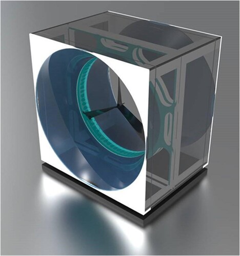
The current research aims to advance state-of-the-art methodologies to optimise variables involved in fluid dynamic phenomena and alternative approaches to wind energy systems for distributed generation. Specifically, this study applies a particular methodology to improve the performance of a new type of wind turbine design known as Convergent-Divergent Augmented Wind Turbine (CDAWT), based on the innovative concept of Eolic Cells (EC). These are individual, modular wind systems whose structures are designed to augment wind speed in the throat section, where a special wind turbine rotor is installed. The rotor transmits power to the periphery through a power transmission magnetic mechanism. This rotor type has a peripheral support that differs from the conventional central axis support. The advantage of this design is linked to eliminating turbulence generated by the presence of an electric generator coupled to the horizontal axis. This new wind energy system configuration seeks to maximise the power coefficient by augmenting the power density and reducing turbulence flow. Figure 1 shows a computational representation of an EC integrated with a peripherally supported wind turbine rotor.

Figure 1. Computational rendering of the Eolic Cell with an integrated peripherally supported wind turbine.

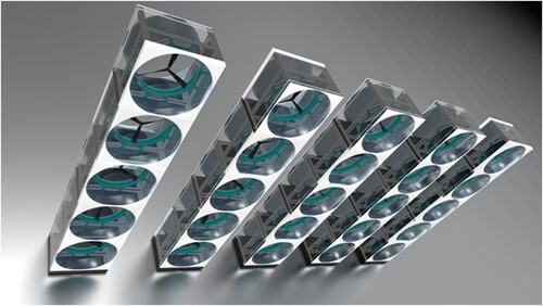
Figure 2 illustrates EC’s modularity by showcasing an array of ECs arranged in tower configurations.

Figure 2. Illustration of an organised collection of structures consisting of modular Eolic Cells.

It is important to highlight that this particular work is just one aspect of a comprehensive project that delves into studying EC components from various disciplines. Specifically, the present manuscript focuses on optimising the EC’s aerodynamic geometry to attain the highest possible power density. Subsequently, in future studies, the multidisciplinary project will address the analysis and optimisation of a new peripherally supported wind turbine in conjunction with the optimised EC’s geometry resulting from this study. The reason for this segmentation lies in the fact that both the EC’s geometry and EC’s peripherally supported wind turbine have distinct underlying performance parameters, in addition to differentiated target variables for optimisation. While the EC’s geometry aims to maximise power density, the EC’s wind turbine aims to maximise the power coefficient. Therefore, segmenting the study of an integrated system into subsystems simplifies the multidimensional complexity of the parametric analysis, reducing computational costs and increasing the effectiveness of the optimisation tools used. Furthermore, in general, carrying out the study of each subsystem in the above-indicated order (first the EC’s geometry optimisation and then EC’s wind turbine rotor) is relevant due to the significant impact that the geometry surrounding a wind turbine has on laminar flow and resulting wind profile, which undoubtedly affects wind turbine performance. In other words, optimising the wind turbine’s parameters without first characterising the new wind profile caused by the presence of a geometry surrounding the wind turbine is an imprecise and incomplete approach.

1.1. Focus of the studies on augmented wind turbines

Previous research in this field has explored various strategies to improve the efficiency of wind energy systems, from aerodynamic improvements in blades to innovations in system architecture. The trend of innovating over external geometries around wind turbines has led to considering the implementation of different shapes for ducts and diffusers designed to redirect and accelerate wind flow towards the wind turbine’s rotor (Hu and Cheng 2008). Although several designs have been proposed to augment vertical-axis wind turbines (Allaei and Andreopoulos 2014; Hang et al. 2018; Jadallah, Farag, and Hamdi 2018;; Salem, Mohammedredha, and Alawadhi 2023; Santoli et al. 2014 Wang et al. 2017; Wang et al. 2020; Wang et al. 2022; Wong et al. 2018), with the common goal of maximising wind energy harnessing, this work focuses only on research related to augmented horizontal-axis wind turbines.

In this research, numerous articles discuss Diffuser-Augmented Wind Turbines (DAWT) and their power coefficient enhancement through diffuser implementation. Nunes, Brasil Junior, and Oliveira (2020) conducted a meta-study that reviewed and categorised 155 research on DAWT into 16 specific topics, introducing a discussion on relevant parameters, main research branches, and their most important findings.

1.2. Theoretical contributions for wind turbines with diffusers

Lilley and Rainbird’s (1956) research was one of the first to evaluate wind turbine performance by implementing ducting and establishing a comparative concept of power coefficient between bare and augmented wind turbines. Other studies have contributed to the theoretical framework in this field by presenting simplified surrogate models (Foreman, Gilbert, and Oman 1978; Gilbert Barry, Oman Richard, and Foreman Kenneth 1978; Oman, Foreman, and Gilbert 1977) and one-dimensional theory analysis (de Vries 1979). These models require empirical parameters and experimental data to predict diffuser performance over different geometries and simulant situations. Jamieson’s (2008), (Jamieson 2009) and Van Bussel Gerard, van Bussel Dr Gerard, and Van Bussel Gerard’s (2007) analytical models introduced an advance in theory by showing the ability of DAWTs to overcome the Betz limit, which was later reinforced by Foote et al.’s research (Foote and Agarwal 2012). Afterward, new methods for numerically evaluating the performance of DAWTs were developed following the theoretical actuator disc models (Aranake and Duraisamy 2017; Dighe et al. 2019; Dighe, Avallone, and van Bussel 2016; Kumar and Saha 2019; Ohya et al. 2012; Sorribes-Palmer et al. 2017; Wang, Song, and Yan 2019).

1.3. Diffusers with aerodynamic profile

One common strategy for improving diffusers is to increase the outlet area by modifying the flange angle. However, these modifications can lead to boundary layer separation and decreased performance. Researchers suggest that using an aerodynamic diffuser instead of the usual conical diffuser can help avoid this problem, improving efficiency. Research by Fletcher Clive (1981) and Aranake Aniket, Lakshminarayan Vinod, and Karthik (2013; 2015) involved experimenting with various airfoils to achieve a target power coefficient. Meanwhile, Bagheri-Sadeghi, Helenbrook, and Visser (2021) analyzed the airfoil layout to determine the maximum power density. In contrast, Venters and Cols (Venters and Helenbrook 2013) and Civalier et al. (2011) conducted experiments to analyze the impact of airfoils on pressure distribution. Similarly, Mehmood et al. (Mehmood, Liang, and Khan 2012; Mehmood, Zhang, and Khan 2012) conducted studies to analyze the axial velocity distributions for different airfoils with augmented wind speed as the target variable.

1.4. Curved diffusers

Most DAWTs use a simplified curved shape to achieve airfoil-like results without disrupting the flow. However, some curved diffusers can create a recirculation zone on the outer surface (Dighe et al. 2018). This design concept can be applied in wind farms (Ohya and Karasudani 2010) and can facilitate optimisation methods by adjusting the position of the coordinates that control the shape of the diffuser curve (Amer et al. 2013; Foote and Agarwal 2012).

1.5. Influence of diffuser length

Another strategy for improving diffusers’ performance is to increase their length to achieve a higher area ratio between the diffuser and the rotor. This approach aims to prevent an increase in the expansion angle, which reduces the risk of boundary layer separation. Research has focused on analyzing the impact of varying the diffuser length while maintaining the diffuser’s shape and expansion angle. Matsushima, Takagi, and Muroyama (2006) and Ohya et al. (2006) found that increasing the diffuser length led to significant performance improvements up to an optimum length, beyond which marginal improvements were not substantial. Similarly, Ohya and Karasudani (Ohya et al. 2012), Buehrle, Kishore, and Priya (2013), and Shi et al. (2015) analyzed the influence of the ratio between diffuser length to turbine diameter, defining this ratio as a parameter to optimise diffuser design within a range of optimal values.

1.6. Research with optimisation methods

Optimisation methods such as evolutionary algorithms (Alpman 2018; Daniele, Ferrauto, and Coiro 2013;; Khamlaj and Rumpfkeil 2018; Leloudas et al. 2020 Oka et al. 2015; Rahmatian, Shahrbabaki, and Moeini 2023) and gradient-based optimisation processes (Calle, Baca, and Gorizales 2022) can be employed to achieve better diffuser designs. These methods are promising for their ability to be used with other computational analysis models and the convenience of analyzing many geometries without needing to manufacture each corresponding physical prototype. As a summary of different optimisation methods utilised in the field, Table 1 compares select research conducted on DAWTs over the past decade. These studies focus on improving diffuser performance to increase the power coefficient.

Table 1. Comparison of select research on DAWTs focusing on improving diffuser performance to increase the power coefficient.

Research reference	Daniele, Ferrauto, and Coiro (2013)	Khamlaj and Rumpfkeil (2018)	Leloudas et al. (2020)	Rahmatian, Shahrbabaki, and Moeini (2023)	Present Research
Publishing year	2015	2018	2019	2023	2024
Optimisation method	Non-dominated Sorting Genetic Algorithm (NSGA-II)	Multi-objective genetic algorithm (MOGA)	Asynchronous Parallel Differential Evolution Algorithm (DE)	Single-Objective Genetic Algorithm (SOGA)	Nonlinear Programming by Quadratic Langrangian (NLPQL), Downhill Simplex Method (Simplex), Mix Integer Sequential Quadratic Programming (MISQP)
Turbulence model	RANS Model of Spalart–Allmaras	RANS Standard k-epsilon	RANS Model Shear-Stress Transport	RANS Model Shear-Stress Transport	RANS Model Shear-Stress Transport
Variables of study	Pitch angle for the diffuser. Abscissa variation (Legendre polynomial). Upper surface ordinates. Lower surface ordinates.	Throat radius. Input radius. Diffuser radius. Flange height. Diffuser length. Inlet length.	Diffuser Length. Inlet Radius. Throat Radius. Exit Radius.	Nozzle length. Nozzle angle. Diffuser length. Diffuser angle. Flange length. Flange angle. Throat diameter.	Throat radius (Ym). Throat distance from inlet opening (Xm). Chord length (L). Inlet opening diameter. Outlet opening diameter.
Augmented geometry shape	Airfoil	Thin curve	Airfoil	Convergent-divergent geometry	Aerodynamic convergent – divergent geometry
Geometry parameterization	Legendre polynomial	Quadratic polynomial	Free-Form Deformation (FFD).	Straight lines	Fourth-degree Bezier curves.

The objective of the research conducted by Daniele et al. (Coiro, Daniele, and Della Vecchia 2016; Daniele and Coiro 2013; Daniele, Ferrauto, and Coiro 2013) is to optimise an aerodynamic diffuser by using the power coefficient obtained directly from the STAR CCM+ analysis solver. Similarly, Tariq et al. (Khamlaj and Rumpfkeil 2018) aim to optimise both duct and blade shape by using the power coefficient as the target function while minimising the drag and thrust coefficients calculated in OpenFOAM. Leloudas et al.’s research (Leloudas et al. 2020) maximises the average wind-speed increase and minimises drag within geometrical constraints. In contrast, Rahmatian et al.’s research (Rahmatian, Shahrbabaki, and Moeini 2023) aims to maximise the maximum wind velocity and the average wind velocity at the duct’s throat, where a wind turbine rotor is placed, in order to increase the power coefficient accordingly. In contrast to prior research, the present study focuses on optimising a convergent-divergent aerodynamic geometry without a pre-installed wind turbine rotor to facilitate an explicit wind profile characterisation with no external disturbance. The main objective is maximising the available power for a peripherally supported wind turbine to be installed at the throat section.

Regarding geometry parameterisation, surrogate models are applied to control the diffuser design for optimisation. Daniele, Ferrauto, and Coiro (2013) use an aerodynamic profile over which a shape optimisation process is performed by applying Legendre polynomials. Tariq et al. (Khamlaj and Rumpfkeil 2018) optimise a slender curve using a quadratic polynomial. Leloudas et al. (2020) apply the Free-Form Deformation (FFD) technique to optimise an airfoil geometry. Rahmatian, Shahrbabaki, and Moeini (2023) vary the angle and length of a duct’s convergent and divergent sections to find the optimal design of a straight-line airfoil. Conversely, the present study optimises a convergent-divergent geometry formed by a revolved aerodynamic airfoil parametrised using a fourth-degree Bézier curve, where the position of the Bezier-curve control points controls the EC’s aerodynamic geometry.

In contrast to comparative studies that utilise genetic algorithms, this research employs three gradient-based optimisation models, which deliver accurate results without requiring high computational capacity.

For turbulence modeling, both compared studies and the present study employ RANS-SST models, with the k - ω model applied to regions close to walls and the k − ϵ model used in regions away from walls. Among the compared research, two studies that utilise metamodels to support optimisation methods are noteworthy: Artificial Neural Network (ANN) in (Leloudas et al. 2020) and the Metamodel of Optimal Prognosis (MOP), being the latter used in the present research.

1.7. Metamodels of Optimal Prognosis

According to the state of the art, the Metamodel of Optimal Prognosis (MOP) has not been used to advance research in the field of fluid dynamics. However, its use in parametric optimisation of complex models within the CAE-based virtual prototyping process stands out (Will and Most 2009). The incorporation of surrogate models to accelerate design iterations is a fundamental approach, as well as the selection of suitable sampling, sensitivity analysis, and optimisation techniques for which MOP grants accuracy and efficiency.

MOP overcomes the limitations of variable correlation and sensitivity analysis, efficiently estimating the relevance of input variables by employing a measure known as the Coefficient of Prognosis (COP) to identify the most relevant variables. MOP excels at selecting variables in complex multidimensional models containing numerous variables, providing an efficient approximation, and outperforming similar methods in accuracy (Most and Will 2011).

As suggested by Huet et al. (Huet and Taupin 2017), MOP capability for sensitivity analysis is essential for identifying the most critical input variables. This is particularly important in scenarios with a large number of parameters where traditional methods fail to provide optimal results. MOP provides a robust technique for optimal estimations to achieve accurate results.

MOP allows for simplifying intricate engineering challenges and attaining optimal results across a wide array of fields, including thermal modeling (Im et al. 2022), additive manufacturing (Mathlouthi et al. 2023), and energy efficiency (Xiao et al. 2022). In this study, we leverage MOP capabilities to drive advancements in the field of wind energy, specifically by maximising the augmented available power and corresponding power density for a determined wind turbine’s projected surface area. The upcoming sections will delve into the methodologies, findings, and distinctive contributions that pertain to optimising the performance of augmented wind geometries.

1.8. Research focus

Previous studies focus primarily on maximising the increase in average wind speed to increase the power coefficient. In contrast, the present research takes a different approach, maximising the available power instead and, as a result, increasing power density for the entire wind energy system. Moreover, when focusing on maximising the average wind speed, most research studies fail to consider changes in the wind profile caused by ducts or diffusers, which ultimately alter the wind profile at the rotor plane. The optimisation process can yield more consistent results by accounting for these nonlinear wind profiles. This study explicitly applies MOP to maximise the power density for augmented wind turbines, particularly CDAWT, to advance previous research methods and address identified gaps.

As part of the comprehensive project study on EC, future studies will address integrated subsystems of the proposed wind energy system for distributed generation. For instance, our upcoming research will focus on enhancing the efficiency of the peripherally supported wind turbine by optimising aerodynamic blade profiles (Balijepalli et al. 2022) and taking into account the wind resource characteristics of the site (Chaurasiya et al. 2021). In addition, we plan to explore the development of a magnetic levitation peripheral support system and a power transmission magnetic system for future works.

II. Computational fluid dynamics configuration

The Present chapter completes a brief overview of the governing equations, turbulence model, fluid domain, computational mesh, and grid convergence analysis as an initial introduction to the algorithm for geometry generation as well as computational simulations required for the present study.

2.1. Governing equations

The continuity and momentum equations are the fundamental equations that govern fluid flow behaviour within fluid domains (Versteeg and Malalasekera 2007). In the particular scenario of incompressible, steady flow with 2D axisymmetric geometry, the continuity equation can be represented in its conservation form as described in equation (1): (1) ${\displaystyle \frac{\mathrm{\partial }\left(\rho u_i\right)}{\mathrm{\partial }{x}_i}=0}$(1) Then, the Navier-Stokes equation can be written as shown in equation (2): (2) ${\displaystyle \frac{\mathrm{\partial }\left(\rho u_i\right)}{\mathrm{\partial }t}+{\displaystyle \frac{\mathrm{\partial }\left(\rho u_i{u}_j\right)}{\mathrm{\partial }t}=-{\displaystyle \frac{\mathrm{\partial }\rho }{\mathrm{\partial }{x}_i}+{\displaystyle \frac{\mathrm{\partial }{{\tau }_i}_j}{\mathrm{\partial }{x}_j}+S_M}}}}$(2)

2.2. Turbulence modeling

In the study of turbulence modeling, the RANS approach is used, which decomposes the instantaneous velocity into a mean component and introduces the Reynolds stress term. Three turbulence models can be used to model the Reynolds stress: $k-ϵ$ model, $k-\omega$ standard, or Shear-Stress Transport (SST) $k-\omega$. The $k-\omega$ model is well-suited for flows that experience adverse pressure gradients, which can occur due to the suction effect caused by the blades (Menter 1992). However, the $k-\omega$ model assumes that eddy viscosity is proportional to the mean strain rate, which allows for a relatively simple modeling approach for turbulence. On the other hand, the $k-ϵ$ model assumes that eddy viscosity is proportional to the mean strain rate and the turbulent kinetic energy, thus requiring a more elaborate damping function for nonlinear near-wall simulations (Versteeg and Malalasekera 2007).

To take advantage of the most accurate regimes of both models, a hybrid model known as the SST $k-\omega$ model is used, with the $k-\omega$ model applied near-the-wall regions and the $k-ϵ$ model utilised in far-from-wall areas. Thus, the hybrid model is well-suited for adverse pressure gradients (Menter 1994; Wilcox 1988).

The equations for the SST $k-\omega$ model can be found in (Wilcox 1988). In particular, equation (3) describes the turbulence kinetic energy $\left(k\right)$, and equation (4,5) provides the specific dissipation rate $\left(\omega \right)$. (3) ${\displaystyle \frac{\mathrm{\partial }\left(\mathrm{\rho k}\right)}{\mathrm{\partial }t}+{\displaystyle \frac{\mathrm{\partial }\left(\rho U_{j}k\right)}{\mathrm{\partial }{x}_j}={\displaystyle \frac{\mathrm{\partial }}{\mathrm{\partial }{x}_j}\left[\left(\mu +{\displaystyle \frac{{\mu }_t}{{\sigma }_k}}\right){\displaystyle \frac{\mathrm{\partial }k}{\mathrm{\partial }{x}_j}}\right]+P_k-{\text{β}}^{\ast }\mathrm{\rho k\omega }}}}$(3) The term $P_k$ is defined as: (4) $P_k=\left(2v{S}_{\mathrm{ij}}.S_{\mathrm{ij}}-{\displaystyle \frac{2}{3}k{\displaystyle \frac{\mathrm{\partial }{u}_i}{\mathrm{\partial }{x}_j}}}\right)$(4) (5) ${\displaystyle \frac{\mathrm{\partial }\left(\mathrm{\rho \omega }\right)}{\mathrm{\partial }t}+{\displaystyle \frac{\mathrm{\partial }\left(\rho U_j\omega \right)}{\mathrm{\partial }{x}_j}={\displaystyle \frac{\mathrm{\partial }}{\mathrm{\partial }{x}_j}\left[\left(\mu +{\displaystyle \frac{{\mu }_t}{{\sigma }_{\omega 1}}}\right){\displaystyle \frac{\mathrm{\partial }\omega }{\mathrm{\partial }{x}_j}}\right]+\left(1-F_1\right)2\rho {\displaystyle \frac{1}{{\sigma }_{\omega 2}\omega }{\displaystyle \frac{\mathrm{\partial }k}{\mathrm{\partial }{x}_j}{\displaystyle \frac{\mathrm{\partial }\omega }{\mathrm{\partial }{x}_j}+{\alpha }_2{\displaystyle \frac{\omega }{k}{P}_k-{\text{β}}_2^{}\rho {\omega }^2}}}}}}}$(5) Above-indicated equations use second-order schemes and simulation settings for momentum and turbulence equations. SST $k-\omega$ model coefficients are specified as follows: ${\text{β}}^{\ast }=0.09,{\sigma }_{\omega 1}=2,{\alpha }_2=0.44$ ${\text{β}}_2=0.0828,{\sigma }_k=1,{\alpha }_{\omega 2}=1.168$

2.3. Fluid domain

The primary objective of this study is to analyze the power augmentation effect in the presence of an external freestream condition. Following established guidelines (Bai et al. 2015; Rezaeiha, Montazeri, and Blocken 2018), a computational domain was delineated, with the EC’s chord length (L) as a reference for the current study. Consequently, the specifications for the computational domain were established as follows: the distance from the inlet to the turbine center (10L), the distance from the turbine center to the outlet (25L), and the axisymmetric width (10L). The boundary conditions applied to the fluid domain are depicted in Figure 3.

Figure 3. Computational fluid domain dimensions.

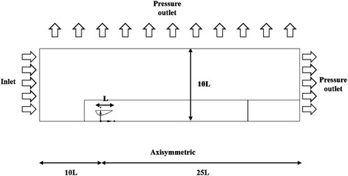
The boundary conditions are related to axisymmetric conditions at the bottom, gauge pressure at outlets, inlet wind speed, turbulence intensity, and no-slip conditions at walls.

2.4. Automation for geometry generation

An automated script was developed using Ansys SpaceClaim to streamline the process of generating geometry and reduce the time required for manual geometry creation. This script takes input parameters, which are variables of study, and automatically generates the corresponding geometry by transforming these input parameters into a Bezier Curve. A flowchart describing the algorithm used to achieve this geometry generation automation is shown in Figure 4.

Figure 4. Algorithm flowchart for Bezier Curve's control points determination.

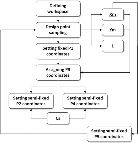
The script was written in IronPython, a programming language integrated into Ansys SpaceClaim. Following the application of the script, a 2D geometry is generated for parametric analysis and CFD simulations. This automated approach saves time and ensures consistency in the geometry generation process, enhancing accuracy. Furthermore, this automated procedure, aimed at streamlining the design process, underscores the significance of utilising software tools and programming languages to address the complexities of aerodynamic design.

2.5. Computational mesh

Mesh optimisation is critical to enhance computational efficiency during CFD simulations as it directly affects computational costs. For this purpose, an unstructured mesh has been chosen due to its flexibility in adapting to complex blade geometries and streamlining mesh generation. This method divides the computational domain into minor irregular elements with triangular shapes instead of regular grids.

Figure 5 displays three Bodies of Influence, which divide the computational domain. A growth factor is implemented to ensure mesh refinement on these three bodies, enabling local refinement in areas of interest to enhance accuracy as required without unreasonably increasing computational cost throughout the domain. This technique effectively balances computational efficiency and solution accuracy, making it appropriate for this application.

Figure 5. Computational meshing and inflation.

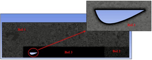
The size of the first Body of Influence on the EC’s walls is determined to satisfy the y+ = 1 criterion, with an inflation of 25 layers and a growth rate of 1.2, as depicted in Figure 5. Optimising the mesh size and structure reduces computation time while maintaining a sufficiently high level of accuracy in CFD simulations.

In addition, when evaluating mesh quality, it is crucial to consider two main factors: asymmetry and orthogonal quality. These quality metrics indicate the mesh’s reliability and ability to represent the computational domain.

2.6. Grid convergence analysis

To perform a sensitivity analysis of the results concerning mesh refinement, three types of mesh are selected as case studies: refined, medium, and coarse. Celik’s Grid Convergence Index (GCI) approach is employed to quantify discretization errors (Celik et al. 2008). The GCI method allows for assessing the impact of mesh refinement on the accuracy of results, providing an indicator of the convergence of the solution.

The usual mesh size ℎ is determined, along with three sets of grids: fine ($N1$), medium ($N2$), and coarse ($N3$). All three output variables are then calculated based on simulations run for each grid ($\varphi 1,\varphi 2,\varphi 3$). Based on empirical knowledge and previous studies (Trentin et al. 2022), the grid refinement factor ($r$) must be greater than 1.3.

Afterward, the mesh quality is evaluated by considering its orthogonal quality and skewness. Meshing details obtained from the sensitivity analysis and discretization error are provided in Table 2.

Table 2. Grid Convergence Index specifics.

GCI parameters	Values
$N1$	448,494
$N2$	226,665
$N3$	152,699
R21	1.403
R32	1.401
$\varphi 1$	1.703
$\varphi 2$	1.696
$\varphi 3$	1.685
GCI	0.381%

The analytical procedure presented by (Celik et al. 2008) describes the calculation procedure for GCI values, as described in (Calle, Baca, and Gorizales 2022). Numerical uncertainty for medium and fine meshes falls within acceptable limits. Therefore, the medium mesh is selected for the present study to run CFD simulations.

III. Methodology based on the metamodel of optimal prognosis

3.1. Methodology outline

The methodology employed for parameter optimisation is primarily grounded in the Metamodel of Optimal Prognosis, as elucidated in (Calle, Baca, and Gorizales 2022), which has been modified to better cope with the challenges and accuracy required by the present study.

This proposed methodology comprises a systematic sequence of steps following a particular methodological framework outlined below:

• Design of Experiment: This initial phase involves identifying the underlying techniques and the set of variables of interest, along with their corresponding target variable to be optimised.

• Geometry Parameterization: Bezier Curves are employed for the geometry parameterisation (Khalid et al. 2020) of the Eolic Cell’s Internal Aerodynamic Chamber (IAC).

• Sampling Method: Advanced Latin Hypercube Sampling (LHS) is applied to sample several design points across the workspace (Loh 1996).

• CFD Simulations Configuration: This step entails configuring CFD simulations, encompassing meshing, boundary conditions, turbulence models, and relevant parameters.

• Parameter Sensitivity Analysis: A sensitivity analysis is conducted over sampled design points by analyzing results from CFD simulations.

• Metamodel of Optimal Prognosis (MOP): The MOP is applied to generate corresponding response surfaces for both the workspace and the zone of interest. These response surfaces are subject to a coefficient of prognosis threshold (Most and Will 2008) set at a minimum of 99%.

• Gradient-based Optimisation Process: Optimisation is achieved by applying three gradient-based optimisation models executed on the response surface within the designated zone of interest.

• Consistency Verification: Individual CFD simulations are run at an optimal specific point to secure consistency.

• Optimal Geometry: Optimal geometry is generated for each inlet wind speed.

Figure 6 provides a comprehensive flowchart illustrating the sequence and techniques encompassed in this methodology. It offers a detailed breakdown of the steps involved in creating response surfaces for both the workspace and the zone of interest, distinctly and sequentially. Furthermore, Figure 6 introduces additional feedback points during the CFD simulation configuration and the geometry parameterisation steps since inaccuracies may manifest at either stage.

Figure 6. Flowchart of the proposed two-stage methodology for the optimisation process.

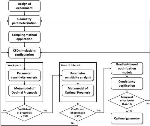
It is imperative to emphasise that the parametric sensitivity analysis, the MOP technique, and the subsequent creation of response surfaces entail two inherent stages for obtaining and refining results, as depicted in Figure 6. The first stage entails running a process across multiple design points spanning the entire workspace. In contrast, the second stage repeats the same process over several design points but within a more confined workspace, referred to as the ‘zone of interest.’ This zone corresponds to the workspace area where the target variable exhibits the highest output values. Consequently, based on this bounded zone of interest, the final response surface attains a higher level of accuracy, which significantly benefits the subsequent application of gradient-based optimisation models.

Additionally, to ensure the precision of all response surfaces, the methodology incorporates thresholds based on a minimum coefficient of prognosis.

3.2. Design of experiment

3.2.1. Variables of interest for geometry optimisation

The magnitude of the augmentation effect relies primarily on the geometric dimensions and aerodynamics of the EC (Calle, Baca, and Gorizales 2022). Consequently, the magnification effect can be expressed as a function dependent on the following key variables, as depicted in Figure 7: throat radius (Ym), throat distance from inlet opening (Xm), chord length (L), inlet opening diameter, outlet opening diameter, and the characteristics of the internal aerodynamic chamber (IAC).

Figure 7. The EC's geometric dimensions represent independent variables.

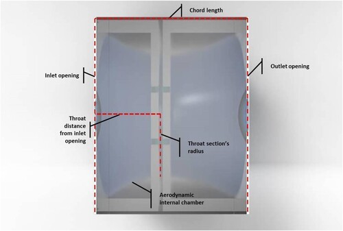
Moreover, since the throat diameter and inlet opening diameters are interrelated, outcomes from those variables over the augmentation effect become interdependent. The augmentation effect is caused, in part, by the differential pressure created around and within the EC, which is driven and intensified by different proportions of the throat diameter over the openings’ diameter, holding other factors constant. Thus, the reason behind this interdependence is explained by the ratio of throat diameter over inlet opening diameter (RTO), given that the inlet and outlet openings have the same diameter.

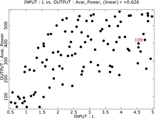
Assuming constant inlet and outlet opening diameters, Figure 8 depicts 2D Anthill representations where the correlation between the throat diameter and available power (P) is illustrated.

Figure 8. 2D Anthill represents the existing correlation between throat radius (Ym) and respective available power (Avai_Power).

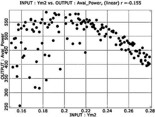
Thus, the influence of both throat diameter and opening diameter on the wind speed augmentation effect remains equal, regardless of their magnitudes, as long as RTO remains constant. In other words, everything else being equal, a random plot of both variables could yield redundant information, as RTO would consistently replicate with different underlying dimensions. Consequently, to model these two variables effectively, one must be held constant while allowing the other to vary freely. In this study, the opening diameters are kept constant at 0.8 meters, while Ym becomes the variable of interest.

In contrast to the study (Calle, Baca, and Gorizales 2022), which focused solely on two geometric input variables, Ym and Xm, it disregarded the impact of the EC’s chord length on the average wind velocity (AWV). However, preliminary exploratory simulations have shown a significant coefficient of importance on the augmentation effect, where L significantly influences the final output. Figure 9 illustrates the correlation between L and P for a given entry wind speed.

Figure 9. 2D Anthill represents the existing correlation between chord length (L) and respective available power (Avai_Power).

The main objective of this study is to maximise wind power density through the augmentation effect. To achieve this, the research focuses on an expanded set of variables, referred hereafter as input variables for optimisation: Ym, Xm, and L.

3.2.2. Target variable for maximisation

The decision to optimise the EC parameters to maximise the power density was based on the research conducted by Bagheri-Sadeghi et al. (Bagheri-Sadeghi, Helenbrook, and Visser 2021), as mentioned in the introductory section. In that study, the optimisation of the total power per unit area in wind turbines was addressed using incompressible RANS equations with the SST k − ω turbulence model (Menter 1994). This previous approach justifies the selection of available power as the primary variable to be maximised in the present study.

In the study (Calle, Baca, and Gorizales 2022), the experimental design aimed to enhance the wind speed augmentation effect by maximising the AWV in the throat section of the EC. However, the same study (Calle, Baca, and Gorizales 2022) concluded that this approach had limitations due to the nonlinearity of the mean wind velocity profiles as the target variable.

By performing CFD simulations following (Calle, Baca, and Gorizales 2022), it was determined that optimising the AWV was unsuitable due to inconsistent results revealed in a sensitivity analysis. Detailed results are presented using the isotropic kriging approximation method (Cressie 1990) in Figure 10.

Figure 10. Isotropic Kriging approximation of average velocity as a function of Xm and Ym.

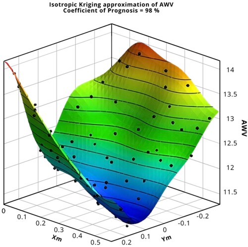
In this figure, it is observed that the AWV is maximised as Ym increases, which, according to the Bezier curve equations, corresponds to a larger diameter. However, it is also evident that the response surface exhibits a valley around Ym = 0.1. Furthermore, it is observed that as Ym decreases in the negative zone, AWV is maximised, indicating a smaller diameter for the turbine, according to the Bezier curve. These results highlight the lack of coherent correlation for effectively implementing the wind turbine rotor in the Eolic Cell, thereby underscoring the inconsistencies associated with maximising AWV to achieve greater power in the wind turbine.

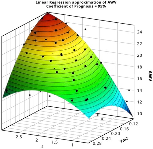
For the present study, initial exploratory simulations were conducted to assess the performance of AWV under a new set of input variables (Ym, Xm, and L). Figure 11 illustrates a response surface representing AWV resulting from the interaction between Ym and L. According to this surface, reducing Ym increases AWV as L increases. In essence, achieving significant AWV may involve reducing throat diameter, which could lead to an insignificant amount of wind power available for harnessing and, consequently, a negligible augmentation effect. In summary, the study must reconsider the wind velocity augmentation effect, as it may be biased toward smaller throat diameters.

Figure 11. Response surface depicts AWV due to the interaction between throat radius (Ym) and chord length (L). The surface response generated has a coefficient of prognosis of 95%.

In light of the identified limitations and the need to obtain more consistent and effective results in this study, the optimisation approach has been shifted towards maximising power density rather than AWV. This decision is congruent with the understanding that available power is the accurate measure of wind energy efficiency in the context of convergent-divergent ducted turbines, thus ensuring a more fundamental study with more consistent results.

Therefore, in order to obtain consistent results compared to the previous AWV, P at the throat section was proposed to replace AWV as the target variable for optimisation. It is essential to establish that available power must be understood as a direct expression of the following equation (6): (6) $P={\displaystyle \frac{1}{2}.\rho .S.{\upsilon }^3}$(6) Where available power (P) is determined by multiplying 0.5 with air density (ρ), the surface of reference (S), and wind speed cubed (${\upsilon }^3$). Additionally, the surface of reference (S) corresponds to the throat section surface area, and the wind speed ($\upsilon$) represents the AWV at the throat section.

The following reasons support the selection of available power (P) as the target variable for the present study: (i) the equation for P incorporates the effect of the former target variable (AWV); moreover, (ii) P considers implicitly in its mathematical expression the Ym, which has a relevant impact on the power augmentation effect due to being the underlying variable responsible for the size of the surface of reference (S).

Furthermore, the power augmentation effect at the throat section can be directly calculated from available power by dividing the cubed AWV at the throat section by the cubed wind speed at ambient conditions, as specified in equation (7): (7) $\mathrm{Power}\mathrm{augmentation}\mathrm{effect}={\displaystyle \frac{P_1}{P_0}={\displaystyle \frac{\left[{\displaystyle \frac{1}{2}.\rho .S.{\left(v_1\right)}^3}\right]}{\left[{\displaystyle \frac{1}{2}.\rho .S.{\left(v_0\right)}^3}\right]}={\displaystyle \frac{{\left(v_1\right)}^3}{{\left(v_0\right)}^3}}}}$(7) Where, with all other factors held constant, $v_1$ represents the AWV at the throat section, and $v_0$ denotes the inlet wind speed.

Hence, P emerges as an output variable that better reflects the study’s primary objective, which is to enhance the power augmentation effect while acknowledging the significance of AWV.

3.2.3. The significance of the weighted average wind velocity

The nonlinearity of the wind velocity profiles within the EC’s throat section introduces challenges to the effectiveness of AWV as a fundamental variable for the power augmentation effect.

Figure 12 depicts nonlinear wind velocity profiles obtained from CFD simulations at various wind speeds (Calle, Baca, and Gorizales 2022). These profiles illustrate the radial distribution of wind velocity magnitude at each node within the EC’s throat section. Notably, the minimum wind velocity occurs at the center of the throat section (left side), while the maximum is observed at the throat section’s wall (right side). The decrease in wind velocity on the right side can be attributed to its proximity to the throat section’s boundary, adhering to a non-slip condition.

Figure 12. Nonlinear wind velocity profiles (Calle et al. December 2022).

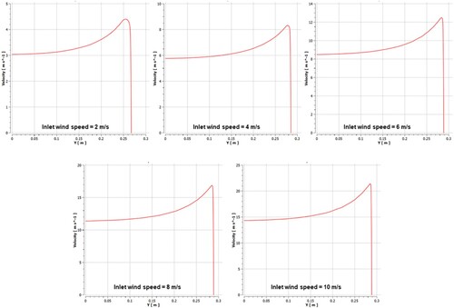
Two significant observations stem from this figure. First, the slope of the nonlinear wind velocity curves varies with wind speed (WS). Second, the overall span length across the throat section differs for each nonlinear wind velocity profile (Calle, Baca, and Gorizales 2022).

In this context, the AWV is inadequate to evaluate the available power (P) since the average wind velocity at the nodes does not consider the variations of the flow volume passing through each node. This inadequacy arises from the oversimplified assumption that the wind velocity profile is linear, disregarding the significance of nonlinear flow volume. Furthermore, segments closer to the throat section’s wall hold greater relevance for power availability than those nearer to the throat section’s center, as wind flow volume increases with throat radius (Ym).

To enhance the precision of power augmentation effect calculations, it becomes imperative to employ a weighted AWV. This approach involves assigning weights to wind velocity at each node based on its corresponding wind flow volume. Consequently, the conventional AWV is replaced by a mass-weighted average wind velocity as the foundational variable for computing P and, subsequently, the power augmentation effect.

3.3. Geometry parameterisation

The IAC of eolic cells plays a crucial role in enhancing the velocity of the wind. The wind passes through the converging section, where its velocity increases due to a decrease in cross-sectional area. As the wind enters the diverging section, the velocity decreases due to an increase in cross-sectional area. This change in velocity creates a pressure difference, which results in a wind velocity increase at the EC’s throat section.

Bezier curves are used to parameterise the dimensions of an eolic cell. These curves are mathematical representations of shapes that are created using control points. They are commonly used in computer graphics and modeling. By adjusting the control points, the shape of the Bezier Curve can be modified to achieve the desired dimensions of the eolic cell, allowing for greater control over the wind flow and corresponding optimisation process.

The Bezier Curves’ geometry parameterisation application is explained in greater depth in Chapter IV (‘Parameter optimization and its corresponding results’).

3.4. Sampling method application

The advanced Latin Hypercube Sampling (LHS) is applied to select design or support points across the workspace and zone of interest, respectively.

The LHS is a statistical method used in various fields, including engineering and scientific research, to explore the parameter space and identify optimal design points efficiently. Advanced LHS is an enhanced version of this method that allows for selecting multiple design points across the workspace to obtain a representative sample of the parameter space while minimising the number of simulations required. This technique is particularly useful in complex systems where the number of input variables is large, and the computational cost is high. Applying advanced LHS can lead to significant time and cost savings in designing and optimising complex systems.

3.5. CFD simulations configuration

Computational Fluid Dynamics (CFD) simulations are a complex process that involves several steps. The first step is meshing, which divides the domain into small, manageable elements. The second step is defining boundary conditions, which specify fluid behaviour at the domain’s boundaries. The third step is selecting the appropriate turbulence model and its parameter values, which are used to calculate the effects of turbulence on fluid flow. These steps are crucial in obtaining accurate results in CFD simulations.

CFD simulations for this study are executed with meshing, boundary conditions, and turbulence models as described in the ‘Computational fluid dynamic configuration’ section.

3.6. Parameter sensitivity analysis

A parametric sensitivity analysis evaluates how changes in inputs to a system affect the output of that system. In this case, sampled design points are being analyzed by conducting CFD simulations to determine how sensitive the results are to changes in the input variables. This analysis helps identify which input variables have the most significant impact on output, allowing for system design optimisation.

3.7. Metamodel of optimal prognosis

Different geometries and parameter variations must be tested in the workspace to improve a design using gradient-based methods. However, conducting these optimisations can be computationally expensive. To overcome this challenge, an MOP can be utilised to obtain gradient-based optimisation results, eliminating the need to run multiple costly CFD simulations for each optimisation model.

After performing a sensitivity analysis, a response surface is created using the MOP application. It is essential to verify the feasibility of this response surface by removing any outliers and evaluating the coefficient of determination, coefficient of importance, and coefficient of prognosis, respectively.

To not compromise the accuracy and efficiency of the optimisation process, it is important to keep in mind that as the number of variables increases, the ability to predict outcomes from parameter response surfaces decreases. Therefore, it is recommended to limit the use of gradient-based optimisation methods to a moderate number of parameters whenever possible.

After applying a sampling method to generate design points across the workspace, MOP uses numerical simulation outcomes to determine an optimal approximation model from which response surfaces are derived (Most and Will 2010).

3.7.1. Coefficient of determination

The coefficient of determination (COD) is a statistical measure commonly used to evaluate the fitness of a polynomial regression model. It is a value that ranges between 0 and 1, where a value of 1 indicates a perfect fit between the model and the data, and a value of 0 implies the opposite. In other words, it measures the extent to which the model can explain the variability in the data. It represents the proportion of the variance in the dependent variable that is predictable from the independent variable(s) (Montgomery and Runger 2010).

COD is calculated by comparing the total sum of squares ($S{S}_T$) with the residual sum of squares ($S{S}_R$), as in equation (8). $S{S}_T$ is the sum of the squared differences between the actual dependent variable values and the mean of the dependent variable, whereas $S{S}_R$ is the sum of the squared differences between the actual dependent variable values and the predicted values from the regression model. (8) $R^2={\displaystyle \frac{S{S}_R}{S{S}_T}=1-{\displaystyle \frac{S{S}_E}{S{S}_T},0\ll R^2\ll 1}}$(8) Equation (8) describes variance components where the overall variability using the total sum of squares ($S{S}_T$) explains the total variation in the output being examined. However, since not all variability can be explained by the approximation model, the regression sum of squares ($S{S}_R$) is calculated, which measures the amount of variation that can be attributed to the regression model. The remaining variability in the dataset, which the regression cannot explain, is captured by the residual sum of squares ($S{S}_E$). The underlying factors contributing to the variation in the analyzed approximation model can be better understood by breaking down the total variation into its components.

When the COD is high, the independent and dependent variables in the model have a strong relationship. Conversely, when the COD value is low, the model does not accurately represent the input data and should be improved (Montgomery and Runger 2010).

3.7.2. Coefficient of importance

The coefficient of importance (COI) is a statistical measure derived from the COD to estimate the significance of input variables with respect to the output variable. The COD implicitly considers the degree of correlation between the input and output variables. The COI can be used to identify which input variables have a greater impact on the output variable and, therefore, should be given more attention during analysis. COI provides insights into the relationship between input and output variables (Most and Will 2008). By focusing on influential input variables, informed decisions can be made regarding the optimisation process. (9) $\mathrm{CoI}\left(X_i,Y\right)=R_{Y,X}^2-R_{Y,X\sim i}^2$(9) According to equation (9), to determine the COI for a single variable (X_i) in predicting an output (Y), a polynomial model can be used. The COI is based on two factors: the COD of the entire model, which includes all variables ($R_{Y,X}^2$), and the COD of a reduced model, excluding all interaction terms for the variable of interest ($R_{Y,X\sim i}^2$).

An input variable has low importance when its specific COI is close to one, indicating that collecting more data on that variable may be necessary to improve accuracy or eliminate such a variable without significantly affecting the model’s accuracy. On the other hand, an input variable is considered highly important when its specific COI is close to zero, pointing out that it may be possible to reduce the amount of data collected on that variable without significantly impacting accuracy.

3.7.3. Coefficient of prognosis

Exploring potential metamodels involves evaluating the quality of the prognosis that each can provide. This evaluation uses an objective measure known as the Coefficient of Prognosis (COP). The COP is a quantitative measure that offers a way to compare the effectiveness of different metamodels. (10) $\mathrm{COP}=1-{\displaystyle \frac{S{S}_E^{\mathrm{Prediction}}}{S{S}_T}}$(10) According to Equation (10), COP is calculated by comparing the predicted outcomes of the metamodel ($S{S}_E^{\mathrm{Prediction}}$) with the actual outcomes ($S{S}_T$). If the predicted outcomes closely match the actual outcomes, then the COP will be close to one, indicating a good prognosis quality. On the other hand, if the predicted outcomes do not match the actual outcomes, then the COP will be close to zero, indicating a poor prognosis outcome.

By analyzing the COP for each metamodel, it can be determined which metamodel provides the highest quality of prognosis. It means the metamodel with the highest COP will most effectively ensure accurate and reliable prognoses.

3.7.4. Kriging approximation

Kriging approximation is a geostatistical method used for spatial prediction. It is a well-established technique that allows interpolation and estimation of values at unsampled locations based on the values of surrounding sample points, providing accurate and reliable estimates. The method minimises the mean error of the weighted sum of sampling values, where the spatial correlation between the sample points determines the weights (Cressie 1990). This approach ensures that the predicted values are unbiased and optimal in terms of variance, making it a reliable method for spatial prediction.

Kriging employs a statistical model to calculate the spatial correlation between the sample points, which is used to estimate the values at unsampled locations (Cressie 1990). The model assumes that the spatial correlation between the sample points is stationary, meaning it does not change with distance or location.

3.8. Gradient-based optimisation process

For the optimisation process, three different gradient-based optimisation models are utilised. These models are designed to fine-tune the system’s performance by analyzing respective response surfaces to improve performance. The response surface, the relationship between the system’s inputs and outputs, is assessed within a specific zone of interest to gain insights into its inherent shape. The optimisation process involves analyzing response surface gradients to maximise output. Thus, optimal results can be achieved while reliably improving the system’s performance.

Specific gradient-based models utilised for the present study are described in the subsection ‘Results and specifics of the optimization process.’

3.9. Consistency verification

To ensure consistency and MOP predictability capacity, a single CFD simulation is run at the optimal point obtained through gradient-based optimisation models. Subsequently, the result is compared to a threshold of margin error that must remain below 1%. The optimisation process must be repeated if the margin error exceeds this threshold.

3.10. Optimal geometry generation

Upon completing the consistency verification process, an optimised geometry is generated based on the optimal design point. This optimised geometry is, thus, the result of a thorough analysis and ensures that the optimal design meets the desired requirements.

IV. Parameter optimisation and its corresponding results

4.1. Geometry parameterisation through Bezier Curves

To transform the geometric parameters of the EC into computable data suitable for CFD simulations, fourth-degree Bezier Curves (4dBZC) were employed. These curves were chosen based on their effectiveness in spanning the entire workspace, enabling the exploration of a broad range of computable geometries. The selection of these curves incurred a higher computational cost due to the necessity of adequately representing the required convex geometries for this study (Calle, Baca, and Gorizales 2022). In a nutshell, 4dBZC offers a more accurate numerical representation of the EC’s geometric parameters.

Figure 13 illustrates a 4dBZC representing the convex geometry of an EC’s IAC.

Figure 13. Fourth-degree Bezier Curve and respective control points.

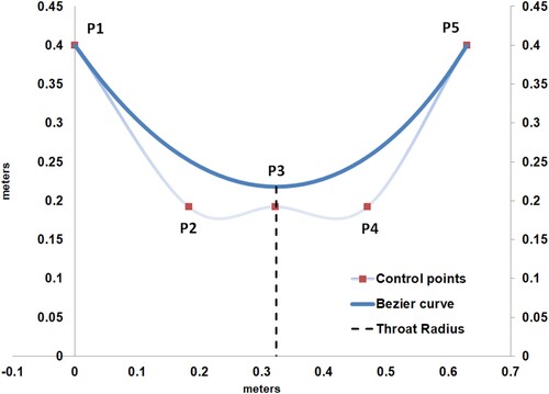
The geometric parameters of the EC (Ym, Xm, and L) are linked to its control points, which are adjusted along the axes of the workspace. The x-axis corresponds to the material dimensions of the EC, representing L, while Ym shares the same y-axis. Xm is associated with the x-axis since it extends along the chord length, eliminating the need for an additional dimension.

Consequently, the workspace is defined within the scale of [0–5.0] for the x-axis and [0.1–0.4] for the y-axis. The input variables are scaled accordingly: [0–1.0] for Xm, [0.1–0.35] for Ym, and [0.5–5.0] for L. These ranges have been determined based on preliminary CFD simulations, approximating the region where optimal design points are expected.

In practical terms, these scales mean that the x-axis ranges from 0 to 5.0 meters, representing both L and Xm. Specifically, L spans from 0.5 to 5.0 meters, and Xm covers 0–1.0 meters. The y-axis, representing Ym, ranges from 0.1 to 0.35 meters. These ranges have been chosen based on the findings of earlier CFD simulations to exclude irrelevant results in relation to the power augmentation effect.

To ensure a valid optimisation process, avoiding redundant or non-convex geometries is crucial. Thus, the unconstrained sampling of design points (support points) is bounded to keep geometries within a reasonable range. An algorithm is applied to limit the degrees of freedom of the 4dBZC according to (Calle, Baca, and Gorizales 2022), which has been modified to include the chord length as a new input variable, where control point P5 has been given specific degrees of freedom to accommodate this change. The following steps detail how the algorithm is adapted for the new set of input variables:

• Step 1: Defining the workspace.

Workspace coordinates span from [0–5.0] for the x-axis to [0.1–0.4] for the y-axis.

• Step 2: Design points sampling.

Advanced LHS generates random design points for input variables within their specified working ranges.

• Step 3: Make control point P1 fix.

P1 remains fixed at coordinates [0; 0.399], representing the entry point of the EC.

• Step 4: Make control point P3 variable.

Assign the design point to control point P3, where P3 receives the corresponding Bernstein polynomial values (Phillips and Phillips 2003) derived from Xm and Ym.

• Step 5: Make control points P2 and P4 a function of P3.

Control points P2 and P4 are semi-fixed and become functions of control point P3 by assigning a strain coefficient (Cs). P3 remains an input variable, while the strain coefficient remains constant at 1.5. Further details on the function of P2 and P4 can be found in Table 3.

• Step 6: Make control point P4 a function of L.

Table 3. Specifics of the algorithm to limit the degrees of freedom for sampling each design point.

Control point	Type	x-axis coordinate	y-axis coordinate
P1	Fixed	0	0.399
P2	Semi-fixed	$f\left(P3,\mathrm{Cs}\right)=(\mathrm{Xm}{)}^{\mathrm{Cs}};$ where Cs $=1.5$	Equal to (Ym) from P3
P3	Mobile	Xm = [0–1.0] Random sampling	Ym = [0.1–0.35] Random sampling
P4	Semi-fixed	$f\left(P3,\mathrm{Cs}\right)=(\mathrm{Xm}{)}^{{\displaystyle \frac{1}{\mathrm{Cs}}}}$; $\mathrm{where}\mathrm{Cs}=1.5$	Equal to (Ym) from P3
P5	Semi-fixed	$\mathrm{Equal}\mathrm{to}\left(L\right)$; $\mathrm{where}L>1.5\left(\mathrm{Xm}\right)$	0.399

Semi-fixed control point P5 is adjusted as a function of L. A constraint is applied, requiring that L must be a minimum of 1.5 times equivalent to Xm. More details on the function of P5 are available in Table 3.

• Step 7: Repeating steps.

Finally, repeat steps 2–6 for each sampled design point.

Where P1, P2, P3, P4, and P5 correspond to control points, according to Figure 13. On the other hand, the strain coefficient (Cs) relates to a factor affecting the gradient of the geometry’s convex shape, which must be greater than 1. A small strain coefficient delivers a more linear and acute geometry, whereas a significant strain coefficient conveys a smoother and more curved geometry. It is important to note that strain coefficients lower than 1.0 would generate non-plausible geometries. For the present study, the strain coefficient applied to the algorithm was discretely selected for convenience and simplification, assuming that such a variable has a marginal impact on the power augmentation effect. Further studies are necessary to confirm this assumption.

Figure 4 provides a general flowchart of the algorithm, serving as the foundation for the automated geometry generation (refer to Section 2.4).

Table 3 summarises the specific configuration of the algorithm applied to each control point for geometry parameterisation.

Following the application of the algorithm, the degrees of freedom for the 4dBZC are limited from five random control points to just one random control point. It means that, by following the algorithm sequence, one control point (P1) remains fixed, while the other three control points (P2, P4, P5) become functions of a single input variable (P3) representing the sampled design point.

Furthermore, since control points’ coordinates differ from physical coordinates, they must be converted to accurately represent the IAC’s geometry. To calculate the actual Xm and Ym, a fourth-degree Bernstein polynomial equation is applied. To derive the physical coordinates, ‘t’ must be set to 0.5, ensuring that the Bezier Curve’s first derivative equals 0, pinpointing the throat section’s location. In essence, equation (11(11) $P_0(1-t{)}^4+P_{1}4t(1-t{)}^3+P_{2}6t^2(1-t{)}^2+P_{3}4t^3(1-t)+P_4{t}^4$(11) ) enables the determination of the physical coordinates for the throat section within the workspace, with the x-coordinate representing Xm and the y-coordinate representing Ym (Calle, Baca, and Gorizales 2022). (11) $P_0(1-t{)}^4+P_{1}4t(1-t{)}^3+P_{2}6t^2(1-t{)}^2+P_{3}4t^3(1-t)+P_4{t}^4$(11) Where P_i corresponds to the control points of the fourth-degree Bezier Curve.

4.2. Parametric sensitivity analysis

Design points for the parametric analysis are determined by specific input parameters, namely, the throat distance from the inlet opening (Xm), the throat section’s radius (Ym), the chord length (L), and the inlet wind speed (WS). Regarding WS, the input parameters are discretized into the following values: 2, 4, 6, 8, and 10 m/s. These WS values have been intentionally chosen to represent wind conditions suitable for distributed generation. The sampled design points, often referred to as support points, serve as the foundation for generating the response surface, as detailed in the following section.

4.3. Response surfaces generation and assessment

Two sets of response surfaces are generated for each WS: one covering the entire workspace and another focusing on the zone of interest. A total of ten response surfaces are required to perform individual parametric sensitivity analyses using Ansys and Optislang. Following the methodology outlined in the previous section, design points are generated using advanced LHS, and subsequently, a CFD simulation is executed for each sampled point to create corresponding response surfaces, gathering essential data for each WS.

It is important to mention that parametric analysis is conducted through OptiSlang. In contrast, CFD simulations are run using Ansys Fluent, Ansys Meshing, and Ansys Spaceclaim, all operating systematically within Ansys Workbench 2022-R2.

Table 4 summarises metrics related to the response surfaces covering the entire workspace for a given WS, including the number of design points and the power augmentation effect.

Table 4. Metrics summary of the response surfaces on the entire workspace.

Inlet wind speed (m/s)	Number of design points	Number of failed points	Coefficient of determination (CoD)	Coefficient of prognosis (CoP)	Highest mass-weighted wind velocity (m/s)	Wind velocity augmentation effect (m/s)	Optimus radius (m)	Surface of reference (m2)	Highest available power at throat (W)	Power augmentation effect (times)
2	131	26	0.997851	0.988032	5.2369	2.6184	0.2041	0.1309	11.5114	17.9523
4	89	0	0.996925	0.987320	9.1803	2.2951	0.2260	0.1604	76.0184	12.0888
6	90	0	0.995804	0.987351	13.6310	2.2718	0.2238	0.1573	244.0538	11.7254
8	100	0	0.997530	0.988372	19.3905	2.4238	0.2030	0.1295	578.1161	14.2396
10	95	13	0.999328	0.989588	22.3109	2.2311	0.2282	0.1635	1112.4257	11.1058

Table 4 shows that all response surfaces exceed the methodologically assigned threshold of 99%. It is important to emphasise that these performance metrics represent the highest values among the sampled design points, not the final optimal values, which will be detailed in subsequent sections.

Figure 14 presents 3D response surfaces, each generated based on several design points spanning the workspace. These design points represent specific physical dimensions and available power magnitudes resulting from CFD simulations. The axes on the response surface denote Xm (throat distance from the inlet opening), Ym (throat section’s radius), L (chord length), and Avai_Power (augmented available power at the throat section).

Figure 14. 3D response surfaces for the entire workspace. Renderings are organised in rows and columns, where each row relates to an individual WS over which all renderings correspond to the same response surface but are presented with different axes. Conversely, each column corresponds to a group of response surfaces with the same axes but different WS.

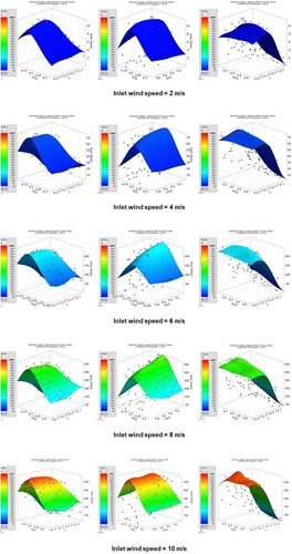
Complementarily, Appendix A displays 2D response surfaces from a top-view perspective, akin to Figure 14, representing the entire workspace where red areas on these surfaces highlight zones of interest with the highest augmented available power.

Results show that the highest augmented available power is found in a concrete area of the workspace, henceforth the zone of interest. Since the remaining workspace does not produce any appreciable gain of P apart from the zone of interest, the additional computational cost is redirected to intensive CFD simulations over the zone of interest to refine the COP and increase accuracy.

The workspace is thus reduced and confined to the zone of interest, where additional design points are sampled, and a larger number of CFD simulations are performed. Notably, according to Appendix A, the zones of interest will vary for each WS depending on the size of the red areas obtained from response surfaces covering the entire workspace.

Table 5 summarises metrics related to response surfaces covering the zone of interest for a given WS. The metrics in this table are the same as those in Table 4.

Table 5. Metrics summary of the zones of interest.

Inlet wind speed (m/s)	Number of design points	Number of failed points	Coefficient of determination (CoD)	Coefficient of prognosis (CoP)	Highest mass-weighted wind velocity (m/s)	Wind velocity augmentation effect (m/s)	Optimus radius (m)	Surface of reference (m2)	Highest available power at throat (W)	Power augmentation effect (times)
2	206	26	0.998737	0.996759	5.1624	2.5812	0.2015	0.1275	10.7480	17.1973
4	188	54	0.998762	0.996159	9.5357	2.3839	0.2157	0.1462	77.6196	13.5483
6	106	0	0.998091	0.995462	13.4932	2.2489	0.2263	0.1609	242.0349	11.3735
8	184	44	0.999248	0.997254	19.0262	2.3783	0.2101	0.1387	585.1839	13.4520
10	162	21	0.999393	0.995088	22.4019	2.2402	0.2323	0.1695	1167.5018	11.2423

Figure 15 showcases response surfaces generated for the zone of interest, emphasising areas with the highest augmented available power for this specific zone of interest.

Figure 15. 3D response surfaces for the zone of interest. Renderings are organised in rows and columns, where each row relates to an individual WS over which all renderings correspond to the same response surface but are presented with different axes. Conversely, each column corresponds to a group of response surfaces with the same axes but different WS.

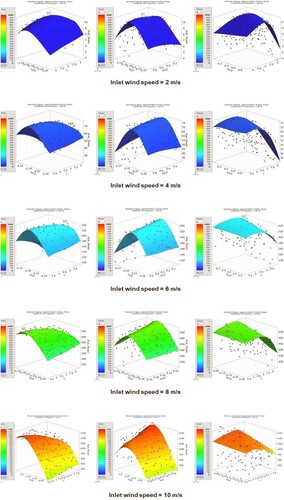
Likewise, Appendix B displays 2D response surfaces for the zone of interest from a top-view perspective. Areas shown in red also represent the most significant augmented available power for the specific zone of interest.

4.4. Results and specifics of the optimisation process

Upon generating response surfaces with a CoP exceeding the 99% threshold, gradient-based optimisation models are employed to approximate sets of design points, from which the final optimal design point is determined. These optimisation models are applied separately for each response surface. Specifically, the utilised gradient-based optimisation models include Nonlinear Programming by Quadratic Langrangian (NLPQL) (Schittkowski 1986), Downhill Simplex Method (Simplex) (Press, Flannery, and Teukolsky 1990; Salcedo and Cândido 2001), and Mix Integer Sequential Quadratic Programming (MISQP) (Exler and Schittkowski 2007).

Subsequently, CFD simulations are performed to compare all potential design point approximations with the predictions made by the optimisation models regarding the maximum available power. Results are considered valid only if they fall within a margin-of-error threshold of 1%. Detailed information about each gradient-based optimisation model is presented in Table 6, Table 7, Table 8, Table 9, and Table 10, along with validation results indicating which models meet the 1% threshold.

Table 6. Specifics about optimisation models’ results for an inlet wind speed of 2 m/s.

Inlet Wind Speed 2 m/s
Gradient-based optimisation model	Optimal design point for [Xm]	Optimal design point for [Ym]	Optimal design point for [L]	weighted average wind velocity (m/s)	Optimised available power (W)	CFD-verified available power (W)	Power augmentation effect (times)	Margin of error	Validation
NLPQL	0.609559	0.179685	2.81136	5.0965	10.7925	10.9010	16.5470	1.0%	Passed
Simplex	0.606554	0.179700	2.81088	5.1003	10.7926	10.9308	16.5839	1.3%	Failed
MISQP	0.855641	0.180167	3.12747	5.0258	10.7960	10.5194	15.8679	2.6%	Failed

Table 7. Specifics about optimisation models’ results for an inlet wind speed of 4 m/s.

Inlet Wind Speed 4 m/s
Gradient-based optimisation model	Optimal design point for [Xm]	Optimal design point for [Ym]	Optimal design point for [L]	Weighted average wind velocity (m/s)	Optimised available power (W)	CFD-verified available power (W)	Power augmentation effect (times)	Margin of error	Validation
NLPQL	1.000000	0.191031	4.61113	9.4999	77.6804	77.7038	13.3961	0.0%	Passed
Simplex	0.333249	0.193700	3.74033	9.3907	76.5661	76.6779	12.9393	0.1%	Passed
MISQP	0.333288	0.193624	3.74458	9.3920	76.5661	76.6649	12.9449	0.1%	Passed

Table 8. Specifics about optimisation models’ results for an inlet wind speed of 6 m/s.

Inlet Wind Speed 6 m/s
Gradient-based optimisation model	Optimal design point for [Xm]	Optimal design point for [Ym]	Optimal design point for [L]	Weighted average wind velocity (m/s)	Optimised available power (W)	CFD-verified available power (W)	Power augmentation effect (times)	Margin of error	Validation
NLPQL	0.002000	0.194070	3.65384	13.8123	244.7140	246.8827	12.1995	0.9%	Passed
Simplex	0.002860	0.194078	3.65478	13.8120	244.7140	246.9554	12.1988	0.9%	Passed
MISQP	0.002000	0.193990	3.65719	13.8152	244.7140	247.1968	12.2073	1.0%	Failed

Table 9. Specifics about optimisation models’ results for an inlet wind speed of 8 m/s.

Inlet Wind Speed 8 m/s
Gradient-based optimisation model	Optimal design point for [Xm]	Optimal design point for [Ym]	Optimal design point for [L]	Weighted average wind velocity (m/s)	Optimised available power (W)	CFD-verified available power (W)	Power augmentation effect (times)	Margin of error	Validation
NLPQL	0.000000	0.194423	3.47060	18.5661	592.0710	595.9927	12.4994	0.7%	Passed
Simplex	0.000001	0.194398	3.47225	18.5396	592.0710	593.3262	12.4459	0.2%	Passed
MISQP	0.000000	0.194358	3.47134	18.5732	592.0710	596.3800	12.5139	0.7%	Passed

Table 10. Specifics about optimisation models’ results for an inlet wind speed of 10 m/s.

Inlet Wind Speed 10 m/s
Gradient-based optimisation model	Optimal design point for [Xm]	Optimal design point for [Ym]	Optimal design point for [L]	Weighted average wind velocity (m/s)	Optimised available power (W)	CFD-verified available power (W)	Power augmentation effect (times)	Margin of error	Validation
NLPQL	0.000000	0.201107	3.19950	22.9117	1176.8700	1180.4363	12.0274	0.3%	Passed
Simplex	0.000010	0.201348	3.21623	22.9156	1176.8400	1183.2537	12.0336	0.5%	Passed
MISQP	0.000000	0.201132	3.19793	22.9247	1176.8700	1182.6654	12.0479	0.5%	Passed

Table 11 displays the optimal design points for each WS, which are determined by comparing valid results to select the design point with the highest augmented available power.

Table 11. Summary of optimal design points per inlet wind speed.

Inlet Wind Speed (m/s)	Optimal design point for [Xm]	Optimal design point for [Ym]	Optimal design point for [L]	Weighted average wind velocity (m/s)	Wind velocity augmentation effect (times)	Optimised Available Power (W)	CFD-verified available power (W)	Power augmentation effect (times)
2	0.6096	0.1797	2.81140	5.0965	2.5482	10.7925	10.9010	16.547000
4	1.0000	0.1910	4.61110	9.4999	2.3750	77.6804	77.7008	13.396100
6	0.00200	0.1941	3.65480	13.8120	2.3020	244.7140	246.9554	12.198800
8	0.0000	0.1944	3.47130	18.5732	2.3217	592.0710	596.3860	12.513900
10	0.0000	0.2011	3.19790	22.9247	2.2925	1176.8700	1182.6654	12.047900

4.5. Optimal design point and optimum geometry equivalent

Optimal design points inherently contain information regarding the optimum geometry. Consequently, the optimum geometry, expressed in meters, can be deduced from the coordinates of the optimal design point. Utilising the Bernstein polynomial equation (11), design point coordinates are converted into physical coordinates. Table 12 summarises the optimal design point coordinates for each WS and their corresponding conversion into physical units (meters).

Table 12. Summary of optimum geometrical profiles per inlet wind speed.

Inlet Wind Speed (m/s)	Optimal design point for [Xm]	Optimal design point for [Ym]	Optimal design point for [L]	Throat distance from inlet opening (m)	Throat section’s diameter (m)	Chord Length (m)
2	0.60956	0.17969	2.81136	0.7030	0.414	2.8110
4	1.00000	0.19103	4.61113	0.1163	0.434	4.6110
6	0.00200	0.19408	3.65478	0.2330	0.439	3.6550
8	0.00000	0.19436	3.47134	0.2170	0.440	3.4710
10	0.00000	0.20113	3.19793	0.2000	0.452	3.1980

4.6. Averaged optimal profile

A proposal for an averaged optimal profile is made based on the observation that optimal geometries tend to exhibit similar physical dimensions. Table 13 outlines the specifics of this proposed averaged optimal profile, including average performance metrics and physical dimensions measured in meters.

Table 13. Specifics of the averaged optimal profile.

Averaged optimal design point for [Xm]	Averaged optimal design point for [Ym]	Averaged optimal design point for [L]	Throat distance from inlet opening (m)	Throat section’s diameter (m)	Chord length (m)	Average wind velocity augmentation effect (times)	Average power augmentation effect (times)
0.33231237	0.1920568	3.549308	0.506	0.436	3.549	2.368	13.341

Table 14 compiles performance data for the averaged optimal profile, considering mass-weighted average wind velocity, wind-velocity augmentation effect, optimised available power, and power augmentation effect at varying WS. The overall performance indicates a power augmentation effect of 12.5 times compared to traditional non-augmented horizontal-axis wind turbines, representing a significant increase in power compared to conventional wind turbines.

Table 14. Performance of the averaged optimal profile given different inlet wind speeds.

Inlet wind speed (m/s)	Throat distance from inlet opening (m)	Throat section’s diameter (m)	Chord length (m)	weighted average wind velocity (m/s)	Wind velocity augmentation effect (times)	Optimised Available Power (W)	Power augmentation effect (times)
2	0.506	0.436	0.3549	4.7864	2.3930	10.0205	13.7070
4	0.506	0.436	0.3549	9.3998	2.3500	75.8959	12.9770
6	0.506	0.436	0.3549	13.7492	2.2920	237.5284	12.0330
8	0.506	0.436	0.3549	18.3078	2.2880	560.7585	11.9850
10	0.506	0.436	0.3549	23.0209	2.3020	1114.8970	12.2000

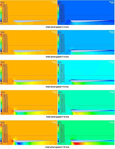
In addition, Figure 16 provides a graphical representation of flow distribution contours for the averaged optimal profile associated with different WS. Because figures are scaled identically, subfigures linked with lower WS are prone to present contours of a similar colour range. In contrast, subfigures coupled with higher WS contours tend to be more distinguishable.

Figure 16. Averaged optimal profile’s flow field distribution contours. Pressure (on the left) and wind velocity (on the right) distribution fields for the averaged optimal profile associated with a specific WS are displayed. The contours in all subfigures are presented under the same scale.

V. Findings

5.1. Optimal profile confinement

A distinct characteristic of the optimal geometrical profiles is their confinement to a narrow workspace region. This confinement is primarily observed because areas with high-power augmentation remain relatively consistent, regardless of changes in wind speed (WS). Figure 17 displays the optimal geometrical profiles categorised by physical dimensions: throat distance from the inlet opening (Xm), throat section diameter (Ym), and chord length (L), all expressed in meters based on data from Table 12.

Figure 17. Chart of optimal profiles’ confinement within the workspace. The optimal profile’s dimensions are organised into groups of physical magnitudes. The vertical axis shows the physical dimensions of each coordinate expressed in meters. Legend in colours shows inlet WS in meters per second (m/s).

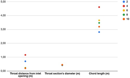
The chart reveals that the confinement of optimal profiles varies among different physical dimensions. For instance, Xm exhibits confinement for WSs above 4 m/s, while dispersion is observed below this threshold. On the other hand, Ym displays confinement to a small region for all WSs, while L shows a low confinement and high dispersion across all wind speeds.

Notably, the dispersion observed in Xm and L at 2 and 4 m/s is associated with relatively flat response surfaces compared to the peaks seen for other response surfaces associated with higher WS (see Figure 15). The flatness of these response surfaces can potentially introduce inaccuracies due to the absence of a clear peak, explaining the apparent misalignment. To enhance accuracy, it is recommended to incorporate a flatness measure into the algorithm in order to increase the number of design points for those cases.

Consequently, the confinement of an optimal profile is primarily applicable to Xm and Ym for WS above 4 m/s. Considering L significantly influences the power augmentation effect and exhibits substantial dispersion across various wind speeds. However, it’s important to note that the dispersion in L falls within the same zone of interest for all WS, indicating that regardless of chord length’s dispersion, the dispersion in the final power augmentation effect would be limited.

Therefore, the zone of interest, defined by physical dimensions, would be restricted to the following ranges: [0.20–0.23] meters for Xm; [0.44–0.45] meters for Ym; and [3.2–3.6] meters for L.

5.2. Power augmentation effect comparison

Table 15 compares the power augmentation effects achieved in the preceding study (Calle, Baca, and Gorizales 2022) and the current study, where the latter outperforms the former by an average factor of 2.69 times.

Table 15. Comparison of results between the preceding paper and the present paper.

Inlet wind speed (m/s)	Preceding paper			Present paper			Improvement
	Average wind velocity (m/s)	Available power (W)	Power augmentation effect (times)	Weighted-average wind velocity (m/s)	Available power (W)	Power augmentation effect (times)	Wind velocity improvement (times)	Power augmentation improvement (times)
2	3.38	6.0	4.81	4.79	17.1	13.71	1.42	2.85
4	6.74	47.6	4.78	9.40	129.4	12.98	1.40	2.72
6	9.89	150.7	4.48	13.75	404.8	12.03	1.39	2.69
8	13.30	366.2	4.59	18.31	955.7	11.98	1.38	2.61
10	16.77	734.5	4.72	23.02	1900.1	12.20	1.37	2.59

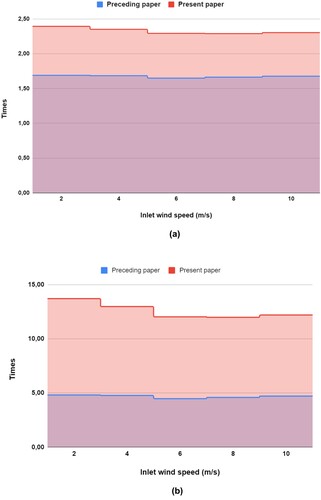
Figure 18 provides a comparison between the average optimal profile proposed in the current study and the average optimal profile from the preceding paper for different wind speeds. The comparison encompasses two key aspects: the wind velocity augmentation effect and the power augmentation effect.

Figure 18. Augmentation effect comparison between the preceding and present papers for the averaged optimal profile. (a) Wind velocity augmentation effect. (b) Power augmentation effect.

5.3. Significance of the chord length on the power augmentation effect

The significant increase in the power augmentation effect observed in the current study can be attributed primarily to including chord length (L) as an input variable for optimisation. Figure 19 illustrates a chart in which chord length (L) exhibits the highest COP coefficient of prognosis among input variables, indicating that L contributes up to 70% to the output response surface for available power (Avai_Power).

Figure 19. Coefficient of prognosis of the input variables.

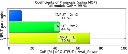
Additionally, Figure 19 reveals that the sum of the coefficients of prognosis for all input variables exceeds 100%. This occurs because the percentages represent the individual contributions of each input variable to the aggregate output variable and interactions between parameters.

Consequently, the results underscore the significance of L in explaining and determining the substantial increase in power (P) and the corresponding power augmentation effect resulting from the optimisation process in the current study.

VI. Conclusions

General conclusions obtained through the discussion and analysis of the data provided by the present study advance insights into performance-related factors and broader aspects of wind power enhancement.

• - The adequacy of the average wind velocity as a target variable is questioned due to its inability to consider the nonlinear wind velocity profile at the throat section, resulting in an inaccurate measurement of wind flow volume and its impact on power augmentation.

• - Available power becomes a more unbiased and robust target variable to account for the power augmentation effect as it considers not only the augmented wind velocity in its calculation but also the volumetric air mass passing through the throat section.

• - To improve the accuracy of the available power calculation, the mass-weighted average wind velocity is applied as the underlying variable instead of the average wind velocity as it accounts for volumetric airflow.

• - Concerning optimisation performance, the power augmentation effect is a more comprehensive measure as it encompasses the wind velocity augmentation effect within its calculation.

Specific conclusions upon the optimisation process performed by the present study are presented below:

• - Optimal geometries are primarily confined to a circumscribed zone of interest within the workspace, specifically regarding the variables related to the throat distance from the inlet opening and the throat section’s diameter. This confinement allows for a single solution to function effectively across a wide range of wind speed conditions.

• - Analysis of the power augmentation effect confirms the substantial potential for power output increase, with available power increasing up to 12.5 times compared to normal non-augmented conditions.

• - Chord length is the most critical input variable, significantly contributing to increased available power and the corresponding power augmentation effect.

• - This study has achieved a 2.7 times improvement in power augmentation effect and available power compared to the previous research.

General implications of the proposed technology for distributed generation:

• - The results do not invalidate previous conclusions regarding the feasibility of employing an averaged optimal profile for various wind resources without significantly compromising the power augmentation effect, making this solution particularly suitable for distributed generation purposes.

• - The combination of an averaged optimal profile and an operating zone of interest enables modularity, facilitating economies of scale for manufacturing purposes.

• - The results further reaffirm the potential of an Eolic Cell to significantly increase available power and potentially serve as an effective wind energy system for distributed generation.

Identified gaps that need to be addressed in future studies are presented below:

• - The study focuses on enhancing the available power but has not examined the effect on the effective power of a wind turbine. Therefore, including a wind turbine rotor in the research project is essential to assess the proposed wind energy system’s significance comprehensively.

• - The present study has omitted the components required to convert wind kinetic energy into electricity generation. In that regard, future studies must cover the intricacies of a power drivetrain and generation systems for a peripherally supported wind turbine proposed by the research project.

Additional research is recommended to fully evaluate the benefits of the EC as a highly efficient wind energy system for distributed generation. See the Recommendations section for more details.

VII. Recommendations

In future studies, a comprehensive understanding of the impact of the IAC’s convex shape on power augmentation should be pursued. This gap can be bridged by investigating the effects of different internal aerodynamic profiles on available power. One way to approach this challenge is by introducing variability in the strain coefficient, a parameter used in geometry formation.

To ensure the findings' validity and prevent potential biases arising from 2D axisymmetric simulations, it is important to replicate the proposed methodology using 3D simulations. This step is essential for confirming conclusions regarding the optimal geometry for the Eolic Cell regarding the power augmentation effect.

Furthermore, for methodological improvement, it is advisable to incorporate a measure to evaluate the flatness at the summit of response surfaces. When a flat surface is detected, it should trigger an increase in the number of design points. This adjustment will enhance the coefficient of prognosis and lead to higher accuracy in the results.

Additionally, to comprehensively assess the potential of an integrated wind energy system, future research should extend its focus beyond optimising the power augmentation effect. This extension should encompass the study of subsystems for wind energy conversion and electricity generation, providing a more holistic understanding of the technology’s capabilities.

Specifically, study subjects to be addressed in future manuscripts should involve, but not be limited to, the performance of a peripherally supported wind turbine embedded within the Eolic Cell, the peripheral power transmission from a wind turbine to a generator system, the conversion of a wind turbine’s kinetic energy into electricity, and the corresponding characterisation of a power curve for the wind energy system and its integrated components.

CRediT author statement

Alfredo R. Calle: Conceptualisation, Methodology, Writing – Original Draft, Formal analysis, Investigation, Visualisation, Project administration. Giusep A. Baca: Methodology, Software, Formal analysis, Investigation. Salome Gonzales: Supervision, Methodology, Resources, Writing – Reviewing and Editing, Funding acquisition. Andrés Diaz: Writing – Reviewing and Editing. Hugo Calderon: Writing – Reviewing and Editing. José López: Writing – Reviewing and Editing.

Acknowledgment

The Universidad Nacional de Ingeniería (UNI) and the Universidad Nacional del Santa (UNS), research parties, also supported the present study.

Disclosure statement

The authors disclose the corresponding financial interest or personal relationship, which may be considered as potential competing interests: Alfredo R. Calle holds a positive patentability report from WIPO #WO2021034203 with a publication date of 25.02.2021.

Data availability statement

The data that support the findings of this study are available from the corresponding author, ARC, upon reasonable request.

Additional information

Funding

This work was supported by ProCiencia under [Grant number PE501078852-2022-PROCIENCIA].

Appendices

Appendix A: 2D top-view response surfaces for the entire workspace

Renderings are organised in rows and columns, where each row relates to an individual WS, in which all figures correspond to the same response surface presented with different axes. Conversely, each column corresponds to a group of response surfaces with the same axes but different WS. The augmented available power is represented in colours, where red depicts the highest values, and blue depicts the lowest.

Appendix B: 2D top-view response surfaces for the zone of interest

Renderings are organised in rows and columns, where each row relates to an individual WS, in which all figures correspond to the same response surface presented with different axes. Conversely, each column corresponds to a group of response surfaces with the same axes but different WS. The augmented available power is represented in colours, where red depicts the highest values, and blue depicts the lowest.

References

- Allaei, D., and Y. Andreopoulos. 2014. “INVELOX: Description of a New Concept in Wind Power and its Performance Evaluation.” Energy 69: 336–344. https://doi.org/10.1016/j.energy.2014.03.021.
- Alpman, Emre. 2018. “Multi-Objective Aerodynamic Optimization of a Microscale Ducted Wind Turbine Using a Genetic Algorithm.” Turkish Journal of Electrical Engineering and Computer Sciences 26 (1): 618–629. https://doi.org/10.3906/elk-1612-307.
- Amer, A., A.H.H. Ali, Y. Elmahgary, and S. Ookawara. 2013. “Effect of Diffuser Configuration on the Flow Field Pattern Inside Wind Concentrator.” In 1st International Renewable and Sustainable Energy Conference, 212–217. IRSEC; 2013. Department of Energy Resources and Environmental Engineering, Egypt-Japan University of Science and Technology, Alexandria, 21934, Egypt.
- Aranake, A.C., and K. Duraisamy. 2017. “Aerodynamic Optimization of Shrouded Wind Turbines.” Wind Energy 20 (5): 877–889. https://doi.org/10.1002/we.2068.
- Aranake Aniket, C., K. Lakshminarayan Vinod, and Duraisamy Karthik. 2013. “Computational Analysis of Shrouded Wind Turbine Configurations.” In 51st AIAA Aerospace Sciences Meeting including the New Horizons Forum and Aerospace Exposition. Stanford, CA, USA: Department of Aeronautics and Astronautics, Stanford University; 2013.
- Aranake Aniket, C., K. Lakshminarayan Vinod, and Duraisamy Karthik. 2015. “Computational Analysis of Shrouded Wind Turbine Configurations Using a 3-Dimensional RANS Solver.” Renewable Energy 75: 818–832. https://doi.org/10.1016/j.renene.2014.10.049.
- Bagheri-Sadeghi, Nojan, Brian T. Helenbrook, and Kenneth D. Visser. 2021. “Maximal Power Per Device Area of a Ducted Turbine.” Wind Energy Science 6 (4): 1031–1041. https://doi.org/10.5194/wes-6-1031-2021.
- Bai, Chi-Jeng, Yang-You Lin, San-Yih Lin, and Wei-Cheng Wang. 2015. “Computational Fluid Dynamics Analysis of the Vertical Axis Wind Turbine Blade with Tubercle Leading Edge.” Journal of Renewable and Sustainable Energy 7 (3): 033124. https://doi.org/10.1063/1.4922192.
- Balijepalli, Ramakrishna, Upendra Rajak, Abhishek Dasore, Anshul Raj, and Prem Kumar Chaurasiya. 2022. “Design and Optimization of NACA 0012, NACA 4412 and NACA 23,012 Aerofoils of Wind Turbine of Solar Updraft Tower Power Plant.” In Technology Innovation in Mechanical Engineering: Select Proceedings of TIME 2021, 9–18. Singapore: Springer Nature Singapore.
- Buehrle, Bridget, Ravi A. Kishore, and Shashank Priya. 2013. “Computational Modeling of Ducted Wind Turbines for Residential Applications.” In ASME 2013 International Mechanical Engineering Congress and Exposition, 6 A, 1–10. IMECE; 2013. CEHMS, Virginia Tech, Blacksburg, VA, United States, 2013. American Society of Mechanical Engineers (ASME).
- Calle, Alfredo R., G.A. Baca, and S. Gorizales. 2022. “Optimization of the Eolic Cell to Improve the Wind Velocity Augmentation Effect Through the Metamodel of Optimal Prognosis.” Energy Conversion and Management: X 16: 100330; December. https://doi.org/10.1016/j.ecmx.2022.100330.
- Celik, Ishmail B., Urmila Ghia, Patrick J. Roache, and Christopher J. Freitas. 2008. “Procedure for Estimation and Reporting of Uncertainty due to Discretization in CFD Applications.” Journal of Fluids Engineering- Transactions of the ASME 130 (7): 078001-1–078001-1.
- Chaurasiya, Prem Kumar, V. Kranthi Kumar, V. Warudkar, and S. Ahmed. 2021. “Evaluation of Wind Energy Potential and Estimation of Wind Turbine Characteristics for two Different Sites.” International Journal of Ambient Energy 42 (12): 1409–1419. https://doi.org/10.1080/01430750.2019.1611634.
- Civalier, G., C. Fridley, J. Li, J. Seabe, A.-X. Stanciu, M. Willey, and R. S. Pant. 2011. “Comparative Analysis of Three Concepts for Aerostat Based Electrical Power Generation System.” In 11th AIAA Aviation Technology, Integration, and Operations (ATIO) Conference, Including the AIAA Balloon Systems Conference and 19th AIAA Lighter-than-Air Technology Conference 2011. Blacksburg, VA, USA: Virginia Polytechnic Institute and State University, Aerospace and Ocean Engineering Department; 2001.
- Coiro, Domenico P., Elia Daniele, and Pierluigi Della Vecchia. 2016. “Diffuser Shape Optimization for GEM, a Tethered System Based on two Horizontal Axis Hydro Turbines.” International Journal of Marine Energy 13: 169–179. https://doi.org/10.1016/j.ijome.2015.08.002.
- Cressie, Noel. 1990. “The Origins of Kriging.” Mathematical Geology 22: 239–252. https://doi.org/10.1007/BF00889887.
- Daniele, E., and D.P. Coiro. 2013. “Optimization of Diffuser Geometry for an Horizontal Axis Shrouded Hydro Turbine.” In: 4th International Conference on Clean Electrical Power: Renewable Energy Resources Impact, 240–247, ICCEP; 2013. Department of Industrial Engineering - Aerospace Section, Universita ` degli Studi di Napoli Federico II, Via Claudio 21, 80125, Napoli, Italy.
- Daniele, E., E. Ferrauto, and D.P. Coiro. 2013. “Horizontal Axis Hydroturbine Shroud Airfoil Optimization.” In 10th International Conference on Advances in Evolutionary and Deterministic Methods for Design, Optimization and Control in Engineering and Sciences, edited by D. Greiner, B. Galvan, G. Winter, N. Gauger, J. Periaux, J. Periaux, and K. Giannakoglou, vol. 36, 241–256. Oldenburg: Springer Netherland, 2015.
- de Vries, O. 1979. “Fluid Dynamic Aspects of Wind Energy Conversion.” AGARDograph (243): 148. ISBN 92-835-1326-6.
- Dighe, V.V., F. Avallone, and G.J.W. van Bussel. 2016. “Computational Study of Diffuser Augmented Wind Turbine Using Actuator Disc Force Method.” International Journal of Computational Methods and Experimental Measurements 4 (4): 522–531. https://doi.org/10.2495/CMEM-V4-N4-522-531.
- Dighe, V.V., F. Avallone, G. Van Bussel, and O. Igra. 2019. “Multi-Element Ducts for Ducted Wind Turbines: A Numerical Study.” Wind Energy Science 4 (3): 439–449. https://doi.org/10.5194/wes-4-439-2019.
- Dighe, V.V., G. de Oliveira, F. Avallone, and G.J.W. van Bussel. 2018. “On the Effects of the Shape of the Duct for Ducted Wind Turbines.” In Wind Energy Symposium. Delft, 2629HS, Netherlands: Wind Energy Research Group, Delft University of Technology. number 210029 2018. American Institute of Aeronautics and Astronautics Inc, AIAA.
- Exler, Oliver, and Klaus Schittkowski. 2007. “A Trust Region SQP Algorithm for Mixed-Integer Nonlinear Programming.” Optimization Letters 1: 269–280. https://doi.org/10.1007/s11590-006-0026-1.
- Fletcher Clive, A.J.J. 1981. “Computational Analysis of Diffuser-Augmented Wind Turbines.” Energy Conversion and Management 21 (3): 175–183. https://doi.org/10.1016/0196-8904(81)90012-1.
- Foote, Tudor, and Ramesh Agarwal. 2012. “Optimization of Power Generation from Shrouded Wind Turbines.” Energy Sustainability: 44816: 1325–1331.
- Foreman, K.M., B.L. Gilbert, and R.A. Oman. 1978. “Diffuser Augmentation of Wind Turbines.” Solar Energy 20 (4): 305–311. https://doi.org/10.1016/0038-092X(78)90122-6.
- Gilbert Barry, L., A. Oman Richard, and M. Foreman Kenneth. 1978. “Fluid Dynamics of Diffuser-Augmented Wind Turbines.” Journal of Energy 2 (6): 368–374. https://doi.org/10.2514/3.47988.
- Hang, Wang Xiao, Chong Wen Tong, Wong Kok Hoe, Wang Chin-Tsan, Saw Lip Huat, Poh Sin Chew, and Lai Sai Hin. 2018. “Preliminary Assessment of Optimized Accessorial Roof Shape for Performance of Wind Turbine Mounted on Eco-Roof System.” International Journal of Precision Engineering and Manufacturing-Green Technology 5: 375–385. https://doi.org/10.1007/s40684-018-0040-7.
- Hu, Ssu-Yuan, and Jung-Ho Cheng. 2008. “Innovatory Designs for Ducted Wind Turbines.” Renewable Energy 33 (7): 1491–1498. https://doi.org/10.1016/j.renene.2007.08.009.
- Huet, Sylvie, and Marie-Luce Taupin. 2017. “Metamodel Construction for Sensitivity Analysis.” ESAIM: Proceedings and Surveys 60: 27–69. https://doi.org/10.1051/proc/201760027.
- Im, Yunhyeok, H. Jo, C. Oh, Y.S. Cho, J. Yoo, H. Lee, M. Lee, and V.K. Yaddanapudi. 2022. “Thermal Model Simplification of Mobile Device with Adaptive Metamodel of Optimal Prognosis (AMOP).” In 2022 21st IEEE Intersociety Conference on Thermal and Thermomechanical Phenomena in Electronic Systems (iTherm). IEEE.
- Jadallah, Abdullateef A., Sahar R. Farag, and Jinan D. Hamdi. 2018. “Performance Enhancement of a Darrius 3-Bladed Wind Turbine Using Convergent-Divergent Ducting System.” Journal of Engineering Science and Technology 13 (7): 1891–1904.
- Jamieson, Peter. 2008. “Generalized Limits for Energy Extraction in a Linear Constant Velocity Flow Field.” Wind Energy 11 (5): 445–457. https://doi.org/10.1002/we.268.
- Jamieson, Peter M. 2009. “Beating Betz: Energy Extraction Limits in a Constrained Flow Field.” Journal of Solar Energy Engineering-Transactions of the ASME 131 (3): 031008–031014.
- Khalid, Waleed, Salma Sherbaz, Adnan Maqsood, and Zamir Hussain. 2020. “Design and Optimization of a Diffuser for a Horizontal Axis Hydrokinetic Turbine Using Computational Fluid Dynamics Based Surrogate Modelling.” Mechanics 26 (2): 161–170. https://doi.org/10.5755/j01.mech.26.2.23511.
- Khamlaj, Tariq Abdulsalam, and Markus Peer Rumpfkeil. 2018. “Analysis and Optimization of Ducted Wind Turbines.” Energy 162: 1234–1252. https://doi.org/10.1016/j.energy.2018.08.106.
- Kumar, Vedant, and Sandeep Saha. 2019. “Theoretical Performance Estimation of Shrouded Twin-Rotor Wind Turbines Using the Actuator Disk Theory.” Renewable Energy 134: 961–969. https://doi.org/10.1016/j.renene.2018.11.077.
- Leloudas, S.N., G.N. Lygidakis, A.I. Eskantar, and I.K. Nikolos. 2020. “A Robust Methodology for the Design Optimization of Diffuser Augmented Wind Turbine Shrouds.” Renewable Energy 150: 722–742. https://doi.org/10.1016/j.renene.2019.12.098.
- Lilley, G.M., and W.J. Rainbird. 1956. “A Preliminary Report on the Design and Performance of a Ducted Windmill.” Technical report.
- Loh, Wei-Liem. 1996. “On Latin Hypercube Sampling.” The Annals of Statistics 24 (5): 2058–2080.
- Mathlouthi, Gino, Simon Kügele, Fatmaalzahraa Elsayed, Ralf Voß, Peter Renze, Michael Kaufeld, and Thomas Grützner. 2023. “Wettability Prediction for 3D-Printed Surfaces Using Reverse Engineering and Computational Fluid Dynamics Simulations.” Industrial & Engineering Chemistry Research 62 (3): 1627–1635. https://doi.org/10.1021/acs.iecr.2c03805.
- Matsushima, Toshio, Shinya Takagi, and Seiichi Muroyama. 2006. “Characteristics of a Highly Efficient Propeller Type Small Wind Turbine with a Diffuser.” Renewable Energy 31 (9): 1343–1354. https://doi.org/10.1016/j.renene.2005.07.008.
- Mehmood, N., Z. Liang, and J. Khan. 2012. “Diffuser Augmented Horizontal Axis Tidal Current Turbines.” Research Journal of Applied Sciences, Engineering and Technology 4 (18): 3522–3532.
- Mehmood, Nasir, Liang Zhang, and Jawad Khan. 2012. “CFD Study of NACA 0018 for Diffuser Design of Tidal Current Turbines.” Research Journal of Applied Sciences, Engineering and Technology 4 (21): 4552–4560.
- Menter, Florian R. 1992. “Improved Two-Equation k-omega Turbulence Models for Aerodynamic Flows.” No. A-92183.
- Menter, Florian R. 1994. “Two-Equation Eddy-Viscosity Turbulence Models for Engineering Applications.” AIAA Journal 32 (8): 1598–1605. https://doi.org/10.2514/3.12149.
- Montgomery, Douglas C., and George C. Runger. 2010. Applied Statistics and Probability for Engineers. Jefferson City: John Wiley & Sons.
- Most, Thomas, and Johannes Will. 2008. “Metamodel of Optimal Prognosis - An Automatic Approach for Variable Reduction and Optimal Metamodel Selection.” Proceedings of Weimarer Optimierungs-und Stochastiktage 5: 20–21.
- Most, Thomas, and Johannes Will. 2010. “Recent Advances in Metamodel of Optimal Prognosis.” Proceedings of the Weimarer Optimierungs-und Stochastiktage 7: 21–22.
- Most, Thomas, and Johannes Will. 2011. “Sensitivity Analysis Using the Metamodel of Optimal Prognosis.” Weimar Optimization and Stochastic Days 8 (0): 1–16.
- Nunes, Matheus M., Antonio C.P. Brasil Junior, and Taygoara F. Oliveira. 2020. “Systematic Review of Diffuser-Augmented Horizontal-Axis Turbines.” Renewable and Sustainable Energy Reviews 133: 110075. https://doi.org/10.1016/j.rser.2020.110075.
- Ohya, Y., and T. Karasudani. 2010. “A Shrouded Wind Turbine Generating High Output Power with Wind-Lens Technology.” Energies 3 (4): 634–649. https://doi.org/10.3390/en3040634.
- Ohya, Yuji, Takashi Karasudani, Akira Sakurai, and Masahiro Inoue. 2006. “Development of a High-Performance Wind Turbine Equipped with a Brimmed Diffuser Shroud.” Transactions of the Japan Society For Aeronautical And Space Sciences 49 (163): 18–24. https://doi.org/10.2322/tjsass.49.18.
- Ohya, Y., T. Uchida, T. Karasudani, M. Hasegawa, and H. Kume. 2012. “Numerical Studies of Flow Around a Wind Turbine Equipped with a Flanged-Diffuser Shroud Using an Actuatordisk Model.” Wind Energy 36 (4): 455–472. https://doi.org/10.1260/0309-524X.36.4.455.
- Oka, Nobuhito, Masato Furukawa, Kazutoyo Yamada, Akihiro Oka, and Yasushi Kurokawa. 2015. “Aerodynamic Performances and Flow Fields of Pareto Optimal Solutions in an Aerodynamic Design of a Wind-Lens Turbine.” In ASME Turbo Expo 2015: Turbine Technical Conference and Exposition, GT 2015, vol. 9. Fukuoka, Japan: Department of Mechanical Engineering, Kyushu University. [American Society of Mechanical Engineers (ASME).
- Oman, R.A., K.M. Foreman, and B.L. Gilbert. 1977. “Investigation of Diffuser-Augmented Wind Turbines. Part II.” Technical report.
- Phillips, George M., and George M. Phillips. 2003. “Bernstein Polynomials.” Interpolation and Approximation by Polynomials, 247–290. https://doi.org/10.1007/0-387-21682-0_7.
- Press, William H., Brian P. Flannery, and S.A. Teukolsky. 1990. “Vetterling, Numerical Recipes: The Art of Scientific Computing”.
- Rahmatian, Mohammad Ali, Amin Nazarian Shahrbabaki, and Seyed Peyman Moeini. 2023. “Single-Objective Optimization Design of Convergent-Divergent Ducts of Ducted Wind Turbine Using RSM and GA, to Increase Power Coefficient of a Small-Scale Horizontal Axis Wind Turbine.” Energy 269: 126822. https://doi.org/10.1016/j.energy.2023.126822.
- Rezaeiha, Abdolrahim, Hamid Montazeri, and Bert Blocken. 2018. “Characterization of Aerodynamic Performance of Vertical Axis Wind Turbines: Impact of Operational Parameters.” Energy Conversion and Management 169: 45–77. https://doi.org/10.1016/j.enconman.2018.05.042.
- Salcedo, R.L.R., and M.G. Cândido. 2001. “Global Optimization of Reverse-Flow Gas Cyclones: Application to Small-Scale Cyclone Design.” Separation Science and Technology 36 (12): 2707–2731. https://doi.org/10.1081/SS-100107221.
- Salem, Hayder, Adel Mohammedredha, and Abdullah Alawadhi. 2023. “High Power Output Augmented Vertical Axis Wind Turbine.” Fluids 8 (2): 70. https://doi.org/10.3390/fluids8020070.
- Santoli, L., A. Albo, D. Astiaso Garcia, D. Bruschi, and F. Cumo. 2014. “A Preliminary Energy and Environmental Assessment of a Micro Wind Turbine Prototype in Natural Protected Areas.” Sustainable Energy Technologies and Assessments 8: 42–56.
- Schittkowski, Klaus. 1986. “NLPQL: A Fortran Subroutine Solving Constrained Nonlinear Programming Problems.” Annals of Operations Research 5: 485–500. https://doi.org/10.1007/BF02739235.
- Shi, W., D. Wang, M. Atlar, B. Guo, and K.-C. Seo. 2015. “Optimal Design of a Thin-Wall Diffuser for Performance Improvement of a Tidal Energy System for an AUV.” Ocean Engineering 108: 1–9. https://doi.org/10.1016/j.oceaneng.2015.07.064.
- Sorribes-Palmer, F., A.S. Andres, A. Figueroa, L. Donisi, S. Franchini, and M. Ogueta. 2017. “Aerodynamic Design of a Wind Turbine Diffuser with OpenFOAM.” In 7th European and African Conference on Wind Engineering. EACWE; 2017. Instituto de Microgravedad Ignacio Da Riva, Universidad Polit´ecnica de Madrid (IDR/UPM), Spain. International Association for Wind Engineering (IAWE).
- Trentin, Pedro Francisco Silva, Pedro Henrique Barsanaor de Barros Martinez, Gabriel Bertacco dos Santos, Elóy Esteves Gasparin, and Leandro Oliveira Salviano. February 2022. “Screening Analysis and Unconstrained Optimization of a Small-Scale Vertical Axis Wind Turbine.” Energy 240: 122782. https://doi.org/10.1016/j.energy.2021.122782.
- Van Bussel Gerard, J.W.W., J.W. van Bussel Dr Gerard, and J.W.W. Van Bussel Gerard. 2007. “The Science of Making More Torque from Wind: Diffuser Experiments and Theory Revisited.” Journal of Physics Conference 75 (1): 012010.
- Venters, R., and B. Helenbrook. 2013. “A Numerical Investigation of High Lift Coefficient Airfoils Near Regions of Stall.” In ASME 2013 Fluids Engineering Division Summer Meeting, FEDSM, 1 A. Potsdam, NY 13699-5725, USA: Department of Mechanical and Aerospace Engineering, Clarkson University, 8 Clarkson Ave.; 2013.
- Versteeg, Henk Kaarle, and Weeratunge Malalasekera. 2007. An Introduction to Computational Fluid Dynamics: The Finite Volume Method. Harlow, Essex, UK: Pearson Education.
- Wang, Xiao Hang, Wen Tong Chong, Jo Han Ng, Cheng Jun Qiu, and Chong Shen Khor. 2022. “Performance Evaluation of a Downwind Diffuser on Vertical Axis Wind Turbine.” International Journal of Energy Research 46 (1): 351–369. https://doi.org/10.1002/er.6890.
- Wang, Xiao Hang, Wen Tong Chong, Kok Hoe Wong, Lip Huat Saw, Sai Hin Lai, Chin-Tsan Wang, and Sin Chew Poh. 2017. “The Design, Simulation and Testing of V-Shape Roof Guide Vane Integrated with an Eco-Roof System.” Energy Procedia 105: 750–763. https://doi.org/10.1016/j.egypro.2017.03.386.
- Wang, W.-Q., K. Song, and Y. Yan. 2019. “Influence of Interaction Between the Diffuser and Rotor on Energy Harvesting Performance of a Micro-Diffuser-Augmented Hydrokinetic Turbine.” Ocean Engineering 189: 106293. https://doi.org/10.1016/j.oceaneng.2019.106293.
- Wang, X.H., K.H. Wong, W.T. Chong, J.H. Ng, X.B. Xiang, and C.T. Wang. 2020. “Experimental Investigation of a Diffuser-Integrated Vertical Axis Wind Turbine.” IOP Conference Series: Earth and Environmental Science, vol. 463. no. 1. IOP Publishing.
- Wilcox, David C. 1988. “Reassessment of the Scale-Determining Equation for Advanced Turbulence Models.” AIAA Journal 26 (11): 1299–1310. https://doi.org/10.2514/3.10041.
- Will, Johannes, and Thomas Most. 2009. “Metamodell of Optimal Prognosis (MOP)-an Automatic Approach for User Friendly Parameter Optimization.” Weimarer Optimierungsund Stochastiktage 6: 1–20.
- Wong, Kok Hoe, Wen Tong Chong, Nazatul Liana Sukiman, Yui-Chuin Shiah, Sin Chew Poh, Kamaruzzaman Sopian, and Wei-Cheng Wang. 2018. “Experimental and Simulation Investigation Into the Effects of a Flat Plate Deflector on Vertical Axis Wind Turbine.” Energy Conversion and Management 160: 109–125. https://doi.org/10.1016/j.enconman.2018.01.029.
- Xiao, Juan, Weixiang Lin, Simin Wang, and Zaoxiao Zhang. 2022. “Global Sensitivity Analysis and Optimization for Coal–Water Slurry Preheaters Based on Metamodel of Optimal Prognosis.” Numerical Heat Transfer, Part A: Applications 82 (9): 507–528. doi:10.1080/10407782.2022.2079336.