Productivity and cost of harvesting roadside brushwood and small trees in Sweden: a simulation study

ABSTRACT

There is a large biomass potential in harvesting brushwood and young trees on roadsides in Sweden (about 3 PJ yr⁻¹). In this study, a simulation model for analyzing time consumption and profitability of strip-harvesting brushwood and young trees under different conditions was developed and validated. A simple stand generator was used to generate twenty-nine stand types with an average diameter at breast height (DBH) ranging from 4–10 cm and stand density from 2,500 to 20,000 stems ha⁻¹. Thereafter, harvest of these stands was simulated and analyzed. The results showed a positive correlation between harvester performance, DBH, and stand density. At approx. 10,000 stems ha⁻¹, however, the performance flattened out. There was a clear relationship between costs and the number of stems felled. In contrast, the cost per tonne of dry matter was governed by a combination of tree size and number of trees felled (lowest cost when felling many thicker stems and vice versa). It was concluded that this simulation model, using data that was quite easy to obtain, can address one of the main challenges for brushwood harvesting, i.e. identifying areas where operations will be profitable.

KEYWORDS:

• Brushwood
• harvesting
• simulation
• stand generator
• machine performance
• costs

Introduction

In recent decades, the landscape in large parts of Sweden has become increasingly overgrown with brushwood and young trees. Apart from small trees in forest land managed for wood production, there is approx. 18 million tonnes of dry matter (DM) brushwood in Sweden, corresponding to about 300 PJ (Emanuelsson et al. 2014; Ebenhard et al. 2017). This quantity can be found in roadsides, railway lines, power line corridors, small biotopes in arable fields (field edges, islets, etc.), overgrown arable land and semi-natural grasslands. The annual harvest potential is estimated to be 23 PJ yr⁻¹ when economic factors, legal restrictions, biodiversity constraints, annual growth and other practical factors are considered (Emanuelsson et al. 2014; Ebenhard et al. 2017). Of this, the potential for harvesting on roadsides is 3 PJ yr⁻¹. Including thinning in additional 5 m wide edge zones along forest roads (outside the area classified as road), there is a further potential of 3 PJ yr⁻¹ (Ebenhard et al. 2017).

For brushwood, the amount of biomass per unit area is normally low and the harvest areas are often small, scattered and distant, resulting in high harvest costs (Nilsson et al. 2020). However, in contrast to thinning in forestry, ground conditions are easy and forwarding distances are short, in particular for roadside cutting. Furthermore, no time is spent for tree selection as all trees are harvested (with some exceptions e.g. trees with high conservation value). Such factors increase work efficiency compared with conventional clearing and thinning in forestry (Fernandez-Lacruz et al. 2021).

For harvesting in areas where regular clearing is mandatory, e.g. in power line corridors where the current practice is motor-manual felling and no extraction of biomass, utilization of brushwood is rational if the costs for gathering, chipping and transport are lower than the revenue, even though the total net gain still may be negative (Emanuelsson et al. 2014). For areas with no legal requirements for clearing, such as forest roadsides, clearing intervals may be longer and biomass yields higher. These operations result not only in better road bank drainage, but also in other positive external effects regarding fire-fighting (Laschi et al. 2019) and biodiversity (Dániel-Ferreira 2021).

Limited site-specific studies of performance and costs for harvesting brushwood have been carried out along roadsides (Iwarsson Wide 2009a, 2009b, 2009c; Edlund 2009; Laitila and Väätäinen 2020, 2021; Fernandez-Lacruz et al. 2021), in power line corridors (Fernandez-Lacruz et al. 2013), along field edges (Laitila and Väätäinen 2021) and on overgrown arable land (Bergström et al. 2015). Different types of accumulating felling heads (equipped with e.g. disk saws, saw bars or shear blades) mounted on different types of base machines (e.g. excavators, tractors or harvesters) have been tested. In addition to two-machine systems (harvester and forwarder), the head can be mounted on a harwarder, which is a dual-purpose machine for both cutting and forwarding (Laitila and Väätäinen 2020). A general conclusion from previous research is that the characteristics of the stand are a key factor regarding performance and costs.

Simulation is a powerful tool to analyze and evaluate complex harvest and supply systems, e.g. in forestry (Opacic and Sowlati 2017). Since there are a huge number of variations on the characteristics of a brushwood stand, e.g. in terms of species, diameter, stem density, spatial distribution (length and clearance depth, possible gaps), clearing obstacles (e.g. electricity poles), terrain conditions, etc., a simulation model (stand generator) can be constructed to take such factors into account. Thus, many different stand conditions can be simulated and analyzed. Furthermore, simulation of machine operations enables detailed analysis of the performance of different machine designs and configurations (Sängstuvall et al. 2012; Jundén et al. 2013; Berg et al. 2014), and it also enables identification of possible bottlenecks that may arise in the handling system (e.g. Nilsson et al. 2017). In conclusion, simulation is a fast and cost-effective alternative or supplement to practical experiments in situ, provided that the model is credible and robust (Kelton et al. 2007).

The objective of this study was to develop a simulation model that can be used to analyze performance and profitability of strip-harvesting of brushwood/young trees under different conditions, in terms of stem density, average and spread of DBH, tree species and biomass yield and spatial aspects such as length and depth of strips. In this paper, brushwood and young trees were defined as arboreal plants with 0<DBH<20 cm.

Materials and methods

Model overview

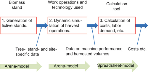
The model comprises three main parts: a stand generator, a dynamic harvest model and a cost calculation model (Figure 1). The stand generator was developed in the Arena simulation package (Kelton et al. 2007; Rockwell Automation 2020), and the resulting stands were visualized in the Heureka software system (SLU 2018). The simulation model for performance analysis was also constructed in Arena, while the calculations of economic profitability were done in an Excel spreadsheet.

Figure 1. Model overview, showing e.g. The interconnections between the three sub-models.

Stand generator

Modelling approaches

Several complex spatiotemporal models have been developed to simulate growth, carbon cycles, biodiversity changes, etc. of forests on a landscape level (Borges et al. 2014; Shifley et al. 2017; Huang et al. 2018; SLU 2018; Linkevičius et al. 2018). Some of these models also include stand level submodels. In North America, the stand simulator FVS (Forest Vegetation Simulator) is used to simulate growth, mortality and regeneration (Crookston and Dixon 2005). In Europe, examples of stand level simulators are SILVA (Pretzsch et al. 2002) and MOSES (Thurnher et al. 2017). Under Nordic conditions, the simulators MOTTI (Hynynen et al. 2005) and Heureka (StandWise) (SLU 2018) are used to study forest-related changes on a stand level. Most stand simulators mentioned above have 3D visualization, and Wang et al. (2009), Kershaw et al. (2010) and Han et al. (2016) present some additional 3D models.

On initialization of stand simulators, distance-independent (e.g. MOTTI (Hynynen et al. 2005)), semi-distance independent (e.g. FVS (Huang et al. 2018)) or distance-dependent (e.g. SILVA (Pretzsch et al. 2002) and MOSES (Thurnher et al. 2017)) individual-tree data are used. Distance-dependent data implies that the position (coordinates) of each tree is required, besides, e.g. species, DBH, height and crown width. Position data can be obtained from field measurements, but that is expensive. An alternative is to use stand generators that position individual trees depending on spatial pattern (e.g. uniform, random or clustered patterns), age, species, width of the crown, etc. (Wang et al. 2009).

Pretzsch (1997) presented a method for positioning trees using the Poisson process approach in combination with restrictions regarding DBH-based stem-to-stem distances, while Valentine et al. (2000) assigned DBH depending on free polygon space around positioned trees. Models using the point process approach have been developed by e.g. Kokkila et al. (2002), using the Gibbs marked point process in which the trees were considered as “charges rejecting each other,” and by Grabarnik and Särkkä (2009) using hierarchical interactions between trees of different sizes. A hierarchical point process approach was also developed by Lister and Leites (2018), while Kershaw et al. (2010) used copulas (multivariate distributions) to generate spatially correlated forest stand structures.

As analyses of spatial patterns and temporal changes were not the primary aim of the present model, a simple stand generator was developed to designate DBH for one tree at a time, calculate height and dry matter content and then randomly position it.

Model

In the model, each stem was assigned a species category and DBH (Figure 2). The total number of stems to be generated was based on estimations of stem density and area of the stand to be cleared.

Figure 2. Input data, model logic and output data for the stand generator (RNG – random number generator, DM – dry matter, DBH – diameter at breast height).

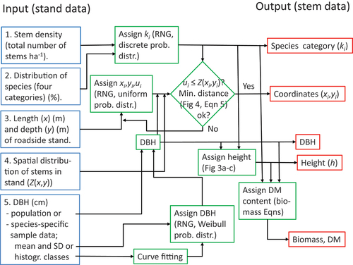
There were four species categories (k) in the model: Scots pine (Pinus sylvestris L.) (k = 1), Norway spruce (Picea abies (L.) Karst.) (k = 2), birch (Betula pendula Roth. and Betula pubescens Ehrh.) (k = 3) and other deciduous trees (k = 4). Each stem was randomly assigned a species category depending on estimations of the actual distribution of species (e.g. in percentages) in the stand to be cleared.

In order to determine the value of DBH (cm) of each stem (when sample data were available, see Figure 2), Weibull distributions were used for each k (Bailey and Dell 1973; Shifley and Lentz 1985; Valentine et al. 2000; Wang et al. 2009). The shape (α) and scale (ß) parameters (α > 0, ß > 0) of the Weibull distribution can be estimated from species-specific sample measurements described by DBH class data in histograms or by data described by the mean ($\bar{x}$) and the standard deviation (s) of DBH. For α = 1, the distribution is the same as the exponential distribution and for α ≈ 3–3.5 the shape of the distribution approximates a normal distribution. By introducing a location parameter (γ), the distribution can be located along the abscissa (γ ≥ 0), i.e. DBH∈Weib(α,ß,γ). As Weibull density functions are in the range [0,+∞], a maximum value of DBH should be used in the model, since very large DBH values may not be probable according to the estimated age of the stand. The maximum value should be chosen with care, however, because too high values (i.e. max DBH >> $\bar{x}$) may bias the outcome of the simulator.

If observed DBH data are grouped in histogram classes, the “Input Analyzer” tool in Arena (Rockwell Automation 2020) can be used to fit Weibull distribution curves to the data. In this tool, the goodness-of-fit are evaluated using the Kolmogorov-Smirnov or Chi-Squared tests (Kelton et al. 2007).

If observed DBH sample data are described only by $\bar{x}$ and s, the following method can be used. The expected value (μ) of a Weibull distribution is described by Equation 1(1) $\mathit{\mu }=\mathit{\beta }\mathrm{\Gamma }\left(1+1/\mathit{\alpha }\right)$(1) (Shifley and Lentz 1985)

(1) $\mathit{\mu }=\mathit{\beta }\mathrm{\Gamma }\left(1+1/\mathit{\alpha }\right)$(1)

where Γ is the gamma function. The variance (σ²) is as follows (Equation 2(2) ${\sigma }^2={\beta }^2\left(\mathrm{\Gamma }\left(1+2/\mathit{\alpha }\right)-{\mathrm{\Gamma }}^2\left(1+1/\mathit{\alpha }\right)\right)$(2) ):

(2) ${\sigma }^2={\beta }^2\left(\mathrm{\Gamma }\left(1+2/\mathit{\alpha }\right)-{\mathrm{\Gamma }}^2\left(1+1/\mathit{\alpha }\right)\right)$(2)

Using Equation 1(1) $\mathit{\mu }=\mathit{\beta }\mathrm{\Gamma }\left(1+1/\mathit{\alpha }\right)$(1) and Equation 2(2) ${\sigma }^2={\beta }^2\left(\mathrm{\Gamma }\left(1+2/\mathit{\alpha }\right)-{\mathrm{\Gamma }}^2\left(1+1/\mathit{\alpha }\right)\right)$(2) , we get Equation 3(3) $\mathit{\mu }/\mathit{\sigma }=\mathit{\hspace{0.17em}}\mathrm{\Gamma }\left(1+1/\mathit{\alpha }\right)/{\left(\mathrm{\Gamma }\left(1+2/\alpha \right)-{\mathrm{\Gamma }}^2\left(1+1/\mathit{\alpha }\right)\right)}^{0.5}$(3) (Shifley and Lentz 1985):

(3) $\mathit{\mu }/\mathit{\sigma }=\mathit{\hspace{0.17em}}\mathrm{\Gamma }\left(1+1/\mathit{\alpha }\right)/{\left(\mathrm{\Gamma }\left(1+2/\alpha \right)-{\mathrm{\Gamma }}^2\left(1+1/\mathit{\alpha }\right)\right)}^{0.5}$(3)

Thus, μ/σ is independent of β, which means that we can calculate the shape parameter (α) using the estimate $\bar{x}$/s = μ/σ in Equation (3)(3) $\mathit{\mu }/\mathit{\sigma }=\mathit{\hspace{0.17em}}\mathrm{\Gamma }\left(1+1/\mathit{\alpha }\right)/{\left(\mathrm{\Gamma }\left(1+2/\alpha \right)-{\mathrm{\Gamma }}^2\left(1+1/\mathit{\alpha }\right)\right)}^{0.5}$(3) , and then obtain β using α and the estimate $\bar{x}$ = μ in Equation (1)(1) $\mathit{\mu }=\mathit{\beta }\mathrm{\Gamma }\left(1+1/\mathit{\alpha }\right)$(1) . However, Equations (1)(1) $\mathit{\mu }=\mathit{\beta }\mathrm{\Gamma }\left(1+1/\mathit{\alpha }\right)$(1) –(3(3) $\mathit{\mu }/\mathit{\sigma }=\mathit{\hspace{0.17em}}\mathrm{\Gamma }\left(1+1/\mathit{\alpha }\right)/{\left(\mathrm{\Gamma }\left(1+2/\alpha \right)-{\mathrm{\Gamma }}^2\left(1+1/\mathit{\alpha }\right)\right)}^{0.5}$(3) ) cannot be solved analytically, but numerical methods must be used (an example of a solver can be found in Weibullfördelningen (2020)).

The height h (m) of each stem of Scots pine, Norway spruce and birch was calculated using second-degree polynomial functions with DBH as the independent variable. These functions were obtained from fitting of averaged DBH class data (0–2 cm, 2–4 cm, etc.) from Marklund (1988), with h = 1.3 m as the vertical intercept (Figure 3). The height function for other deciduous trees (k = 4) was assumed to be the same as for birch (cf. e.g. Johansson (1996) for aspen).

Figure 3. Height of scots pine (upper left), Norway spruce (upper right) and birch (lower) trees with DBH as independent variable. The markers indicate the arithmetic mean in each DBH class (0–2 cm, 2–4 cm, etc.), the bars indicate minimum and maximum values observed (total number of observations n = 396, n = 469 and n = 233, respectively) and the values of R² refer to the curve fitting of arithmetic means (data from Marklund 1988).

The dry matter content in each stem was estimated using the biomass functions of Repola and Ahnlund Ulvcrona (2014) with DBH and h as independent variables. For other deciduous trees (category 4), the biomass functions of Johansson (1999) were used with DBH as the only independent variable.

The preliminary coordinates of a specific stem i (x_i,y_i) were determined in a Cartesian coordinate system, using uniform random distributions with constant probabilities between the endpoints of the stand surface. For a rectangular surface, for example, the surface can be delimited by the coordinates (x_min,y_min), (x_min,y_max), (x_max,y_max) and (x_max,y_min). A third random number u_i was also generated from a uniform distribution (u_i∈Unif(0,1)) as a test number (Pretzsch 1997). If u_i ≤ Z(x_i,y_i), the position (x_i,y_i) of the stem was approved preliminarily. The function Z(x_i,y_i) is a continuous probability distribution (0 ≤ Z(x_i,y_i) ≤ 1) describing the probabilities of trees being located in e.g. clusters and strips (Pretzsch 1997). If u_i > Z(x_i,y_i), new sets of position parameters {x_i,y_i,u_i} are generated until u_i ≤ Z(x_i,y_i).

If the stems are to be distributed within a strip-shaped surface (Z_S(x_i,y_i)), the following expression (Equation 4(4) $Z_S\left(\mathit{x},\mathit{y}\right)=e^{-\left(cos\alpha (x-X_M\right)+sin\mathit{\alpha }\left(\mathit{y}-Y_M\right){)}^4/E^2}$(4) ) can be used (Pretzsch 1997)

(4) $Z_S\left(\mathit{x},\mathit{y}\right)=e^{-\left(cos\alpha (x-X_M\right)+sin\mathit{\alpha }\left(\mathit{y}-Y_M\right){)}^4/E^2}$(4)

where α (rad) is the angle between the longitudinal direction of the stand and the y-axis, (X_M,Y_M) describes the location of the center point of the stand, and E is an intensity factor determining strip width (Pretzsch 1997). Visual examples of strip-shaped stands using Equation 4(4) $Z_S\left(\mathit{x},\mathit{y}\right)=e^{-\left(cos\alpha (x-X_M\right)+sin\mathit{\alpha }\left(\mathit{y}-Y_M\right){)}^4/E^2}$(4) are shown in Nilsson et al. (2020). For simplification, a continuous probability distribution without variations in the y-direction (depth of the stand) can be used in practice, based on data from sample areas (Nilsson et al. 2020).

Studies on the distance between stems of spontaneously grown brushwood, and its dependence on DBH under Swedish conditions, are lacking in the literature. Therefore, results from a German investigation (Pretzsch 1997) were used to determine the minimum stem distances allowed in the stand generator. Based on data from stands with totally around 5,000 larch and beech trees, Pretzsch (1997) suggested 1-percentile curve-fitted equations in which the distance was dependent on DBH of the trees. The 1-percentile equations implied that 99% of the trees had a longer distance to the nearest neighboring tree of a specific species. These fits were obtained from DBH-data in the ranges 20–70 cm (larch-larch and larch-beech) and 5–70 cm (beech-beech). In the present stand generator, second-degree polynomial equations were fitted to Pretzsch (1997) data in order to get more reasonable equations when extrapolating to DBH = 0 (Figure 4). The resulting minimum distances allowed in the model between coniferous trees (D_c–c), between deciduous trees (D_d–d) and between coniferous and deciduous trees (D_c–d,), or vice versa (D_d–c) (c for k = {1,2}, d for k = {3,4}), are presented in Figure 4.

Figure 4. Minimum distances between coniferous trees (D_c-c), coniferous and deciduous trees (D_c-d) (or vice versa (D_d-c)) and deciduous trees (D_d-d) used in the stand generator. The marks show the 1-percentile stem-to-stem distances of totally around 5000 larch and beech trees (data from Pretzsch (1997)).

For each new tree j of species category k_j, the distances d to trees already positioned were calculated in the stand generator. If the distance d_i–j to a neighboring tree i of species category k_i was shorter than the minimum distance allowed, i.e. (Equation 5(5) $d_{\mathit{i}-\mathit{j}}\le \mathit{\hspace{0.17em}}\mathrm{Max}\left[D_{\mathit{ki}-\mathit{kj}}\left(\mathit{DB}{H}_i\right),D_{\mathit{kj}-\mathit{ki}}\left(\mathit{DB}{H}_j\right)\right],$(5) ),

(5) $d_{\mathit{i}-\mathit{j}}\le \mathit{\hspace{0.17em}}\mathrm{Max}\left[D_{\mathit{ki}-\mathit{kj}}\left(\mathit{DB}{H}_i\right),D_{\mathit{kj}-\mathit{ki}}\left(\mathit{DB}{H}_j\right)\right],$(5)

new sets of position parameters {x_i,y_i,u_i} were generated; otherwise, the position was approved.

Harvest model

The stands were assumed to have a base station to/from which the machine arrives/leaves the stand. The machine then fells all the intended trees through a series of repositions in the area. At each position, the machine fells the trees within reach and places them in a pile and then repositions for further felling.

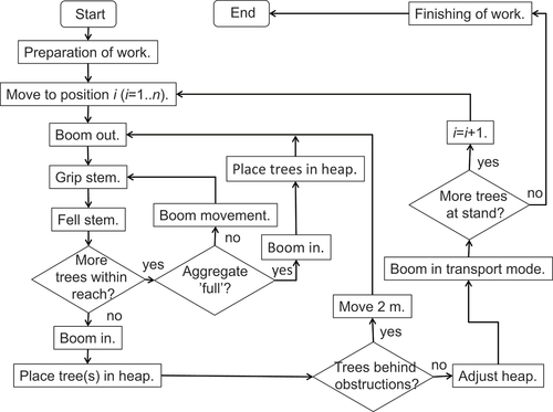
The model boom cycle consists of the following work elements (time consumption in parenthesis): boom out (t_b.out), grip stem (t_grip), cut stem (t_cut), move boom to next stem (t_b.move), grip stem (t_grip), etc. until the felling head was “full” or there were no more trees to be cut, and boom in (t_b.in) (Figure 5). The work element “boom out” started when the boom moved out after the machine had moved to a new position or when the stems had been dropped in a pile, and ended when the felling head touched a new stem to be cut. The work element “boom in” started when the boom was moved toward the machine and ended when the stems in the head were dropped in a pile.

Figure 5. Flowchart for harvester operations.

In order to calculate the time consumption for boom movements, Eliasson (1999), followed by e.g. Sängstuvall et al. (2012), Jundén et al. (2013) and Berg et al. (2014), used equations of the type (Equation 6(6) $t_{\mathit{boom}}=\mathit{\hspace{0.17em}}{C}_{\mathit{boom}}+\mathrm{Max}\left[\left(C_r+\mathit{L}/\mathit{v}\right),\left(C_a+\mathit{a}/\mathit{\omega }\right)\right]$(6) ):

(6) $t_{\mathit{boom}}=\mathit{\hspace{0.17em}}{C}_{\mathit{boom}}+\mathrm{Max}\left[\left(C_r+\mathit{L}/\mathit{v}\right),\left(C_a+\mathit{a}/\mathit{\omega }\right)\right]$(6)

where C_boom is a constant (s) and the second term the maximum time for radial or angular movements. C_r and C_a are constants (s), L (m) and a (rad) describe distances and v (m s⁻¹) and ω (rad s⁻¹) are linear and angular velocities, respectively. Eliasson (1999), Sängstuvall et al. (2012) and Jundén et al. (2013) used the following values: C_boom = 1.5 s, C_r = 0.1 s, C_a = 0.1 s, v = 2.5 m s⁻¹ and ω = 0.35 rad s⁻¹. In the present study, it was assumed that t_b.out = 4 s (Equation 6(6) $t_{\mathit{boom}}=\mathit{\hspace{0.17em}}{C}_{\mathit{boom}}+\mathrm{Max}\left[\left(C_r+\mathit{L}/\mathit{v}\right),\left(C_a+\mathit{a}/\mathit{\omega }\right)\right]$(6) ), based on a radial movement with L = 6 m (on average) and C_boom = 1.5s, C_r = 0.1 s and v = 2.5 m s⁻¹. The average time to move the head to a new tree (t_b.move) was also based on Equation 6(6) $t_{\mathit{boom}}=\mathit{\hspace{0.17em}}{C}_{\mathit{boom}}+\mathrm{Max}\left[\left(C_r+\mathit{L}/\mathit{v}\right),\left(C_a+\mathit{a}/\mathit{\omega }\right)\right]$(6) and the assumption that L = 1.0 m, which resulted in t_b.move = 2 s. In different studies, the value of t_b.in has varied from t_b.in ≈ t_b.out (Nilsson 2009; Sängstuvall et al. 2012) up to t_b.in = 1,4t_b.out (Edlund 2009). In the present study, it was assumed that t_b.in = 5s. The time consumption for gripping and cutting a stem with area A was t_grip + t_cut = 1 + A/800, where the first term (1s) is a constant (Eliasson 1999) and where 800 cm² s⁻¹ is the cutting speed (Eliasson 1999; Sängstuvall et al. 2012). For simplicity, it was assumed that A was calculated with a radius r = DBH/2.

The harvester had a crane with an accumulating felling head. The maximum volume of trees in the felling head depends on a large number of factors such as the design and storage capacity of the head, the DBH, height, crown spread and spatial density of the trees, and the driver’s experience and skill. In three harvester performance studies, Iwarsson Wide (2009b, 2009c, 2009d) found that the average number of trees in each boom cycle was 4.3, 3.6 and 1.3, while the average values of DBH were 4.0, 6.2 and 9.9 cm, respectively. Multiplying the average number of trees with the average DBH results in 17.2, 22.3 and 12.9 cm, and calculation of the average cross-sectional area (at DBH) results in 54, 109 and 100 cm², respectively. Based on these results, it was assumed in the model that the head was full when the sum of the stems’ DBH exceeded 20 cm or when the total cross-sectional area of the stems (at DBH) exceeded 100 cm².

The machine speed between harvest positions was 1.11 m s⁻¹ (4 km hr⁻¹) and the acceleration and deceleration 0.19 m s⁻² (2500 km hr⁻²), which approximately correspond to the data used by Eliasson (1999). The distance between machine positions was dependent on maximum boom reach, harvest depth in the stand and distance to the nearest tree to be felled (Figure 6).

Figure 6. Machine and boom movements.

Some time (t_arrange) may be needed to arrange stems in the pile before moving the machine. Furthermore, when clearing brushwood, it is often necessary to clear shrubs and thin trees not used for fuel purposes. The time needed for this operation (t_clear) may differ considerably among stands (Iwarsson Wide 2009a). In a base scenario simulated, it was assumed that t_clear = 0 and t_arrange = 5 s (per pile).

In some cases there may be trees that should be left in the stand, e.g. due to their conservation value. Such trees, as well as light poles and boulders, are examples of obstructions for the boom movements. In the model, data on position and width of obstacles can be used to identify possible obstructed trees (Nilsson et al. (2020). The time needed to relocate the harvester to reach obstructed trees was assumed to correspond to the time of moving the machine 2 m.

Work schedules were specified in the model regarding e.g. daily starting and finishing time and time and duration of lunch. During nights, the machine was parked at the stand center.

In the cost calculations, the working time from the simulations were recalculated from productive machine hours (PMh) to scheduled machine hours (SMh) with a factor of 1.53 (Kuitto et al. 1994). The hourly cost of the harvester was €116 and the relocating cost €192 per harvesting site (Nilsson et al. 2020) (an exchange rate of 10.4 SEK €⁻¹ was used in the paper).

Verification and validation processes

Verification

The stand generator and the harvest model were verified by following the flow of entities through the so-called SIMAN blocks, which form the basic structure of Arena (Kelton et al. 2007). This was done manually and with the help of the tools (“watch,” “highlight active module,” etc.) available in Arena for different scenarios and extreme cases. In addition, the models were verified by animating the simulations. By studying in detail what happens during the simulations graphically on the screen, the models’ work was analyzed step by step and unintended programming errors were detected. After the verifications, the models were considered to work with sufficient reliability.

Validation

Two field studies of harvesting brushwood along roadsides were chosen to validate the models since relatively accurate data are available on both stand characteristics and harvest operations; the study by Iwarsson Wide (2009b) and the study by Edlund (2009). The validations are presented in detail by Nilsson et al. (2020).

In the study by Iwarsson Wide (2009b), trees were cleared along a roadside in Jämtland in Sweden with a Valmet 911 equipped with a Bracke C16.a accumulating head. The length of the studied roadside was 240 m and the clearing depth 7 m. The number of trees, species, DBH and height in plots of 1.0 m width at every 15 m of the roadside were recorded before harvest (the total number of trees in these plots was 163, with birch as the most common species category (54%)). In the validation, the number of stems in each plot was used to construct a continuous probability distribution (Z(x_i,y_i)) for this distance (see Nilsson et al. (2020)). The total number of trees felled was 1174, corresponding to a tree density of 6990 stems ha⁻¹. As data on DBH for each stem in the plots were available, the Weibull-parameters for each species category were obtained using a curve-fitting tool in Arena.

In the field study by Edlund (2009) (reanalyzed in a recent paper by Fernandez-Lacruz et al. (2021)), the trees were felled along a forest road near Örnsköldsvik in Sweden. A Rottne H8 single grip harvester with a Naarva-grip 1500–25 EH accumulating harvester head was used. The Weibull parameters β and α used in the stand generator were obtained using values of mean $\bar{x}$ and standard deviation s (Edlund 2009; Nilsson et al. 2020) and a numerical solver (Weibullfördelningen 2020). The value of γ was set to 0 and a maximum value of 25 cm was used to avoid extreme DBH-values (the age of the stand was estimated to around 30 years (Edlund 2009)). Since no species-specific data were available, it was assumed that the coniferous trees were represented by Scots pine and that the deciduous trees were represented by birch, and that the statistical data on DBH (mean and standard deviation) were the same for these species. It was also assumed that there were no gaps and felling obstacles in the stand as no data were available. Ten replications were generated, and the replication (stand) with DBH values (mean and SD) closest to observed mean and SD values was used in the validation.

Generation of stand types

Twenty-nine stand types with a spatial length of 25 m and a depth of 5 m were generated (Table 1). For all stand types, it was assumed that they contained on average 30% pine, 5% spruce and 65% birch, and that the maximum DBH was 30 cm. It was also assumed that these stands had no harvest obstacles such as light poles or boulders. Each stand type was characterized by three parameters: average DBH, standard deviation of DBH, and number of stems per hectare. For each stand, a number of simulation replications were run with the stand generator until a representative stand was found with an average DBH and standard deviation within ±0.05 cm of the targeted values (Table 1). The number of replications to reach the targeted values was dependent on the number of trees in each stand and varied from about 10 to 300. Mean basal area-weighted DBH and total dry matter content of the simulated stand types are presented in Table 1. The stands were visualized in Heureka (Figure 7).

Figure 7. Visualization in Heureka of stand types 4.0/3.0/25 (left) and 7.0/4.0/150 (right), with a total dry matter content in stems and branches of 134 kg and 2361 kg, respectively (table 1).

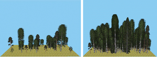
Table 1. Characteristics for the 29 stand types (25 m × 5 m) generated. The stands can be identified by the three parameters p₁/p₂/p₃, where p₁ is targeted average DBH (cm), p₂ targeted standard deviation of DBH (cm) and p₃ targeted number of stems in hundreds per hectare (100 ha^−1.).

Stand type	Simulated representative
	Number of stems	DBH, average (cm)	DBH, standard dev. (cm)	Mean basal area-weighted DBH (cm)	Total dry matter content (kg)
4.0/3.0/25 4.0/3.0/50 4.0/3.0/75 4.0/3.0/100 4.0/3.0/150 4.0/3.0/200 4.0/4.5/25 4.0/4.5/50 4.0/4.5/75 4.0/4.5/100 4.0/4.5/150 4.0/4.5/200 7.0/4.0/25 7.0/4.0/50 7.0/4.0/75 7.0/4.0/100 7.0/4.0/150 7.0/5.0/25 7.0/5.0/50 7.0/5.0/75 7.0/5.0/100 7.0/5.0/150 10.0/5.0/25 10.0/5.0/50 10.0/5.0/75 10.0/7.0/25 10.0/7.0/50 10.0/7.0/75 10.0/7.0/0.3	31 63 94 125 188 250 31 63 94 125 188 250 31 63 94 125 188 31 63 94 125 188 31 63 94 31 63 94 4	3.97 3.97 3.98 3.97 3.98 3.98 3.95 4.00 3.95 4.00 4.02 3.99 7.05 7.00 7.05 6.97 6.96 6.98 6.96 6.98 6.96 6.98 9.97 9.97 9.97 9.95 9.98 9.98 9.98	3.00 2.99 2.99 2.97 2.98 3.02 4.51 4.48 4.50 4.52 4.46 4.48 3.97 3.95 4.03 3.97 4.05 4.97 5.00 5.00 4.95 4.98 4.97 4.99 5.02 6.96 6.97 7.02 6.98	8.2 7.9 7.8 8.0 8.0 8.2 12.7 14.9 13.6 13.6 12.4 13.6 10.7 11.0 11.4 11.1 11.1 13.6 13.2 13.1 13.4 13.4 13.8 14.2 14.9 19.1 18.8 18.4 16.4	134 275 413 546 825 1,095 223 432 673 903 1,328 1,727 393 796 1,187 1,558 2,361 453 936 1,404 1,814 2,723 789 1,591 2,367 933 1,826 2,876 108

The harvest of stems was simulated for 10 consecutive stands (i.e. 250 m) of each type to reduce edge effects, and resulting performance then divided by 10. The maximum value of BL_x was 5.5 m (Figure 6) and the distance between harvester and stand surface a maximum of 2 m. Movements between machine positions and movement back to the original position at the stand were included in the simulations. No other transports were simulated. As the harvest model was non-stochastic, the harvest of each stand type (250 m) was simulated once.

Results

Validations

For the Iwarsson Wide (2009b) study, the simulated and observed stand characteristics were quite similar (Table 2). The number of machine positions and boom cycles were also similar. Regarding time consumption and productivity, the simulations showed more favorable results than were observed by Iwarsson Wide (2009b) (Table 2). One probable reason was that the share of total number of boom cycles with few stems was higher in the field study (Figure 8), although the stand was quite young with relatively small DBH values. Furthermore, Iwarsson Wide (2009b) noted that the machine also cut stems shorter than breast height (DBH = 0) as there, in addition, was a need of clearing such vegetation. When boom cycles with less than three stems were omitted in the field study, the simulated and observed productivities were more conformable (Table 2).

Figure 8. Simulated and observed (Iwarsson Wide 2009b) number of stems in the boom cycles.

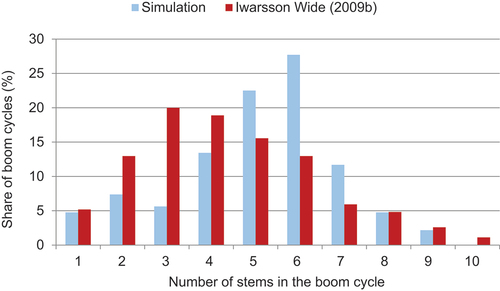
Table 2. Simulated and observed (Iwarsson Wide 2009b) stand and harvest performance data.

Stand and machine performance criteria	Simulated	Observed
Stand
Mean DBH (standard dev.)	4.1 (2.6)	4.1 (2.7)
Stem density (ha^−1)	6990	6990
Total biomass quantity (tonnes of DM)	4.83	4.64^a
Machine performance
Number of machine positions	28	29
Number of boom cycles	231	270^b/221^c
Time consumption
Boom out (min)	15.4	116.6^b,d/103.9^c,d
Grip and fell (min)	20.0
Boom movement to next stem (min)	25.2
Boom in (min)^e	21.6	22.1^b/18.8^c
Movements (min)	7.4	4.9
Total (min)	8.9	143.6^b/127.6^c
Productivity (PMh ha^−1)	8.9	14.2^b/12.6^c
Productivity (tonnes DM PMh^−1)	3.2	1.9^b/2.2^c

^aBased on measurements in the 17 study plots.

^bResults when there were at least one stem in the boom cycle.

^cResults when there were at least three stems in the boom cycle.

^dIncludes work elements “boom out,” “grip and fell” and “boom movement to next stem.”

^eIncludes work element “fix pile.”

For the Edlund (2009) study, the simulated time consumption and productivity was consistent with observed values (Table 3), although the simulated performance was somewhat higher. The DM-related productivity differed, but it can be noted that the simulated DM values were based on Repola and Ahnlund Ulvcrona’s (2014) biomass model, and that the observed values were based on Ulvcrona’s biomass model (Edlund 2009) and on weighed and oven-dried chips three months after felling (Edlund 2009).

Table 3. Simulated and observed (Edlund 2009) performance data for clearing of brushwood at a roadside (150 m x 2.5 m) near Örnsköldsvik in Sweden.

Performance criteria	Simulated	Observed
Time consumption
Boom out (min)	7.4	9.0
Accumulation (min)	25.1	25.9
Boom in (min)	10.8	12.6
Movement (min)	4.8	4.3
Total (min)	48.0	51.8
Total (PMh ha^−1)	21.3	23.0
Number of boom cycles	111	103
Quantity harvested (t DM)	3.99	4.93^a/3.65b^b
Machine performance (PMh t^−1 DM)	0.20	0.18^a/0.24^b

^aEstimated dry matter content of trees according to the Ulvcrona biomass model (Edlund 2009).

^bCalculated (weighed and oven-dried) dry matter content of harvested chips.

Based on these two studies (Iwarsson Wide 2009b; Edlund 2009), it was concluded that the stand generator and the harvest model can be considered suitable for the purpose of the study.

Performance analysis

As expected, total time required for harvesting the stand types varied depending on the number of stems harvested (Figure 9). For stands with thin and dense stems, the task “move to next stem” took the longest, while the task “boom in” was the most time-consuming for stands with thicker stems. The number of machine positions varied from 20 to 23 (when simulating 10 stands in a row) and the total time for movement therefore only differed a little between the stand types. For the very sparse stand (10.0/7.0/0.3), however, “moving” accounted for more than half of the total time consumption (Figure 9).

Figure 9. Productive time (PMh per 25 m) required for the different tasks when harvesting the stands investigated.

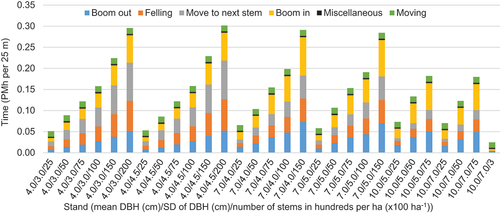
The more stems of a certain diameter that a harvester head accumulated when cutting, the higher the simulated productivity. The average number of stems per boom cycle varied from 1.4 to 5.8, decreasing with higher average DBH.

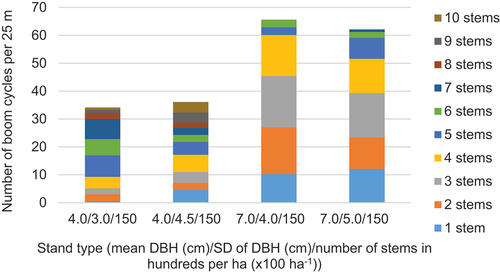
The number of boom cycles varied greatly, even for stands with the same stem density. For the stands 7.0/4.0/150 and 7.0/5.0/150 there were no boom cycles with more than six and seven stems, respectively, while the number of stems in each boom cycle was more distributed for the two stands with smaller stems (Figure 10). Since the number of stems in the boom cycles was dependent on assumptions made in the simulations, a sensitivity analysis was made to analyze the influence of maximum accumulating volume of the head (see below).

Figure 10. Number of boom cycles, broken down by number of stems in each cycle, for four stands with the same stem density (15,000 stems ha⁻¹).

The performance, expressed in tonnes of DM per PMh, was strongly dependent on DBH and density of the stems (Figure 11; base scenario). At approx. 10,000 stems ha⁻¹, however, the performance flattened out, while an increased diameter of the trees was always beneficial. The very sparse stand (10.0/7.0/0.3) contained a large birch with DBH = 19.5 cm, but despite a large timber yield the performance was relatively low (Figure 11), partly due to that a lot of time, relatively speaking, was required for movements (Figure 9).

Figure 11. Productivity (in tonnes DM per PMh) for the base scenario (upper, left), and change in productivity using a 30% longer boom (upper, right), an increased aggregate volume capacity by 30% (lower, left) and both a 30% longer boom and increased volume capacity (lower, right). The stand types are denoted by: average DBH/standard deviation of DBH.

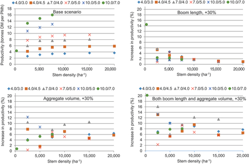
Sensitivity analyses showed that increasing the length of the boom by 30% increased the average performance (all stand types included) by 2.6%. For sparse stands (up to approx. 5,000 stems/ha), the picture was more fragmented (Figure 11). This can probably be explained by random variations in stem positions, as this diversity in performance was more pronounced the fewer trees were in the stands (but note that it is a matter of single percentage points of difference). In general, however, longer boom reach had less importance the denser the stems were.

An increase in the maximum volume capacity of the harvester head by 30% increased performance by an average of 5.9% (all stands included). Based on Figure 11, however, there were no clear correlations between increased performance and stem density/average (arithmetic) DBH. In simulations with both 30% longer boom and 30% larger accumulating volume capacity, performance increased by an average of 8.8% (Figure 11). There were synergistic effects of these measures for the sparse stands (300 and 2,500 stems/ha), i.e. the performance increase was greater when both measures were implemented simultaneously compared to summing the performance increases for the measures separately.

Cost calculations

Felling costs differed markedly between the different types of stands, both with regard to cost per 25 m-piece and per harvested amount of DM (Figure 12). The simulations showed a clear relationship between cost and the number of stems felled. For the same stem densities, however, there was only a small effect of DBH where costs increased with increasing DBH.

Figure 12. Harvest costs in € per 25 m and in € per tonne of DM for the stands investigated (relocating costs not included).

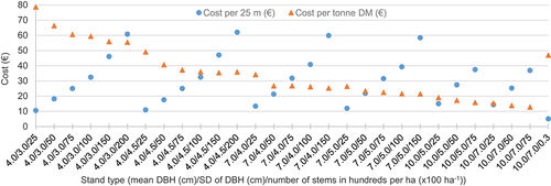
The cost per tonne of dry matter was governed by a combination of tree size and number of trees felled (lowest cost when felling a large number of thicker stems and vice versa). Costs per tonne of DM were, in comparison to 25 m-piece costs, to a smaller degree influenced by stem density. This effect was clear for all type stands except for stands with low DBH and low SD of DBH, i.e. stands with lower standing volume.

Average DBH had a decisive role for the costs per tonne of DM (Figure 12). For example, the cost for the stand 7.0/5.0/100 was 40% lower than for the stand 4.0/4.5/100. Increasing standard deviations of DBH, while keeping the stem density and average DBH constant, also resulted in a lower cost per tonne of DM (Figure 12), following the expected pattern of a negative correlation between harvesting costs per tonne of DM and average volume of trees harvested.

Discussion

Since there is a large number of variations on the characteristics of a brushwood stand, a stand generator was constructed to enable simulation experiments on arbitrary stand configurations. The stand generator in this study, however, does not explicitly consider hierarchical interactions such as asymmetric competition, i.e. that large trees influence the presence and growth of small trees but not vice versa (Grabarnik and Särkkä 2009). Furthermore, the relationship between DBH and height is more complex (Sharma and Breidenbach 2014) than assumed in this study; in fact allometric factors such as height, crown length and crown width rather determine DBH than vice versa (Söderberg 1986). Having these limitations in mind, the present stand generator was considered to produce realistic results according to the purpose of the study.

To validate the harvest model, only two field studies with sufficient data for harvest of brushwood along roadsides were found. Thus, no statistical tests were carried out for deeper analyses. However, the verification and validation showed that the harvest simulation model can be considered reliable, although there were uncertainties considering e.g. the time spent for clearing of small stems that yield negligible amounts of fuel. In field studies, the driver’s experience, skill and daily state can also play an important role. Fernandez-Lacruz et al. (2013) refer to some studies (Kärhä et al. 2004; Purfürst and Erler 2011; Purfürst and Lindroos 2011) which have shown that there can be large differences in productivity among drivers. Regardless of these uncertainties, the developed model can be of use in comparative studies, where analyses of relative changes are of greater importance than absolute figures on performance and time consumption. The model can also be used to evaluate new harvest strategies and technologies, as input data easily can be changed. However, the most time-consuming part in simulation often is collection of reliable input data. On the contrary, the time to simulate the harvest of the stand types in this study only took about ten seconds (with no animation).

In this study, the work of a harvester was simulated. In such harvesting systems, a forwarder is needed for transport of the stems. In some cases the dual-purpose harwarder machine may be more competitive due to lower total relocation costs. In a study by Laitila and Väätäinen (2021), one-machine configurations generally had lower costs than two-machine configurations when the harvested volumes were less than about 100 m³ at each harvesting site, otherwise two-machine configurations were more competitive. However, when the harvested trees were small (less than about 15 dm³ each), harwarders were more competitive also at large volumes (about 100 m³) at each site. In this case, the relocation cost was €174, the number of trees per ha was 6,000 and the forwarding distance was 250 m (Laitila and Väätäinen 2021). In our study, the 25 m stand with the lowest costs (10.0/7.0/75) (Figure 12) had an approximate volume of 6 m³ (2.9 tonnes of DM (Table 1), assuming a density of 0.5 tonnes of DM per m³). This indicates that a harwarder machine is an interesting alternative, which should be investigated in future simulation studies.

In the case of brushwood harvesting, it is important to consider indirect benefits such as increased revenues or reduced costs in the future. Clearing along roads will increase visibility, ensure safe passage for traffic and prolong the roads’ lifespan by providing better drainage conditions to the road banks (Fernandez-Lacruz et al. 2021). Careful clearing in the rural landscape also benefits biodiversity, although the effect is dependent on the composition of the surrounding landscape (Ebenhard et al. 2017; de Jong et al. 2017). Unfortunately, the quantification and monetary valuation of such effects often is subject to great uncertainty, causing underestimations of the benefits created (Grönlund 2020). However, this should not be grounds for ignoring them.

The simulations of different stand types provide a data basis for the users of the calculation tool that has been developed in the project (see skogforsk.se). By combining different 25 m pieces and then adding user-appropriate values (hourly costs, relocation cost, transport distance, etc.) into the calculation tool, performance and costs for the case in question can be estimated. Lack of detailed data on the actual stand to be harvested may make it difficult to choose the most appropriate stand types. However, by starting from pictures and simple descriptions of the stand types (density, average DBH, etc.) (Nilsson et al. 2020), one should still be able to get a reasonably accurate estimation of how large the costs will be. Since relatively many stand types have been developed (in this case for roadside clearing), there are also opportunities to choose different similar stand types and conduct a sensitivity analysis. Thus, the user of the calculation tool can get a sense of how performance and costs may vary in reality.

Conclusions

This paper presents a model which uses data that can be obtained relatively easily to simulate brushwood stands and time consumption when harvesting those stands. The validations showed that the model can produce realistic results according to its purpose. Thus the model can be used to determine whether harvesting operations will be profitable or not, thereby addressing a main challenge in these operations with often low profitability. Reducing risk of negative profitability is a key factor for long-term increased brushwood harvest.

Acknowledgements

The authors would like to express gratitude to Maria Iwarsson Wide, Skogforsk, Sweden, for providing model validation data and for helpful discussions.

Disclosure statement

No potential conflict of interest was reported by the author(s).

Additional information

Funding

This research was funded by the Swedish Farmers´ Foundation for Agricultural Research, grant number [O-17-21-988].

References

- Bailey RL, Dell TR. 1973. Quantifying diameter distributions with the Weibull function. For Sci. 13(3–4):195–203. Cited by: Shifley S, Lentz E. 1985. Quick estimation of the three-parameter Weibull to describe tree size distributions. For Ecol Manage. 13:195-203. doi: 10.1016/0378-1127(85)90034-9.
- Berg S, Bergström D, Nordfjell T. 2014. Simulating conventional and integrated stump- and round-wood harvesting systems: a comparison of productivity and costs. Int J For Eng. 25(2):138–155. doi: 10.1080/14942119.2014.941640.
- Bergström D, Fernandez-Lacruz R, Forsman M, Lundbäck J, Nilsson Å, Bredberg C. 2015. Slutrapport, Skog, Klimat & Miljö - ett projekt i Norr- och Västerbotten 2012–2014 [Final report, Forestry, Climate & Environment – a project in Norr- and Västerbotten 2012–2014]. Umeå (Sweden): Länsstyrelsen Västerbotten. Swedish.
- Borges JG, Nordström EM, Garcia-Gonzalo J, Hujala T, Trasobares A (Eds.). 2014. Computer-based tools for supporting forest management. The experience and the expertise world-wide. Umeå: Swedish University of Agricultural Sciences. Report of Cost Action FP 0804 Forest Management Decision Support Systems (FORSYS). ISBN: 978-91-576-9236-8.
- Crookston NL, Dixon GE. 2005. The forest vegetation simulator: a review of its structure, content, and applications. Comput Electron Agric. 49(1):60–80. doi: 10.1016/j.compag.2005.02.003.
- Dániel-Ferreira J. 2021. Linear infrastructure habitats for the conservation of plants and pollinators. The value of road verges and power-line corridors for landscape-scale diversity and connectivity [ dissertation]. Acta Universitatis Agriculturae Sueciae 2021:63, Uppsala: Swedish University of Agricultural Sciences.
- de Jong J, Akselsson C, Egnell G, Löfgren S, Olsson BA. 2017. Realizing the energy potential of forest biomass in Sweden – how much is environmentally sustainable? For Ecol Manage. 383:3–16. doi: 10.1016/j.foreco.2016.06.028.
- Ebenhard T, Forsberg M, Lind T, Nilsson D, Andersson R, Emanuelsson U, Eriksson L, Hultåker O, Iwarsson Wide M, Ståhl G. 2017. Environmental effects of brushwood harvesting for bioenergy. For Ecol Manage. 383:85–98. doi: 10.1016/j.foreco.2016.05.022.
- Edlund M. 2009. Produktivitet och lönsamhet vid skogsbränsleuttag längs skogsbilvägar [Productivity and profitability of forest fuel harvest in forest roads’ right of way]. Umeå (Sweden): Swedish University of Agricultural Sciences. Arbetsrapport 243. Swedish.
- Eliasson L. 1999. Simulation of thinning with a single-grip harvester. For Sci. 45(1):26–34.
- Emanuelsson U, Ebenhard T, Eriksson L, Forsberg M, Hansson P-A, Hultåker O, Iwarsson Wide M, Lind T, Nilsson D, Ståhl G, et al. 2014. Landsomfattande slytäkt – potential, hinder och möjligheter [Small trees and bushes – potential, barriers and opportunities]. Uppsala: SLU Swedish Biodiversity Centre; [accessed 2022 Aug 16]. https://www.slu.se/globalassets/ew/org/centrb/cbm/dokument/ovrig-forskning/huvudrapport-sly-stem.pdf. Swedish.
- Fernandez-Lacruz R, Di Fulvio F, Bergström D. 2013. Productivity and profitability of harvesting power line corridors for bioenergy. Silva Fenn. 47(1). article id 904. doi: 10.14214/sf.904.
- Fernandez-Lacruz F, Edlund M, Bergström D, Lindroos O. 2021. Productivity and profitability of harvesting overgrown roadside verges – a Swedish case study. Int J For Eng. 32(1):19–28. doi: 10.1080/14942119.2020.1822664.
- Grabarnik P, Särkkä A. 2009. Modelling the spatial structure of forest stands by multivariate point processes with hierarchical interactions. Ecol Model. 220(9–10):1232–1240. doi: 10.1016/j.ecolmodel.2009.02.021.
- Grönlund Ö 2020. Forest operations in multifunctional forestry [ dissertation]. Acta Universitatis agriculturae Sueciae 2020:61, Uppsala: Swedish University of Agricultural Sciences.
- Han Y-Y, Wu B-G, Wang K-Y, Guo E-Y, Dong C, Wang Z-B. 2016. Individual-tree form growth models of visualization simulation for managed larix principis-rupprechtii plantation. Comput Electron Agric. 123:341–350. doi: 10.1016/j.compag.2016.03.009.
- Huang S, Ramirez C, McElhaney M, Evans K. 2018. F3: simulating spatiotemporal forest change from field inventory, remote sensing, growth modeling, and management actions. For Ecol Manage. 415(2):26–37. doi: 10.1016/j.foreco.2018.02.026.
- Hynynen J, Ahtikoski A, Siitonen J, Sievänen R, Liski J. 2005. Applying the MOTTI simulator to analyse the effects of alternative management schedules on timber and non-timber production. For Ecol Manage. 207(1):5–18. doi: 10.1016/j.foreco.2004.10.015.
- Iwarsson Wide M. 2009a. Skogsbränsleuttag i vägkanter – prestationsstudie, uttag av skogsbränsle i vägkant med ponsse dual med EH25 [recovery of forest fuel along forest road – productivity study. Recovery of forest fuel along forest road with ponsse dual with EH25]. Uppsala (Sweden): Skogforsk. Arbetsrapport 2009:696. Swedish.
- Iwarsson Wide M. 2009b. Skogsbränsleuttag i vägkanter – Prestationsstudie. Uttag av skogsbränsle i vägkant med Bracke C16 [Recovery of forest fuel along forest road – Productivity study. Recovery of forest fuel along forest road with Bracke C16]. Uppsala (Sweden): Skogforsk. Arbetsrapport 2009:695. Swedish.
- Iwarsson Wide M. 2009c. Skogsbränsleuttag med Bracke C16. Bränsleuttag med Bracke C16 i tall- respektive barrblandskog [recovery of forest fuel with Bracke C16. Recovery of forest fuel in pine and mixed coniferous forests with Bracke C16]. Uppsala (Sweden): Skogforsk. Arbetsrapport 2009:682. Swedish.
- Iwarsson Wide M. 2009d. Teknik och metod Ponsse EH25. Trädbränsleuttag med Ponsse EH25 i kraftledningsgata [Technique and method Ponsse EH25.Wood fuel recovery with Ponsse EH25 in power line corridor]. Uppsala (Sweden): Skogforsk. Arbetsrapport 2009-681. Swedish.
- Johansson T. 1996. Site index curves for European aspen (populus tremula L.) growing on forest land of different soils in Sweden. Silva Fenn. 30(4):437–458. doi: 10.14214/sf.a8503.
- Johansson T. 1999. Biomass equations for determining fractions of European aspen growing on abandoned farmland and some practical implications. Biomass Bioenerg. 17(6):471–480. doi: 10.1016/S0961-9534(99)00073-2.
- Jundén L, Bergström D, Servin M, Bergsten U. 2013. Simulation of boom-corridor thinning using a double-crane system and different levels of automation. Int J For Eng. 24(1):16–23. doi: 10.1080/14942119.2013.798131.
- Kelton WD, Sadowski RP, Sturrock DT. 2007. Simulation with Arena. 4th ed. Boston, USA: McGraw-Hill.
- Kershaw JA Jr, Richards EW, McCarter JB, Oborn S. 2010. Spatially correlated forest stand structures: a simulation approach using copulas. Computers And Electronics In Agriculture. 74(1):120–128. doi: 10.1016/j.compag.2010.07.005.
- Kokkila T, Mäkelä A, Nikinmaa E. 2002. A method for generating stand structures using Gibbs marked point process. Silva Fenn. 36(1):265–277. doi: 10.14214/sf.562.
- Kuitto PJ, Keskinen S, Lindroos J, Oijala T, Rajamäki J, Räsänen T, Terävä J. 1994. Puutavaran koneellinen hakkuu ja metsäkuljetus. [Mechanized cutting and forest haulage]. Ethnomusicology. 38(3):38. Finnish. doi: 10.2307/852105.
- Kärhä K, Rönkkö E, Gumse S-I. 2004. Productivity and cutting costs of thinning harvesters. Int J For Eng. 15(2):43–56. doi: 10.1080/14942119.2004.10702496.
- Laitila J, Väätäinen K. 2020. Productivity of harvesting and clearing of brushwood alongside forest roads. Silva Fenn. 54(5):21. doi: 10.14214/sf.10379.
- Laitila J, Väätäinen K. 2021. Productivity and cost of harvesting overgrowth brushwood from roadsides and field edges. Int J For Eng. 32(2):1–15. doi: 10.1080/14942119.2021.1903790.
- Laschi A, Foderi C, Fabiano F, Neri F, Cambi M, Mariotti B, Marchi E. 2019. Forest road planning, construction and maintenance to improve forest fire fighting: a review. Croatian J For Eng. 40(1):207–219.
- Linkevičius E, Borges JG, Doyle M, Pülzl H, Nordström E-M, Vacik H, Brukas V, Biber P, Teder M, Kaimre P, et al. 2018. Linking forest policy issues and decision support tools in Europe. For Policy Econ. 103:4–16. doi: 10.1016/j.forpol.2018.05.014.
- Lister AJ, Leites LP. 2018. Modeling and simulation of tree spatial patterns in an oak-hickory forest with a modular, hierarchical spatial point process framework. Ecol Model. 378:37–45. doi: 10.1016/j.ecolmodel.2018.03.012.
- Marklund L-G. 1988. Biomassafunktioner för tall, gran och björk i Sverige [Biomass functions for pine, spruce and birch in Sweden]. Umeå (Sweden): Swedish University of Agricultural Sciences. Rapport 45. Swedish.
- Nilsson A. 2009. Produktivitet och lönsamhet vid skörd av skogsbränsle i klen björkgallring [Productivity and profitability in early bioenergy-thinning of birch]. Umeå (Sweden): Swedish University of Agricultural Sciences. Arbetsrapport 248, 2009. Swedish.
- Nilsson D, Larsolle A, Nordh N-E, Hansson P-A. 2017. Dynamic modelling of cut-and-store systems for year-round deliveries of short rotation coppice willow. Biosyst Eng. 159:70–88. doi: 10.1016/j.biosystemseng.2017.04.010.
- Nilsson D, Grönlund Ö, Iwarsson Wide M. 2020. Kostnadseffektiva system för skörd av slybränslen [Cost-effective systems for harvest of brushwood fuels]. Uppsala (Sweden): Department of Energy and Technology, Swedish University of Agricultural Sciences. Rapport 115. Swedish.
- Opacic L, Sowlati T. 2017. Applications of discrete-event simulation in the forest products sector: a review. For Prod J. 67(3/4):219–229. doi: 10.13073/FPJ-D-16-00015.
- Pretzsch H. 1997. Analysis and modeling of spatial stand structures. Methodological considerations based on mixed beech-larch stands in lower saxony. For Ecol Manage. 97(3):237–253. doi: 10.1016/S0378-1127(97)00069-8.
- Pretzsch H, Biber P, Ďurský J. 2002. The single tree-based stand simulator SILVA: construction, application and evaluation. Forest Ecology And Management. 162(1):3–21. doi: 10.1016/S0378-1127(02)00047-6.
- Purfürst FT, Erler J. 2011. The human influence on productivity in harvester operations. Int J For Eng. 22(2):15–22. doi: 10.1080/14942119.2011.10702606.
- Purfürst FT, Lindroos O. 2011. The correlation between long-term productivity and short-term performance ratings of harvester operators. Croatian J For Eng. 32(2):509–519.
- Repola J, Ahnlund Ulvcrona K. 2014. Modelling biomass of young and dense scots pine (pinus sylvestris L.) dominated mixed forests in northern Sweden. Silva Fenn. 48(5). article id 1190. doi: 10.14214/sf.1190.
- Rockwell Automation. 2020. Arena simulation software. [Accessed 2020 Sept 20]. https://www.arenasimulation.com/.
- Sängstuvall L, Bergström D, Lämås T, Nordfjell T. 2012. Simulation of harvester productivity in selective and boom-corridor thinning of young forests. Scand J For Res. 27(1):56–73. doi: 10.1080/02827581.2011.628335.
- Sharma RP, Breidenbach J. 2014. Modeling height-diameter relationships for Norway spruce, scots pine, and downy birch using Norwegian national forest inventory data. Forest Sci Techn. 11(1):44–53. doi: 10.1080/21580103.2014.957354.
- Shifley S, Lentz E. 1985. Quick estimation of the three-parameter Weibull to describe tree size distributions. For Ecol Manage. 13(3–4):195–203. doi: 10.1016/0378-1127(85)90034-9.
- Shifley SR, He HS, Lischke H, Wang WJ, Jin W, Gustafson EJ, Thompson JR, Thompson FR, Dijak WD, Yang J. 2017. The past and future of modeling forest dynamics: from growth and yield curves to forest landscape models. Landsc Ecol. 32(7):1307–1325. doi: 10.1007/s10980-017-0540-9.
- SLU. 2018. Heurekasystemet [the heureka system]. [accessed 2018 Sep 21]. https://www.slu.se/institutioner/skoglig-resurshushallning/programprojekt/sha/heureka/heureka/.
- Söderberg U. 1986. Funktioner för skogliga produktionsprognoser: tillväxt och formhöjd för enskilda träd av inhemska trädslag i Sverige [Functions for forecasting of timber yields: increment and form height for individual trees of native species in Sweden]. Umeå (Sweden): Department of Forest Resource Management, Swedish University of Agricultural Sciences. Rapport 14. Swedish.
- Thurnher C, Klopf M, Hasenauer H. 2017. MOSES – a tree growth simulator for modelling stand response in Central Europe. Ecol Model. 352:58–76. doi: 10.1016/j.ecolmodel.2017.01.013.
- Valentine HT, Herman DA, Gove JH, Hollinger DY, Solomon DS. 2000. Initializing a model stand for process-based projection. Tree Physiol. 20(5–6):393–398. doi: 10.1093/treephys/20.5-6.393.
- Wang J, Sharma BD, Li Y, Miller GW. 2009. Modeling and validating spatial patterns of a 3D stand generator for central Appalachian hardwood forests. Computer Electron Agric. 68(2):141–149. doi: 10.1016/j.compag.2009.05.005.
- Weibullfördelningen. 2020. [accessed 2020 Augt 31]. http://ovn.ing-stat.se/fordelningar/WeibSlid1.php. Swedish.