How is Trading Behavior in Commodity Futures Affected by the 52-Week High and Low?

Abstract

We use the Commodity Futures Trading Commission’s Commitment of Traders report to investigate the trading behavior of traders in 12 commodity futures markets. Commercial traders are contrarian, consistent with anchoring and the prevalence of short hedgers. Noncommercial traders follow momentum strategies, reflecting the presence of CTAs trading in attention grabbing futures. Our key contribution is in understanding the effect of trading at the 52-week high and low – technical levels that are known to influence investor behavior – where we find trading is moderated at the 52-week high (anchor reversion) and accentuated at the 52-week low. Our results are consistent regardless of whether the futures market is in backwardation or contango. We find little support for evidence of market timing ability for either trader type.

Keywords:

• Anchoring
• Attention
• CFTC Commitment of Traders
• Commodity
• Futures markets
• Trading behavior

JEL CLASSIFICATIONS:

• G10
• G13
• G40

Introduction

Recent years have seen record high prices in several agricultural commodities¹ while crude oil dipped below $0 for the first time in history.² Our study seeks to understand how trading behavior in the commodity futures market is affected by extreme prices, focusing on behavior at the 52-week high and low. The 52-week high and low are known to influence investor behavior. For instance, Huddart, Lang, and Yetman (2009) and Mizrach and Weerts (2009) show that past price extremes influence trading decisions to the extent that trading volume is significantly higher at the highs and lows of trading ranges. Two theories are put forward to explain this behavior: anchoring and limited attention.

Tversky and Kahneman (1974) claim that individuals form beliefs on the basis of irrelevant but salient anchors. This can explain why retail investors and insiders are more willing to sell near the 52-week high (Grinblatt and Keloharju 2001; Lee and Piqueira 2019; Vedova, Grant, and Westerholm 2022), why implied volatility in options decreases when approaching a high or low (Driessen, Lin, and Van Hemert 2013), and why the buy-sell imbalance for calls (puts) decreases (increases) as the stock approaches a high (low) (Choy and Wei 2022). This is also consistent with the anchor reversion noted by Blau et al. (2023) whereby stock prices tend to revert toward anchors, such as the 52-week high.

Barber and Odean (2008) show that investors tend to focus on attention grabbing assets owing to their finite capacity to search through the investment universe. Entering a new trading range by reaching a new high or low is one means of attracting the attention of investors (Peng and Xiong 2006; Yuan 2015) and can be used to predict trading behavior and returns (Yuan 2015). The 52-week high predicts future market returns (Liu, Liu, and Ma 2011; Li and Yu 2012) and can explain a large portion of the profits from momentum strategies (George and Hwang 2004; Marshall and Cahan 2005) that are more profitable during high sentiment periods (Hao et al. 2018). Iwanaga and Sakemoto (2023) suggest that overconfidence and self-attribution bias can are associated with the positive returns from momentum trading. In an experimental setting, Mussweiler and Schneller (2003) show that investors are more likely to buy when prices are at a salient level, like the 52-week high. There is also evidence of analysts updating their price predictions when the 52-week high is near (Lin 2018).

The data provided in the weekly Commitment of Traders (COT) report issues by the Commodity Futures Trading Commission (CFTC) allows us to form insights into how different trader-types respond to the 52-week high and low price³ in futures markets. The report disaggregates traders into commercial and noncommercial traders, where the distinction is based on whether the trader is “engaged in business activities hedged by the use of the futures or option markets.”⁴ Commercial traders may be consumers who are short the physical asset (long hedgers) or producers with a long position in the commodity (short hedgers). Hedging pressure theory suggests that commercial traders pay risk premiums to hedge their positions (Bessembinder 1992; Wang 2001) but some of this is offset through liquidity provision to noncommercial traders (Kang, Rouwenhorst, and Tang 2020).

Although the information content of the COT report has previously been assessed, the literature has yet to fully resolve questions about the trading strategies utilized by different trader types and the market-timing ability of those traders. For instance, Sanders, Boris, and Manfredo (2004), Sanders, Irwin, and Merrin (2009), Rouwenhorst and Tang (2012), and Kang, Rouwenhorst, and Tang (2020) find that commercial traders tend to follow a contrarian strategy while noncommercial traders have a tendency for trend following. In contrast, Wang (2003) reports that speculators are contrarians and commercial traders have positive feedback trading. Several articles find evidence that traders, particularly speculators, have market timing ability (Buchanan, Hodges, and Theis 2001; Dunbar and Jiang 2020; Baur and Smales 2022) while others contest this claim (Wang 2001; Sanders, Irwin, and Merrin 2009; Gorton, Hayashi, and Rouwenhorst 2012). Wang (2003, 2004) and Tornell and Yuan (2012) show that market movements are more related to extreme positions. Relatedly, there is evidence that the positions adopted by speculators lead those of other trader types (Röthig 2011; Röthig and Chiarella 2011; Baur and Smales 2022). We contribute to the discussion on both questions.

We focus on commodity markets owing to the increased financialization of these markets. This has led to increased attention from retail and institutional investors, particularly considering the role that commodities can play in hedging inflation amid a global inflationary environment. In addition, Commodity Trading Advisors (CTAs) are prevalent in the futures market, and they tend to employ trend-following strategies (Fung and Hsieh 1997) that are likely to be influenced by the 52-week high and low.

We consider the effect of the shape of the futures curve on our results. Alizadeh and Tamvakis (2016) explain why it is important to examine whether the behavior changes according to whether the market is in backwardation or contango. When the market is in backwardation, long hedgers are more likely to buy futures to avoid paying higher spot prices in the future, while short hedgers will reduce their hedge since future prices are lower than the spot price. In contrast, contango would see long hedgers reduce their hedge expecting prices to fall in the future and short hedgers sell futures to avoid receiving lower future spot prices. In other words, backwardation may induce hedging activity that places upward pressure on futures prices, while contango sees hedging place downward pressure on futures prices. It’s also possible that the shape of the futures curve has an impact on trading behavior by speculators as they are more likely to buy (sell) long maturity contracts and rollover, or close-out positions, as maturity approaches when the market is in backwardation (contango).

Our study differs from several related papers that have focused on COT data. Wang (2003) studies 8 of the 12 futures markets in our analysis, Sanders, Boris, and Manfredo (2004) covers energy futures only, and Sanders, Irwin, and Merrin (2009) evaluates agricultural futures only. None of those studies investigate the relevance of the 52-week high and low. Smales (2022) considers the effect of the 52-week high, but not 52-week low, on a limited set of three agricultural grain futures and fails to study whether the results are influenced by the shape of the futures curve. In sum, compared to the prior literature, we provide a more comprehensive study that encompasses a wider range of futures markets, incorporates 52-week highs and lows, and considers the importance of backwardation.

We use a combination of regression analysis and pairwise Granger causality tests to investigate our research question. Our empirical results provide clear evidence that commercial traders tend to be contrarian while noncommercial traders are momentum traders. That is, the net positions of commercial traders become shorter following positive returns while the net positions of noncommercial traders become longer. This is congruent with a greater prevalence of commercial traders hedging long positions in the underlying commodity (short hedgers) rather than consumers with short positions. The results are consistent across all futures markets that we examine, align with much of the established literature (e.g., Sanders, Irwin, and Merrin 2009; Kang, Rouwenhorst, and Tang 2020), and can be explained by commercial traders anchoring to prices while noncommercial traders are attracted to attention-grabbing commodities. In addition, we find that the trading behavior of both trader types is moderated at the 52-week high and accentuated at the 52-week low. This seems to be consistent with the “anchor reversion” found in stock prices by Blau et al. (2023). We explain this difference with reference to the effect of positions in the underlying commodity (commercial traders) and speculative profits (noncommercial traders). Our results are consistent regardless of whether the futures market is in backwardation or contango. After examining trading behavior, we test for evidence of market timing ability among traders and find little support. This is consistent with the likes of Sanders, Irwin, and Merrin (2009) and Gorton, Hayashi, and Rouwenhorst (2012) who report no evidence of market timing, but contrary to Dunbar and Jiang (2020) and Baur and Smales (2022) albeit the evidence of the latter was focused on equity and cryptocurrency futures rather than commodities.

Understanding the trading behavior owing to market returns, particular at extreme price levels, can be useful for market participants in forming trading strategies and implementing hedging activities. In addition, Hartzmark (1987) points out that this knowledge can allow policymakers to assess market activity and discern irregular trading as well as determine appropriate trading limits and margin requirements.

The paper proceeds as follows. “Data and methodology” section introduces our data and methodology. “Empirical results” section presents our empirical results and related discussion. “Conclusion” section concludes.

Data and methodology

Data

To coincide with the CFTC’s weekly reporting of COT positions, our sample period starts in September 1992 and ends in December 2022. This lengthy sample period allows a demonstration of the reliability of our results in the long-term and across business cycles. Our sample of twelve futures contracts incorporates a range of commodities that can be classified as energy (crude oil, heating oil, natural gas), grains (corn, soybeans, wheat), metals (copper, gold, silver), and softs (cocoa, coffee, sugar). Each of these contracts is traded on a US futures exchange (typically part of the CME group), is priced in U.S. cents or U.S. dollars, and requires physical delivery upon expiry.⁵ Some of the contracts have changed contract size during our sample period and we adjust our COT position data to reflect this. Utilizing a sample that encompasses a wide range of commodity markets allows for a better understanding of the generalizability of our results.

We access futures price data from DataStream and use this to construct a continuous series of weekly log returns for each market (r_t = log(p_t/p_t-1)). Returns are Tuesday-Tuesday to align with the collection of data contained in the COT report. We follow standard practice⁶ and use a roll-over strategy so that returns are computed using the most liquid contract. This typically means holding a position in the nearest-to-maturity contract and then rolling to the second-nearest contract in the delivery month.

Figure 1 depicts the price series of commodity futures contracts during the sample period, re-based to 100 in September 1992 to allow for easier comparison of performance. While the figure shows there is variability among the different commodities, we note some commonalities. First, aside from the occasional short-term spike, there is no evidence of price appreciation during the first decade of our sample. There is then a general increase in commodity prices prior to the global financial crisis (GFC) of 2008–09 and a subsequent collapse. Next, most commodities exhibit a sharp price-jump post-2020 that coincides with expansionary fiscal and monetary policies post-COVID and the Russian invasion of Ukraine. Finally, the prices of energy commodities (particularly natural gas) are more volatile than those of the other commodities – and this is confirmed in Table 1.

Figure 1. Commodity prices (rebased Sep-92 = 100).

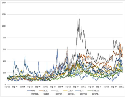
Table 1. Descriptive statistics.

		LEVEL		RETURNS
		MEAN	STD.DEV.	MEAN	STD.DEV.	MIN.	MAX.	SKEWNESS	KURTOSIS
Panel A: Futures Prices
GAS	USD	3.99	2.21	0.042	7.47	−37.17	48.25	0.13	5.69
HOIL	USD	1.57	0.94	0.105	5.02	−38.16	35.10	0.00	9.33
OIL	USD	51.98	29.48	0.081	5.73	−69.76	68.83	−0.36	31.20
CORN	USc	365.91	156.63	0.073	3.90	−32.78	23.25	−0.61	9.80
SOY	USc	888.45	331.18	0.064	3.41	−22.84	12.03	−0.80	7.51
WHEAT	USc	484.34	185.05	0.053	4.22	−23.37	23.96	0.26	5.20
COPPER	USD	2.20	1.20	0.082	3.34	−18.28	18.08	−0.25	5.08
GOLD	USD	878.37	544.95	0.105	2.22	−13.43	16.86	0.10	8.01
SILVER	USD	13.31	8.74	0.117	4.03	−30.44	22.64	−0.52	7.95
COCOA	USc	1982.52	712.34	0.062	4.14	−17.21	23.77	0.25	5.21
COFFEE	USc	127.00	49.36	0.068	5.17	−31.29	28.46	0.33	5.69
SUGAR	USD	13.28	5.43	0.031	4.53	−22.98	17.13	−0.13	4.49
	OVERALL				52-WK HIGH		52-WK LOW
	MEAN	STD.DEV.	MIN	MAX	MEAN	Diff.	MEAN	Diff.
Panel B: Net Commercial Positions
GAS	0.004	0.108	−0.31	0.24	−0.042	***	0.087	***
HOIL	−0.087	0.085	−0.33	0.13	−0.160	***	0.011	***
OIL	−0.088	0.107	−0.30	0.23	−0.129	***	−0.046	***
CORN	−0.035	0.134	−0.31	0.34	−0.185	***	0.130	***
SOY	−0.097	0.161	−0.46	0.33	−0.232	***	0.095	***
WHEAT	−0.007	0.139	−0.43	0.25	−0.112	***	0.086	***
COPPER	−0.068	0.200	−0.56	0.36	−0.267	***	0.136	***
GOLD	−0.263	0.260	−0.64	0.47	−0.486	***	0.116	***
SILVER	−0.373	0.167	−0.75	0.07	−0.491	***	−0.140	***
COCOA	−0.128	0.155	−0.54	0.37	−0.244	***	0.040	***
COFFEE	−0.118	0.160	−0.54	0.26	−0.296	***	0.067	***
SUGAR	−0.151	0.176	−0.61	0.38	−0.332	***	0.052	***
	OVERALL				52-WK HIGH		52-WK LOW
	MEAN	STD.DEV.	MIN	MAX	MEAN	Diff.	MEAN	Diff.
Panel C: Net Noncommercial Positions
GAS	−0.053	0.095	−0.27	0.18	−0.006	***	−0.127	***
HOIL	0.031	0.061	−0.16	0.21	0.087	***	−0.037	***
OIL	0.085	0.095	−0.17	0.29	0.119	***	0.054	***
CORN	0.095	0.122	−0.21	0.35	0.233	***	−0.044	***
COCOA	0.085	0.144	−0.36	0.41	0.195	***	−0.067	***
SOY	0.109	0.136	−0.30	0.35	0.240	***	−0.057	***
WHEAT	0.004	0.119	−0.29	0.38	0.124	***	−0.101	***
COPPER	0.032	0.155	−0.32	0.44	0.208	***	−0.148	***
GOLD	0.194	0.233	−0.45	0.53	0.386	***	−0.120	***
SILVER	0.226	0.137	−0.14	0.58	0.342	***	0.037	***
COFFEE	0.063	0.151	−0.30	0.40	0.246	***	−0.116	***
SUGAR	0.101	0.140	−0.27	0.43	0.239	***	−0.054	***

Note: This table provide descriptive statistics for the futures market variables used in this study. Variables include returns for the natural gas, heating oil, crude oil, corn, soymeal, wheat, copper, gold, silver, cocoa, coffee, and sugar futures markets. Panel A reports statistics for futures prices, including weekly log returns. Panel B reports statistics for positions held by commercial traders and Panel C reports statistics for noncommercial traders. CFTC COT reports are used to compute net positions of different trader types (scaled by open interest). First differences are reported for net positions since they take both negative and positive values. Statistics are reported for the overall sample period and when the market has reached a 52-week high or low in the prior week. Differences from the overall sample are indicated together with level of significance as determined by t-tests (*** indicating significance at 1% level). Sample Period: September 1992–December 2022.

Table 1 provides descriptive statistics for the futures contracts used in our study. Panel A shows the return for each futures contract. All commodities exhibit a positive weekly return on average during our sample period, this ranges from 0.042 (natural gas) to 0.117 (silver). Natural gas generates the most volatile returns (7.47) and gold the least volatile (2.22). In addition, kurtosis indicates that all commodities exhibit ‘fat-tails’ in the return distribution that is common among financial assets.

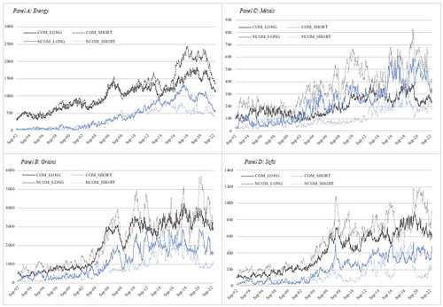
We obtain trader position information from the CFTC’s weekly COT report⁷ which requires all reportable traders to report their open futures positions as of Tuesday of the given week. We utilize the ‘legacy report’ classifications that classify traders as commercial (COM) – this includes producers, merchants, processors, and users of the commodity – or noncommercial (NCOM).⁸ We do not include the traders with small ‘non-reportable’ positions in our analysis. This report provides the long, short, and spread positions for each trader type. In Figure 2, we aggregate the positions⁹ for each of our classifications (energy, grains, metals, softs) to illustrate how the long and short positions have evolved during our sample period. We note that position sizes have increased over time and that there was a sharp increase across all commodities just prior to the GFC. Aside from metals, commercial traders account for the greatest increases in position size.

Figure 2. Outright positions by trader type.

Note: This figure illustrates the outright long and short positions for commercial (COM) and non-commercial (NCOM) traders. Panel A averages the positions for energy futures (GAS, HOIL, OIL), Panel B for grain futures (CORN, SOY, WHEAT), Panel C for metal futures (COPPER, GOLD, SILVER), and Panel D for softs futures (COCOA, COFFEE, SUGAR). NB: Energy futures are scaled by 103 to ease readability.

We focus our analysis on the net position (NP_jkt) in commodity j of each trader type k during week t. This is computed using the long and short positions for each trader type and then scaled by open interest (OI_jt) to control for the variation in market size over time¹⁰ (indicated in Figure 2). (1) $${\mathit{\text{NP}}}_{\mathit{\text{jkt}}}=\frac{{\mathit{\text{Long}}}_{\mathit{\text{jkt}}}-{\mathit{\text{Short}}}_{\mathit{\text{jkt}}}}{{\mathit{\text{OI}}}_{\mathit{\text{jt}}}}\mathrm{ }$$(1)

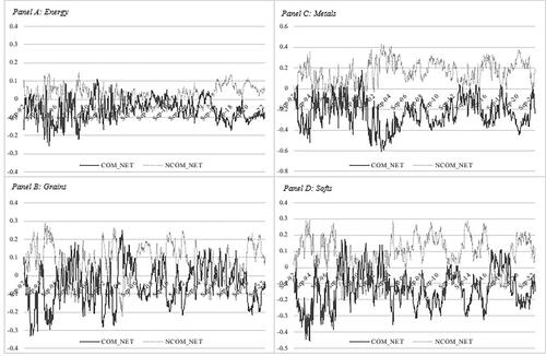
Panel B of Table 1 shows that commercial positions tend to be net short on average (natural gas is the only exception) and noncommercial traders are net long.¹¹ Figure 3 illustrates how positions vary over time. The data is consistent with commercial traders using futures to hedge a long position in the underlying commodity from the production process (short hedgers) outnumbering consumers of the commodity who would hedge a short position in the underlying by buying futures (long hedgers). Similarly, the figure is consistent with noncommercial traders tending to be speculate on increases in commodity prices. The largest net positions are in gold and silver, and they also offer the most extreme positioning. This panel also provides a first indication as to how trading positions vary around the 52-week high and low prices. At the 52-week high, commercial (noncommercial) positions are shorter (longer) than in the overall sample. In contrast, at the 52-week low, commercial positions are long (or less short in the case of crude oil and silver) while noncommercial positions are short (or less long for crude oil and silver). The significance of these observations is confirmed as better than 1% according to t-tests and Welch F-tests. Together, the observations indicate that commercial traders follow a contrarian strategy (shorting when the market is high and buying when the market is low) while noncommercial traders follow a momentum strategy (buying when the market is high and selling when the market is low).

Figure 3. Net positions by trader type.

Note: This figure illustrates the net positions for commercial (COM) and non-commercial (NCOM) traders. Panel A averages the positions for energy futures (GAS, HOIL, OIL), Panel B for grain futures (CORN, SOY, WHEAT), Panel C for metal futures (COPPER, GOLD, SILVER), and Panel D for softs futures (COCOA, COFFEE, SUGAR).

Methodology

To examine the effect of 52-week highs and lows on trading behavior, we augment the models used in Wang (2003) and Baur and Smales (2022) by incorporating variables to indicate whether the market is trading at a 52-week high (HI52) or low (LO52). Our baseline model is shown in Equation (2)(2) $${\Delta \mathit{\text{NP}}}_{\mathit{\text{jkt}}}={\alpha }_0+{\alpha }_1{R}_{t-1}+{\alpha }_2{\mathit{\text{HI}}52}_{t-1}+{\alpha }_3{H{I52}_{t-1}\times R}_{t-1}+{\alpha }_4{\mathit{\text{LO}}52}_{t-1}+{\alpha }_5{\mathit{\text{LO}}{52}_{t-1}\times R}_{t-1}+{\alpha }_6{\Delta \mathit{\text{NP}}}_{\mathit{\text{jkt}}-1}+\sum {\beta }_m{\mathrm{\Phi }}_{t-1}+{\epsilon }_t\mathrm{ }$$(2) : (2) $${\Delta \mathit{\text{NP}}}_{\mathit{\text{jkt}}}={\alpha }_0+{\alpha }_1{R}_{t-1}+{\alpha }_2{\mathit{\text{HI}}52}_{t-1}+{\alpha }_3{H{I52}_{t-1}\times R}_{t-1}+{\alpha }_4{\mathit{\text{LO}}52}_{t-1}+{\alpha }_5{\mathit{\text{LO}}{52}_{t-1}\times R}_{t-1}+{\alpha }_6{\Delta \mathit{\text{NP}}}_{\mathit{\text{jkt}}-1}+\sum {\beta }_m{\mathrm{\Phi }}_{t-1}+{\epsilon }_t\mathrm{ }$$(2) where ΔNP_jkt is the change in net position of futures market j for trader type k in week t, and R_t-1 is the applicable futures return in the prior week. We include dummy variables to indicate market is trading at the 52-week high (HI52) or low (LO52) and interact with weekly market returns. ΔNP_jkt-1 is included to account for serial correlation.¹² Φ is a set of control variables. This includes the 3-month T-Bill yield (TBILL), the difference between the yield on Baa-rated and Aaa-rated corporate bonds (CRDSPRD), and the S&P500 index dividend yield (DIVYLD) that Bessembinder and Chan (1992) show are priced factors in future markets. We further control for US financial market uncertainty, proxied by the CBOE volatility index (VIX), and the term structure of interest rates, defined as the difference between 2-year and 10-year government bond yields (TERM). Finally, to control for the potential of different trading preferences when the market is in backwardation, i.e., the spot price is higher than the futures price, we add an indicator variable (BACK). ε is the Newey-West standard error that is robust to heteroskedasticity.

For the empirical results to be consistent with our initial observation that commercial traders are following a contrarian strategy, the estimated coefficients for α₁ and α₂ should be negative (positions are shorter, or less long, when returns are positive or when prices reach a 52-week high) and α₄ should be positive (positions are longer, or less short, when prices reach a 52-week low). Conversely, to demonstrate that noncommercial traders are following a momentum strategy we would find that α₁ and α₂ should be positive and α₄ negative.

Empirical results

Trading behavior at the 52-week high and low

We report the results of our baseline regression model for commercial traders in Table 2, and for noncommercial traders in Table 3. The results largely confirm our expectations as to the strategies adopted by different types of traders. First, the estimated coefficient for lagged returns is negative for commercial traders and positive for noncommercial traders. This shows that, in general, commercial traders become shorter (less long) following positive returns while noncommercial traders become longer (less short). Second, the estimated coefficients for the 52-week high is also negative for commercial traders and positive for noncommercial traders. This demonstrates that commercial traders become shorter at the 52-week high while noncommercial traders become longer. Third, the estimated coefficients for the 52-week low are positive (negative) for commercial (noncommercial) traders. The results are consistent across all futures markets – and only the only statistically insignificant estimates are LO52 for the natural gas (GAS) and heating oil (HOIL) markets. In other words, we have support for our ex-ante expectation that commercial traders follow contrarian strategies while noncommercial traders follow momentum strategies. This result is also consistent with the likes of Sanders, Boris, and Manfredo (2004), Sanders, Irwin, and Merrin (2009) and Kang, Rouwenhorst, and Tang (2020). One explanation is that commercial traders are anchored to recent prices while noncommercial traders trade attention-grabbing commodities.

Table 2. Regression: influence of 52-week highs and lows on trading behavior of commercial traders.

	ENERGY			GRAINS			METALS			SOFTS
DEP: ΔNPt	GAS	HOIL	OIL	CORN	SOY	WHEAT	COPPER	GOLD	SILVER	COCOA	COFFEE	SUGAR
Intercept	0.025	0.058	0.062	0.373**	0.227	0.610***	0.113	−1.518***	−1.108	−0.190	−0.202	−0.101
	(0.126)	(0.118)	(0.104)	(0.162)	(0.140)	(0.212)	(0.187)	(0.403)	(1.032)	(0.146)	(0.381)	(0.210)
Rt-1	−0.041***	−0.081***	−0.057***	−0.093***	−0.046*	−0.133***	−0.246***	−0.208***	−0.163***	−0.181***	−0.163***	−0.075*
	(0.008)	(0.020)	(0.017)	(0.024)	(0.028)	(0.026)	(0.047)	(0.059)	(0.036)	(0.027)	(0.030)	(0.041)
HI52	−0.488**	−1.153***	−0.477***	−1.035***	−1.329***	−2.243***	−1.701***	−1.089***	−1.300***	−1.187***	−1.348***	−1.585***
	(0.229)	(0.268)	(0.165)	(0.226)	(0.193)	(0.436)	(0.375)	(0.403)	(0.423)	(0.341)	(0.417)	(0.511)
HI52·Rt-1	0.034*	0.165***	0.027	0.051	0.107*	0.129***	0.371***	0.595***	0.421***	0.187***	0.187***	0.256***
	(0.021)	(0.054)	(0.040)	(0.063)	(0.061)	(0.050)	(0.100)	(0.128)	(0.086)	(0.063)	(0.068)	(0.090)
LO52	0.206	0.503*	0.719**	1.867***	0.898***	1.390***	1.727***	3.139***	3.335***	1.791***	3.081***	1.828***
	(0.213)	(0.275)	(0.346)	(0.383)	(0.387)	(0.412)	(0.511)	(0.693)	(0.460)	(0.486)	(0.377)	(0.484)
LO52·Rt-1	0.056*	0.107**	0.135***	0.156***	0.065	0.219***	0.498***	0.272	0.376***	0.043	0.216**	−0.200
	(0.031)	(0.045)	(0.032)	(0.051)	(0.080)	(0.081)	(0.112)	(0.291)	(0.135)	(0.114)	(0.090)	(0.171)
ΔNPt-1	0.144***	0.095***	0.069*	0.183***	0.196***	0.078**	0.182***	0.126***	0.136***	0.133***	0.144***	0.222***
	(0.031)	(0.031)	(0.041)	(0.030)	(0.037)	(0.036)	(0.034)	(0.036)	(0.036)	(0.029)	(0.041)	(0.032)
ΔVIXt-1	0.018	0.016	0.007	−0.022	0.006	0.028	−0.001	0.016	−0.021	0.077*	−0.008	−0.131**
	(0.032)	(0.037)	(0.031)	(0.030)	(0.036)	(0.045)	(0.053)	(0.063)	(0.060)	(0.042)	(0.057)	(0.062)
ΔTBILLt-1	−0.221	−1.849**	−1.028	−1.416*	0.476	−1.225	0.540	3.577*	0.530	−0.571	−1.189	−1.628
	(0.558)	(0.728)	(0.843)	(0.815)	(1.018)	(1.188)	(1.182)	(2.096)	1.498	(0.794)	(1.201)	(1.414)
ΔCRDSPRDt-1	0.019	−0.481	−0.079	−0.474	−0.914	−0.312	4.040	2.855	1.337	2.682**	2.812	−1.591
	(0.637)	(1.445)	(1.086)	(1.018)	(1.515)	(1.891)	(2.454)	(2.853)	(2.234)	(1.364)	(1.836)	(1.772)
ΔTERMt-1	0.254	−1.958*	−0.749	−1.021	0.231	−0.947	−1.548	3.868*	−1.630	−2.020*	−2.011	−1.507
	(0.670)	(1.014)	(0.921)	(1.086)	(0.969)	(1.302)	(1.452)	(2.062)	(1.489)	(1.039)	(1.341)	(1.359)
ΔDIVYLDt-1	0.257	5.726***	3.210**	4.228**	5.138**	4.399	14.740***	1.325	2.723	1.657	4.455	5.999*
	(1.519)	(2.132)	(1.622)	(1.784)	(2.270)	(2.760)	(4.122)	(3.715)	(3.616)	(2.309)	(3.245)	(3.338)
BACKt-1	0.017	0.028	−0.074	−0.449**	−0.247	−0.599**	−0.042	1.431***	0.973	0.279	0.073	−0.051
	(0.140)	(0.147)	(0.128)	(0.178)	(0.169)	(0.235)	(0.237)	(0.423)	(1.047)	(0.182)	(0.387)	(0.268)
Adj. R^2	0.047	0.051	0.036	0.107	0.075	0.065	0.113	0.048	0.081	0.118	0.107	0.109
F-Statistic	7.22	7.88	5.76	16.23	11.39	9.80	17.20	7.45	12.20	18.07	16.30	16.64
Durbin-Watson	1.98	1.99	2.01	1.92	1.97	1.95	1.93	1.95	1.95	1.98	1.93	1.94
No. Obs.	1528	1528	1528	1528	1528	1528	1528	1528	1528	1528	1528	1528

Note: This table reports the estimated coefficients for the model specified in Equation (2). The dependent variable is the weekly change in net position (NP) for commercial traders. The key explanatory variables are lagged log returns (R), a dummy variable indicating the market is trading at a 52-week high (HI52), or low (LO52), and associated interaction terms (HI52·R; LO52·R). Control variables include the lagged dependent variables, lagged changes in S&P500 implied volatility index (VIX), 3-month US T-Bill rate (TBILL), Baa-Aaa credit spread (CRDSPRD), the 10-yr minus 2-yr US government bond yield spread (TERM), the S&P500 dividend yield (DIVYLD), and a dummy variable signifying whether the futures market is in backwardation (BACK). Newey-West standard errors are reported in parentheses. *, **, *** indicates statistical significance at the 10%, 5%, and 1% level respectively. Sample Period: September 1992–December 2022.

Table 3. Regression: influence of 52-week highs and lows on trading behavior of noncommercial traders.

	ENERGY			GRAINS			METALS			SOFTS
DEP: ΔNPt	GAS	HOIL	OIL	CORN	SOY	WHEAT	COPPER	GOLD	SILVER	COCOA	COFFEE	SUGAR
Intercept	−0.038	−0.060	−0.080	−0.255*	−0.170	−0.531***	−0.091	1.347***	0.391	0.176	0.158	0.098
	(0.101)	(0.089)	(0.080)	(0.144)	(0.121)	(0.203)	(0.146)	(0.351)	(1.089)	(0.130)	(0.333)	(0.150)
Rt-1	0.035***	0.073***	0.034***	0.110***	0.077***	0.123***	0.197***	0.199***	0.157***	0.189***	0.166***	0.075**
	(0.007)	(0.016)	(0.013)	(0.023)	(0.026)	(0.023)	(0.038)	(0.049)	(0.028)	(0.023)	(0.029)	(0.037)
HI52	0.590***	0.847***	0.589***	0.864***	1.014***	1.875***	1.419***	0.870**	1.276***	0.828**	1.370***	0.887**
	(0.210)	(0.232)	(0.147)	(0.202)	(0.188)	(0.429)	0.307	(0.352)	(0.470)	(0.337)	(0.373)	(0.390)
HI52·Rt-1	−0.054***	−0.124***	−0.039	−0.064	−0.078	−0.163***	−0.281***	−0.470***	−0.419***	−0.130**	−0.176***	−0.154**
	(0.019)	(0.046)	(0.032)	(0.063)	(0.061)	(0.051)	(0.084)	(0.103)	(0.094)	(0.065)	(0.065)	(0.078)
LO52	−0.131	−0.323	−0.604**	−1.562***	−0.944***	−0.837**	−1.159***	−2.435***	−2.421***	−1.527***	−2.908***	−1.236***
	(0.207)	(0.239)	(0.239)	(0.330)	(0.356)	(0.347)	(0.382)	(0.555)	(0.393)	(0.438)	(0.382)	(0.350)
LO52·Rt-1	−0.037	−0.099***	−0.123***	−0.133**	−0.092	−0.103	−0.312***	−0.193	−0.295**	−0.056	−0.230***	0.160
	(0.029)	(0.037)	(0.026)	(0.054)	(0.075)	(0.091)	(0.084)	(0.236)	(0.119)	(0.107)	(0.083)	(0.137)
ΔNPt-1	0.153***	0.044	0.088**	0.198***	0.171***	0.089**	0.195***	0.133***	0.175***	0.137***	0.161***	0.243***
	(0.031)	(0.033)	(0.036)	(0.028)	(0.037)	(0.036)	(0.032)	(0.034)	(0.031)	(0.027)	(0.041)	(0.034)
ΔVIXt-1	−0.017	−0.007	0.004	0.029	0.007	−0.022	−0.002	−0.012	0.021	−0.086**	0.011	0.097**
	(0.029)	(0.028)	(0.024)	(0.030)	(0.033)	(0.042)	(0.043)	(0.051)	(0.053)	(0.039)	(0.052)	(0.043)
ΔTBILLt-1	−0.089	0.837	0.924	1.196*	0.049	1.083	−0.531	−2.990*	−0.712	−0.018	0.873	1.494
	(0.472)	(0.518)	(0.632)	(0.717)	(0.878)	(1.026)	(0.988)	(1.709)	(1.401)	(0.739)	(1.139)	(0.969)
ΔCRDSPRDt-1	0.327	0.248	−0.472	0.912	0.296	0.492	−3.002	−1.503	−2.845	−2.745**	−2.255	1.284
	(0.623)	(1.056)	(0.987)	(1.018)	(1.550)	(1.777)	(2.062)	(2.238)	(2.120)	(1.234)	(1.729)	(1.242)
ΔTERMt-1	−0.315	1.165	0.871	0.633	0.503	0.346	1.483	−3.797*	2.058	1.496*	1.664	0.783
	(0.562)	(0.753)	(0.739)	(1.060)	(0.947)	(1.184)	(1.181)	(1.679)	(1.562)	(0.880)	(1.217)	(0.996)
ΔDIVYLDt-1	0.141	−4.592***	−3.998***	−3.758**	−4.381**	−4.066	−9.919***	2.090	−0.906	−0.111	−3.700	−4.007*
	(0.155)	(1.535)	(1.287)	(1.654)	(2.115)	(2.550)	(3.048)	(3.047)	(3.298)	(2.100)	(2.922)	(2.325)
BACKt-1	−0.003	−0.004	0.081	0.317*	0.210	0.535**	0.021	−1.284***	−0.291	−0.244	−0.036	0.015
	(0.113)	(0.109)	0.099	(0.163)	(0.154)	(0.223)	(0.189)	(0.366)	(1.097)	(0.162)	(0.342)	(0.196)
Adj. R^2	0.051	0.043	0.045	0.115	0.068	0.061	0.113	0.053	0.092	0.132	0.124	0.131
F-Statistic	7.75	6.76	6.94	17.61	10.22	9.22	17.34	8.15	13.87	20.29	19.03	20.14
Durbin-Watson	1.97	1.99	1.99	1.93	1.97	1.96	1.93	1.95	1.94	1.99	1.93	1.95
No. Obs.	1528	1528	1528	1528	1528	1528	1528	1528	1528	1528	1528	1528

Note: This table reports the estimated coefficients for the model specified in Equation (2). The dependent variable is the weekly change in net position (NP) for noncommercial traders. The key explanatory variables are lagged log returns (R), a dummy variable indicating the market is trading at a 52-week high (HI52), or low (LO52), and associated interaction terms (HI52·R; LO52·R). Control variables include the lagged dependent variables, lagged changes in S&P500 implied volatility index (VIX), 3-month US T-Bill rate (TBILL), Baa-Aaa credit spread (CRDSPRD), the 10-yr minus 2-yr US government bond yield spread (TERM), the S&P500 dividend yield (DIVYLD), and a dummy variable signifying whether the futures market is in backwardation (BACK). Newey-West standard errors are reported in parentheses. *, **, *** indicates statistical significance at the 10%, 5%, and 1% level respectively. Sample Period: September 1992–December 2022.

We now turn to the 52-week interaction terms. The positive (negative) HI52·R interaction terms found for commercial (noncommercial) suggest that both trader types moderate their strategy at the 52-week high. This is consistent with the anchor revision noted by Blau et al. (2023) in stock markets. An explanation specific to commodity markets could be that commercial producers are already benefiting from selling the underlying commodity at high prices and so are less response to further positive gains. Noncommercial speculators, who tend to be long, have already benefited from rising prices in futures markets and so are also less responsive to further gains. Conversely, the direction of the LO52·R interaction terms indicate that both trader types accentuate their trading strategy at the 52-week low. It is possible that producers are receiving low prices for the underlying commodity and are less willing to lock in those prices, thus reducing their net short (or going long) in the hope of future price rises. In sum, the estimates suggest that trading behavior is moderated at the 52-week high and accentuated at the 52-week low, for both trader types.

Finally, the majority of estimated coefficients for the control variables are insignificant. However, we note that, when the respective market is in backwardation, commercial traders buy gold futures and sell grain futures, while noncommercial traders do the opposite. When the dividend yield increases, which is commonly associated with stock market declines, commercial traders buy futures and noncommercial traders sell futures.

We use pairwise Granger Causality tests to provide additional evidence as to the relationship between returns and changes in net positions. The results reported in Table 4 demonstrate that the relationship tends to be unidirectional with returns causing changes in net positions for both commercial (Panel A) and noncommercial (Panel B) traders. The limited exceptions are the bidirectional relationships for cocoa (commercial only) and sugar (commercial and noncommercial), and the causality running from position changes to returns for soy (commercial). Together, the results suggest that both trader types adjust their positions in response to market returns rather than vice-versa.

Table 4. Granger causality tests.

Panel A: Commercial					Panel B: Noncommercial
Null Hypothesis:	Obs.	F-Statistic	Prob.		Null Hypothesis:	Obs.	F-Statistic	Prob.
RGAS does not Granger Cause ΔNPGAS	1572	7.552	<0.001		RGAS does not Granger Cause ΔNPGAS	1572	6.610	<0.001
ΔNPGAS does not Granger Cause RGAS		1.321	0.252		ΔNPGAS does not Granger Cause RGAS		0.749	0.587
RHOIL does not Granger Cause ΔNPHOIL	1572	5.482	<0.001		RHOIL does not Granger Cause ΔNPHOIL	1572	7.205	<0.001
ΔNPHOIL does not Granger Cause RHOIL		0.435	0.824		ΔNPHOIL does not Granger Cause RHOIL		0.708	0.617
ROIL does not Granger Cause ΔNPOIL	1572	7.882	<0.001		ROIL does not Granger Cause ΔNPOIL	1572	5.984	<0.001
ΔNPOIL does not Granger Cause ROIL		1.256	0.280		ΔNPOIL does not Granger Cause ROIL		0.777	0.566
RCORN does not Granger Cause ΔNPCORN	1572	3.319	<0.001		RCORN does not Granger Cause ΔNPCORN	1572	5.522	<0.001
ΔNPCORN does not Granger Cause RCORN		0.416	0.838		ΔNPCORN does not Granger Cause RCORN		0.248	0.941
RSOY does not Granger Cause ΔNPSOY	1572	1.767	0.117		RSOY does not Granger Cause ΔNPSOY	1572	3.084	0.009
ΔNPSOY does not Granger Cause RSOY		3.129	0.008		ΔNPSOY does not Granger Cause RSOY		2.421	0.034
RWHEAT does not Granger Cause ΔNPWHEAT	1572	4.207	0.001		RWHEAT does not Granger Cause ΔNPWHEAT	1572	5.743	<0.001
ΔNPWHEAT does not Granger Cause RWHEAT		0.814	0.539		ΔNPWHEAT does not Granger Cause RWHEAT		0.427	0.830
RCOPPER does not Granger Cause ΔNPCOPPER	1572	6.436	<0.001		RCOPPER does not Granger Cause ΔNPCOPPER	1572	6.466	<0.001
ΔNPCOPPER does not Granger Cause RCOPPER		1.123	0.346		ΔNPCOPPER does not Granger Cause RCOPPER		0.961	0.440
RGOLD does not Granger Cause ΔNPGOLD	1572	1.517	0.181		RGOLD does not Granger Cause ΔNPGOLD	1572	1.846	0.101
ΔNPGOLD does not Granger Cause RGOLD		0.701	0.623		ΔNPGOLD does not Granger Cause RGOLD		0.550	0.738
RSILVER does not Granger Cause ΔNPSILVER	1572	4.242	0.001		RSILVER does not Granger Cause ΔNPSILVER	1572	4.034	0.001
ΔNPSILVER does not Granger Cause RSILVER		0.820	0.535		ΔNPSILVER does not Granger Cause RSILVER		0.380	0.863
RCOCOA does not Granger Cause ΔNPCOCOA	1572	11.030	<0.001		RCOCOA does not Granger Cause ΔNPCOCOA	1572	15.477	<0.001
ΔNPCOCOA does not Granger Cause RCOCOA		3.291	0.006		ΔNPCOCOA does not Granger Cause RCOCOA		2.099	0.063
RCOFFEE does not Granger Cause ΔNPCOFFEE	1572	5.215	<0.001		RCOFFEE does not Granger Cause ΔNPCOFFEE	1572	7.215	<0.001
ΔNPCOFFEE does not Granger Cause RCOFFEE		1.794	0.111		ΔNPCOFFEE does not Granger Cause RCOFFEE		2.226	0.049
RSUGAR does not Granger Cause ΔNPSUGAR	1572	4.315	0.001		RSUGAR does not Granger Cause ΔNPSUGAR	1572	7.016	<0.001
ΔNPSUGAR does not Granger Cause RSUGAR		6.982	<0.001		ΔNPSUGAR does not Granger Cause RSUGAR		6.071	<0.001

Note: This table shows results of pairwise Granger causality tests for returns (R) and changes in net positions (ΔNP) of commercial (Panel A) and noncommercial (Panel B) traders in a range of futures markets. Four lags are used on the basis of optimal AIC and SIC. Sample period: September 1992–December 2022.

There is evidence that commodities tend to perform better when the market is in backwardation rather than contango (e.g., Levine et al. 2018) and that traders seem to adjust their positions in response to this (e.g., Alizadeh and Tamvakis 2016). Given this information, we disaggregate our sample according to the market condition and repeat our earlier analysis in Table 5.¹³ We find that the response to returns is consistent across market conditions. That is, commercial traders tend to be contrarian while noncommercial traders follow a momentum strategy regardless of whether the market is in backwardation or contango. We note similarities in our results across trader-types, indicating that market condition has a similar influence on both commercial and noncommercial traders. The general finding is that 52-week high prices have a significant influence on trader positions regardless of market state, but 52-week low prices only have a significant influence when the market is in backwardation. Backwardation typically occurs due to supply shortages (or demand spikes) in the physical commodity and results in futures pricing falling below those of the physical. It is possible that a 52-week low futures price that is below the current physical price offers a compelling reason for hedgers to attenuate (reduce) their hedge.

Table 5. Importance of market condition (Backwardation & Contango).

	GAS		HOIL		OIL		CORN		SOY		WHEAT		COPPER		COCOA		COFFEE		SUGAR
	BACK	CONT	BACK	CONT	BACK	CONT	BACK	CONT	BACK	CONT	BACK	CONT	BACK	CONT	BACK	CONT	BACK	CONT	BACK	CONT
Panel A: Commercial Traders
Intercept	0.036	0.051	0.111	0.011	0.010	0.046	−0.060	0.288	0.005	0.179	0.056	0.512*	0.101	0.032	0.107	−0.232	−0.069	−0.488	−0.147	−0.129
	(0.067)	(0.133)	(0.105)	(0.131)	(0.079)	(0.115)	(0.091)	(0.178)	(0.119)	(0.143)	(0.105)	(0.262)	(0.180)	(0.207)	(0.113)	(0.150)	(0.128)	(0.504)	(0.164)	(0.225)
Rt-1	−0.048***	−0.029**	−0.075***	−0.087***	−0.041**	−0.091***	−0.089***	−0.104**	−0.095**	−0.019	−0.115***	−0.173***	−0.312***	−0.161**	−0.213***	−0.098***	−0.169***	−0.175**	−0.048	−0.182***
	(0.009)	(0.012)	(0.027)	(0.029)	(0.017)	(0.024)	(0.027)	(0.043)	(0.044)	(0.039)	(0.028)	(0.065)	(0.064)	(0.066)	(0.036)	(0.037)	(0.035)	(0.068)	(0.032)	(0.049)
HI52	−0.461	−0.565	−1.593***	−0.715**	−0.914***	−0.252	−1.189***	−0.762***	−1.403***	−1.329***	−2.845***	−1.509**	−1.981***	−1.167**	−1.389***	−0.886*	−1.802***	0.645	−0.778	−1.958***
	(0.286)	(0.399)	(0.415)	(0.306)	(0.276)	(0.201)	(0.308)	(0.286)	(0.278)	(0.289)	(0.566)	(0.617)	(0.535)	(0.458)	(0.477)	(0.486)	(0.370)	(1.335)	(0.561)	(0.635)
HI52·Rt-1	0.055*	0.015	0.163*	0.155**	0.046	0.033	0.010	0.139**	0.107	0.136	0.125*	0.163	0.374**	3.140***	0.220***	0.117	0.186***	0.122	0.107	0.398***
	(0.030)	(0.028)	(0.094)	(0.061)	(0.051)	(0.054)	(0.085)	(0.066)	(0.082)	(0.090)	(0.066)	(0.103)	(0.148)	(0.120)	(0.079)	(0.095)	(0.047)	(0.169)	(0.080)	(0.118)
LO52	0.241	−0.461	0.557*	0.392	0.742*	0.194	1.977***	0.956	0.761*	1.218	1.121***	5.205**	1.617***	1.591	1.649***	3.209*	2.840***	4.988***	1.593***	3.250
	(0.218)	(0.880)	(0.325)	(0.404)	(0.383)	(0.386)	(0.406)	(1.073)	(0.427)	(0.776)	(0.389)	(2.497)	(0.593)	(1.076)	(0.512)	(1.698)	(0.381)	(1.540)	(0.476)	(2.123)
LO52·Rt-1	0.065***	−0.040	0.009*	0.204**	0.123***	−0.096	0.189***	0.096	0.162**	−0.063	0.186**	0.885	0.443***	0.460***	0.074	0.062	0.249**	0.299*	−0.200	−0.246
	(0.032)	(0.077)	(0.051)	(0.101)	(0.033)	(0.089)	(0.068)	(0.064)	(0.079)	(0.173)	(0.076)	(0.709)	(0.141)	(0.155)	(0.119)	(0.398)	(0.104)	(0.167)	(0.173)	(0.540)
CONTROLS	YES	YES	YES	YES	YES	YES	YES	YES	YES	YES	YES	YES	YES	YES	YES	YES	YES	YES	YES	YES
Adj. R^2	0.044	0.038	0.055	0.037	0.056	0.026	0.105	0.093	0.061	0.091	0.076	0.036	0.127	0.086	0.105	0.148	0.114	0.079	0.140	0.090
No. Obs.	1214	314	995	533	826	702	1223	305	902	626	1254	274	966	562	1091	437	1287	241	830	698
	GAS		HOIL		OIL		CORN		SOY		WHEAT		COPPER		COCOA		COFFEE		SUGAR
	BACK	CONT	BACK	CONT	BACK	CONT	BACK	CONT	BACK	CONT	BACK	CONT	BACK	CONT	BACK	CONT	BACK	CONT	BACK	CONT
Panel B: Noncommercial Traders
Intercept	−0.031	−0.071	−0.081	−0.023	−0.016	−0.066	0.037	−0.153	0.014	−0.135	−0.030	−0.401*	−0.096	−0.014	−0.085	0.228*	0.079	0.312	0.096	0.130
	(0.057)	(0.108)	(0.079)	(0.094)	(0.062)	(0.088)	(0.088)	(0.156)	(0.118)	(0.129)	(0.098)	(0.238)	(0.147)	(0.161)	(0.100)	(0.133)	(0.121)	(0.435)	(0.122)	(0.156)
Rt-1	0.043***	0.021**	0.074***	0.071***	0.025*	0.053***	0.114***	0.095**	0.158***	0.032	0.124***	0.119**	0.261***	0.117**	0.217***	0.121***	0.178***	0.149**	0.054*	0.158***
	(0.008)	(0.010)	(0.019)	(0.024)	(0.013)	(0.019)	(0.026)	(0.041)	(0.043)	(0.032)	(0.025)	(0.058)	(0.051)	(0.055)	(0.031)	(0.032)	(0.033)	(0.071)	(0.032)	(0.034)
HI52	0.430	0.826**	1.029***	0.658**	0.817***	0.464***	1.027***	0.587**	1.138***	0.956***	2.565***	0.981*	1.704***	0.882**	0.977**	0.540	1.743***	−0.179	0.396	1.131**
	(0.271)	(0.342)	(0.346)	(0.289)	(0.268)	(0.177)	(0.286)	(0.230)	(0.279)	(0.255)	(0.588)	(0.580)	(0.416)	(0.442)	(0.487)	(0.448)	(0.351)	(1.246)	(0.504)	(0.480)
HI52·Rt-1	−0.055*	−0.047*	−0.078	−0.153***	−0.024	−0.052	−0.007	−0.179***	−0.121	−0.074	−0.190***	−0.131	−0.294**	−0.217**	−0.132	−0.094	−0.164***	−0.106	0.004	−0.290***
	(0.032)	(0.024)	(0.084)	(0.053)	(0.055)	(0.041)	(0.087)	(0.050)	(0.088)	(0.081)	(0.069)	(0.099)	(0.115)	(0.107)	(0.087)	(0.094)	(0.047)	(0.157)	(0.079)	(0.096)
LO52	−0.168	0.602	−0.343	−0.334	−0.598**	−0.320	−1.702***	−0.962	−0.795*	−1.235*	−0.716**	−2.921	−1.165**	−0.754	−1.441***	−2.555**	−2.788***	−3.776**	−1.045***	−2.248
	(0.210)	(0.727)	(0.280)	(0.269)	(0.263)	(0.357)	(0.332)	(1.106)	(0.410)	(0.664)	(0.348)	(1.827)	(0.460)	(0.680)	(0.471)	(1.282)	(0.391)	(1.598)	(0.329)	(1.586)
LO52·Rt-1	−0.048	0.074	−0.090**	−0.177***	−0.119***	0.033	−0.208***	−0.019	−0.198**	0.011	−0.086	−0.616	−0.309***	−0.201	−0.087	−0.046	−0.240**	−0.305	0.164	0.220
	(0.030)	(0.061)	(0.041)	(0.061)	(0.028)	(0.090)	(0.055)	(0.067)	(0.084)	(0.150)	(0.092)	(0.514)	(0.105)	(0.142)	(0.115)	(0.300)	(0.101)	(0.187)	(0.143)	(0.334)
CONTROLS	YES	YES	YES	YES	YES	YES	YES	YES	YES	YES	YES	YES	YES	YES	YES	YES	YES	YES	YES	YES
Adj. R^2	0.050	0.036	0.052	0.043	0.067	0.024	0.120	0.085	0.071	0.064	0.069	0.012	0.128	0.088	0.120	0.155	0.128	0.105	0.152	0.120
No. Obs.	1214	314	995	533	826	702	1223	305	902	626	1254	274	966	562	1091	437	1287	241	830	698

Note: This table reports the estimated coefficients for the model specified in Equation (2). The dependent variable is the weekly change in net position (NP) for commercial and noncommercial traders. The key explanatory variables are lagged log returns (R), a dummy variable indicating the market is trading at a 52-week high (HI52), or low (LO52), and associated interaction terms (HI52·R; LO52·R). Control variables include the lagged dependent variables, lagged changes in S&P500 implied volatility index (VIX), 3-month US T-Bill rate (TBILL), Baa-Aaa credit spread (CRDSPRD), the 10-yr minus 2-yr US government bond yield spread (TERM), and the S&P500 dividend yield (DIVYLD). The sample is disaggregated into periods where the futures market for the respective commodity is in backwardation (BACK) or contango (CONT). Newey-West standard errors are reported in parentheses. *, **, *** indicates statistical significance at the 10%, 5%, and 1% level respectively. Sample Period: September 1992–December 2022.

Outright positions

Our analysis has focused on the net position of different trader types. It is possible that additional information could be obtained from looking at outright long and short positions instead. In particular, the net position of commercial traders tends to be short owing to the hedging behavior of commodity producers (who are long the underlying). There are also commercial traders who consume the underlying commodity (and so are short the physical) that hedge by buying futures. Considering long and short positions separately may allow for a better understanding of the behavior of the two types of commercial traders.

We repeat our analysis, utilizing log changes in long or short positions for the dependent variable and report the results in Tables 6 and 7. We consider the results for commercial traders shown in Table 6 first. Contrarian trading behavior is demonstrated by an increase (a decrease) in long positions following negative (positive) returns or a decrease (increase) in short positions following positive (negative) returns. This is consistent with the negative coefficient reported for R_t-1 when Δlong_jkt is the dependent variable and the positive coefficient reported when Δshort_jkt is the dependent variable. Perhaps explained by a greater presence of commodity producers in the futures market, the estimated relationships when Δshort is the focus are statistically significant in all 12 markets, but the estimates for Δlong are significant in only 7. Further confirmation of contrarian behavior is found by consideration of the 52-week high and low estimates. When the market is at a 52-week high, long positions tend to decrease (insignificantly), energy futures are the exception, and short positions increase (significantly). When the market is at a 52-week low, long positions to increase (significantly) and short positions decrease (insignificantly). In sum, both long and short positions respond to returns in a contrarian manner, indicating that both types of commercial traders (producers and consumers) tend to be contrarian.

Table 6. Commercial traders outright longs and shorts.

	ENERGY			GRAINS			METALS			SOFTS
Dependent: ΔLONG	GAS	HOIL	OIL	CORN	SOY	WHEAT	COPPER	GOLD	SILVER	COCOA	COFFEE	SUGAR
Intercept	0.039	−0.006	−0.055	−0.034	0.069	0.048	0.018	−0.182	0.032	0.026	−0.184	−0.078
	(0.108)	(0.152)	(0.101)	(0.090)	(0.126)	(0.158)	(0.183)	(0.202)	(0.269)	(0.107)	(0.174)	(0.159)
Rt-1	−0.052***	−0.061*	−0.062**	−0.068***	0.057	0.002	−0.284***	−0.081	−0.167**	−0.136***	−0.133***	−0.032
	(0.016)	(0.034)	(0.025)	(0.024)	(0.041)	(0.038)	(0.077)	(0.093)	(0.069)	(0.032)	(0.043)	(0.039)
HI52	0.752*	0.707	0.693*	−0.273	−0.021	−0.777	−1.167	−0.751	−4.928***	−1.122**	−0.466	−0.526
	(0.454)	(0.574)	(0.404)	(0.409)	(0.521)	(0.634)	(0.752)	(0.735)	(1.305)	(0.541)	(0.607)	(0.752)
HI52*Rt-1	−0.117	0.096	−0.035	0.020	−0.178	−0.243***	0.275	0.584**	0.926***	0.224**	0.206**	0.281*
	(0.088)	(0.137)	(0.101)	(0.079)	(0.159)	(0.082)	(0.240)	(0.285)	(0.188)	(0.095)	(0.087)	(0.168)
LO52	0.886*	1.676***	0.722	1.594***	1.274*	1.780**	3.426***	3.098***	3.512***	1.980**	3.286***	1.137**
	(0.440)	(0.647)	(0.528)	(0.529)	(0.712)	(0.756)	(0.833)	(0.803)	(0.917)	(0.838)	(0.795)	(0.567)
LO52*Rt-1	0.027	−0.006	0.056	−0.122*	−0.052	0.149	0.682***	−0.460	0.340	0.083	0.074	−0.280
	(0.060)	(0.089)	(0.074)	(0.064)	(0.102)	(0.182)	(0.199)	(0.372)	(0.255)	(0.139)	(0.164)	(0.187)
Adj. R^2	0.009	0.017	0.005	0.047	0.038	0.005	0.040	0.018	0.018	0.056	0.037	0.066
F-Statistic	2.25	3.38	1.76	7.84	6.54	1.66	6.77	3.56	3.48	9.27	6.28	10.85
No. Obs.	1528	1528	1528	1528	1528	1528	1528	1528	1528	1528	1528	1528
	ENERGY			GRAINS			METALS			SOFTS
Dependent: ΔSHORT	GAS	HOIL	OIL	CORN	SOY	WHEAT	COPPER	GOLD	SILVER	COCOA	COFFEE	SUGAR
Intercept	−0.066	−0.136	−0.111	−0.044	−0.151	−0.166	−0.174	−0.043	0.139	−0.040	0.100	0.116
	(0.124)	(0.136)	(0.105)	(0.143)	(0.161)	(0.195)	(0.192)	(0.207)	(0.153)	(0.115)	(0.159)	(0.159)
Rt-1	0.065***	0.075**	0.068***	0.185***	0.144***	0.247***	0.383***	0.442***	0.259***	0.164***	0.197***	0.109***
	(0.019)	(0.032)	(0.024)	(0.038)	(0.052)	(0.052)	(0.075)	(0.095)	(0.057)	(0.031)	(0.046)	(0.037)
HI52	1.777***	1.269**	1.596***	2.100***	3.075***	5.599***	3.233***	3.159***	1.549**	1.415***	2.394***	2.903***
	(0.547)	(0.502)	(0.385)	(0.439)	(0.489)	(0.885)	(0.672)	(0.722)	(0.783)	(0.433)	(0.804)	(0.689)
HI52*Rt-1	−0.182**	−0.163	−0.069	−0.057	−0.369***	−0.566***	−0.597***	−0.878***	−0.280*	−0.055	−0.199*	−0.251*
	(0.075)	(0.111)	(0.099)	(0.099)	(0.134)	(0.110)	(0.203)	(0.287)	(0.146)	(0.126)	(0.105)	(0.130)
LO52	0.649	0.734	−0.363	−2.185***	−0.676	−2.084*	−1.322	−4.059***	−4.134***	−1.214*	−2.898***	−2.059***
	(0.559)	(0.473)	(0.661)	(0.788)	(0.769)	(1.069)	(0.901)	(1.244)	(0.682)	(0.648)	(0.667)	(0.625)
LO52*Rt-1	−0.085	−0.194**	−0.190**	−0.387***	−0.205	−0.035	−0.456*	−1.199**	−0.557***	−0.045	−0.336**	0.036
	(0.073)	(0.078)	(0.082)	(0.138)	(0.180)	(0.252)	(0.244)	(0.561)	(0.157)	(0.163)	(0.137)	(0.190)
Adj. R^2	0.010	0.027	0.027	0.158	0.078	0.081	0.086	0.043	0.086	0.078	0.091	0.088
F-Statistic	2.42	4.83	4.89	27.01	12.76	13.27	14.15	7.26	14.02	12.77	14.91	14.53
No. Obs.	1528	1528	1528	1528	1528	1528	1528	1528	1528	1528	1528	1528

Note: This table reports the estimated coefficients for a model similar to that specified in Equation (2). The dependent variable is the weekly change in long (ΔLONG) and short (ΔSHORT) positions reported by commercial traders. The key explanatory variables are lagged log returns (R), a dummy variable indicating the market is trading at a 52-week high (HI52), or low (LO52), and associated interaction terms (HI52·R; LO52·R). Control variables include the lagged dependent variables, lagged changes in S&P500 implied volatility index (VIX), 3-month US T-Bill rate (TBILL), Baa-Aaa credit spread (CRDSPRD), the 10-yr minus 2-yr US government bond yield spread (TERM), the S&P500 dividend yield (DIVYLD), and a dummy variable signifying whether the futures market is in backwardation (BACK). Newey-West standard errors are reported in parentheses. *, **, *** indicates statistical significance at the 10%, 5%, and 1% level respectively. Sample Period: September 1992–December 2022.

Table 7. Noncommercial traders outright long and shorts.

	ENERGY			GRAINS			METALS			SOFTS
Dependent: ΔLONG	GAS	HOIL	OIL	CORN	SOY	WHEAT	COPPER	GOLD	SILVER	COCOA	COFFEE	SUGAR
Intercept	−0.305	−0.469	−0.205	−0.070	−0.399	−0.388	−0.800	−0.190	−0.292	−0.514	−0.176	0.297
	(0.450)	(0.547)	(0.377)	(0.260)	(0.315)	(0.246)	(0.324)	(0.365)	(0.194)	(0.335)	(0.331)	(0.372)
Rt-1	0.164**	0.637***	0.246***	0.236***	0.259***	0.171***	0.729***	0.449***	0.332***	0.491***	0.289***	0.180
	(0.066)	(0.159)	(0.082)	(0.064)	(0.099)	(0.055)	(0.145)	(0.154)	(0.069)	(0.118)	(0.098)	(0.127)
HI52	7.305***	6.634***	3.133***	4.096***	5.292***	6.297***	7.144***	5.738***	5.225***	6.486***	4.973***	3.252**
	(1.934)	(1.651)	(0.764)	(0.748)	(0.862)	(1.172)	(1.156)	(1.340)	(1.250)	(1.352)	(1.128)	(1.454)
HI52*Rt-1	−0.619	−0.714	0.087	−0.249	−0.281	−0.248*	−1.127***	−1.159***	−0.979***	−0.107	−0.248	−0.191
	(0.218)	(0.452)	(0.234)	(0.187)	(0.249)	(0.148)	(0.414)	(0.349)	(0.220)	(0.235)	(0.167)	(0.870)
LO52	−0.587**	−4.567	−0.744	−3.761***	−0.535	1.472**	−3.518***	−4.269**	1.401**	−1.733	−1.469	−1.159
	(1.730)	(3.756)	(2.179)	(0.984)	(1.767)	(0.746)	(1.245)	(1.763)	(0.634)	(2.416)	(0.986)	(1.868)
LO52*Rt-1	−0.525	−1.173**	−0.349*	−0.484**	−0.332	−0.113	−0.861**	−1.239**	−0.241*	−0.768	−0.364	1.033
	(0.229)	(0.475)	(0.188)	(0.244)	(0.243)	(0.336)	(0.374)	(0.556)	(0.127)	(0.531)	(0.277)	(0.677)
Adj. R^2	0.012	0.023	0.017	0.066	0.031	0.047	0.071	0.020	0.082	0.052	0.045	0.074
F-Statistic	2.64	4.22	3.47	10.87	5.49	7.87	11.60	3.85	13.39	8.61	7.56	12.04
No. Obs.	1528	1528	1528	1528	1528	1528	1528	1528	1528	1528	1528	1528
	ENERGY			GRAINS			METALS			SOFTS
Dependent: ΔSHORT	GAS	HOIL	OIL	CORN	SOY	WHEAT	COPPER	GOLD	SILVER	COCOA	COFFEE	SUGAR
Intercept	0.242	0.133	−0.165	−0.101	−0.220	0.040	−0.567	−0.724	−0.820	−0.409	−0.648	−0.572
	(0.534)	(0.722)	(0.460)	(0.432)	(0.397)	(0.324)	(0.491)	(0.441)	(0.576)	(0.416)	(0.561)	(0.896)
Rt-1	−0.361***	−0.550***	−0.224**	−0.794***	−0.471***	−0.484***	−0.660***	−0.832***	−0.887***	−0.819***	−1.054***	−0.906*
	(0.087)	(0.134)	(0.090)	(0.150)	(0.124)	(0.094)	(0.183)	(0.198)	(0.167)	(0.128)	(0.144)	(0.537)
HI52	−1.624	0.369	−1.111	−0.410	−0.005	−0.348	2.757	4.023***	6.101**	1.772	−1.711	−4.475
	(2.188)	(3.048)	(1.048)	(1.321)	(1.745)	(1.741)	(2.026)	(1.496)	(2.433)	(2.017)	(1.755)	(3.247)
HI52*Rt-1	0.309	−0.298	0.559***	0.180	0.702	0.479***	0.563	1.008**	0.236	0.721**	1.053***	1.771**
	(0.262)	(0.561)	(0.216)	(0.392)	(0.511)	(0.186)	(0.522)	(0.473)	(0.525)	(0.365)	(0.344)	(0.697)
LO52	3.734**	3.257*	6.795***	6.769***	5.060***	3.951***	8.081***	6.732***	10.282***	6.245***	11.158***	6.982***
	(1.786)	(1.942)	(2.215)	(1.962)	(1.386)	(1.084)	(2.133)	(1.614)	(1.749)	(1.853)	(1.575)	(2.140)
LO52*Rt-1	0.473**	0.544	0.748***	0.755***	0.569**	0.552*	0.921**	−0.045	1.287***	−0.016	0.652	−1.158
	(0.187)	(0.386)	(0.261)	(0.257)	(0.231)	(0.303)	(0.411)	(0.937)	(0.443)	(0.576)	(0.040)	(0.911)
Adj. R^2	0.010	0.026	0.018	0.059	0.018	0.029	0.020	0.031	0.037	0.070	0.087	0.075
F-Statistic	2.36	4.65	3.53	9.69	3.49	5.21	3.77	5.52	6.36	11.49	14.35	12.25
No. Obs.	1528	1528	1528	1528	1528	1528	1528	1528	1528	1528	1528	1528

Note: This table reports the estimated coefficients for a model similar to that specified in Equation (2). The dependent variable is the weekly change in long (ΔLONG) and short (ΔSHORT) positions reported by noncommercial traders. The key explanatory variables are lagged log returns (R), a dummy variable indicating the market is trading at a 52-week high (HI52), or low (LO52), and associated interaction terms (HI52·R; LO52·R). Control variables include the lagged dependent variables, lagged changes in S&P500 implied volatility index (VIX), 3-month US T-Bill rate (TBILL), Baa-Aaa credit spread (CRDSPRD), the 10-yr minus 2-yr US government bond yield spread (TERM), the S&P500 dividend yield (DIVYLD), and a dummy variable signifying whether the futures market is in backwardation (BACK). Newey-West standard errors are reported in parentheses. *, **, *** indicates statistical significance at the 10%, 5%, and 1% level respectively. Sample Period: September 1992–December 2022.

Turning to the estimates for noncommercial traders shown in Table 7, there is further evidence of momentum trading. Long positions increase following positive market returns and when the market is at a 52-week high, short positions increase following negative market returns and when the market is at a 52-week low. Gold and Silver offer the only exception to this, where both long and short positions increase at the 52-week high.

Market timing

Prior studies (e.g., Schwarz 2012; Kang, Rouwenhorst, and Tang 2020; Baur and Smales 2022) have investigated whether trading positions are able to predict future market returns, i.e., whether commodity futures traders have any market timing ability. We augment the model of Schwarz (2012) with the indicators of 52-week highs and lows used elsewhere in our analysis: (3) $$R_{\mathit{\text{jt}}}={\alpha }_0+{\alpha }_1{\mathit{\text{NP}}}_{\mathit{\text{jkt}}-1}+{\alpha }_2\Delta {\mathit{\text{NP}}}_{\mathit{\text{jkt}}-1}+{\alpha }_3{\mathit{\text{HI}}52}_{t-1}+{\alpha }_4{\mathit{\text{HI}}52\times \Delta \mathit{\text{NP}}}_{\mathit{\text{jkt}}-1}+{\alpha }_5{\mathit{\text{LO}}52}_{t-1}+{\alpha }_6{\mathit{\text{LO}}52\times \Delta \mathit{\text{NP}}}_{\mathit{\text{jkt}}-1}+\sum {\beta }_m{\mathrm{\Phi }}_{t-1}+{\epsilon }_t\mathrm{ }$$(3) where R_jt is the return for futures market j in week t, NP_jkt is the net position of futures market j for trader type k in week t-1, and ΔNP_jkt-1 is the weekly change in that position. We include dummy variables to indicate market is trading at the 52-week high (HI52) or low (LO52) and interact with weekly changes in net positions. Φ is a set of control variables including the 3-month T-Bill yield (TBILL), the difference between the yield on Baa-rated and Aaa-rated corporate bonds (CRDSPRD), the S&P500 index dividend yield (DIVYLD), the CBOE volatility index (VIX), the difference between 2-year and 10-year government bond yields (TERM), an indicator variable for backwardation, and the lagged return. ε is the Newey-West standard error that is robust to heteroskedasticity.

There is little evidence of marking timing ability provided in Table 8. We identify a positive (negative) relationship for the commercial (noncommercial) net position level in wheat and coffee futures, and similar results for the change in net positions for soy and cocoa futures. Silver is the only futures contract where market timing ability appears to be tied to the 52-week high and low. When the silver market is at a 52-week high, changes in the net position of commercial traders are positively related to next period returns.

Table 8. Market timing.

	ENERGY			GRAINS			METALS			SOFTS
DEP: Rt	GAS	HOIL	OIL	CORN	SOY	WHEAT	COPPER	GOLD	SILVER	COCOA	COFFEE	SUGAR
Panel A: Commercial Traders
Intercept	−1.470***	0.224	0.292	−0.318	−0.170	0.159	0.017	0.275	−0.145	−0.014	0.510	−0.147
	(0.549)	(0.287)	(0.262)	(0.294)	(0.190)	(0.248)	(0.164)	(0.369)	(0.974)	(0.212)	(0.479)	(0.259)
NPt-1	−0.031*	0.016	0.011	0.003	−0.007	0.018**	−0.001	0.002	0.007	0.012*	0.026***	0.002
	(0.017)	(0.016)	(0.017)	(0.009)	(0.006)	(0.009)	(0.006)	(0.002)	(0.007)	(0.007)	(0.010)	(0.008)
ΔNPt-1	−0.062	0.033	0.113*	−0.018	−0.097**	0.037	−0.004	0.008	0.008	0.146**	0.046	0.053*
	(0.084)	(0.062)	(0.068)	(0.038)	(0.038)	(0.035)	(0.019)	(0.009)	(0.022)	(0.035)	(0.039)	(0.032)
HI52	−0.492	−0.082	−0.284	1.080**	0.438	0.194	0.099	0.424*	1.292***	−0.143	1.420*	1.014
	(0.925)	(0.425)	(0.428)	(0.435)	(0.396)	(0.522)	(0.417)	(0.224)	(0.493)	(0.360)	(0.789)	(0.546)
HI52·ΔNPt-1	−0.390	−0.281	0.085	0.210*	0.091	−0.057	−0.001	−0.046	0.283**	0.099	−0.040	0.124
	(0.370)	(0.283)	(0.279)	(0.127)	(0.132)	(0.081)	(0.087)	(0.059)	(0.129)	(0.157)	(0.177)	(0.094)
LO52	0.320	−1.297	−1.683	0.279	0.621	−0.085	−0.553	−0.242	1.474**	0.088	−0.017	−0.335
	(0.687)	(0.867)	(1.212)	(0.670)	(0.495)	(0.457)	(0.437)	(0.298)	(0.611)	(0.625)	(0.527)	(0.431)
LO52·ΔNPt-1	−0.630	0.454*	0.411	−0.180	−0.166	0.031	0.056	−0.060*	−0.175	−0.043	−0.106	0.027
	(0.396)	(0.267)	(0.290)	(0.166)	(0.138)	(0.107)	(0.097)	(0.035)	(0.115)	(0.110)	(0.094)	(0.061)
CONTROLS	YES	YES	YES	YES	YES	YES	YES	YES	YES	YES	YES	YES
Adj. R^2	0.026	0.021	0.018	0.008	0.018	0.011	0.011	0.011	0.019	0.022	0.016	0.016
F-Statistic	3.07	2.55	2.08	0.99	2.11	1.33	1.33	1.31	2.30	2.56	1.85	1.85
No. Obs.	1528	1528	1528	1528	1528	1528	1528	1528	1528	1528	1528	1528
	ENERGY			GRAINS			METALS			SOFTS
DEP: Rt	GAS	HOIL	OIL	CORN	SOY	WHEAT	COPPER	GOLD	SILVER	COCOA	COFFEE	SUGAR
Panel B: Noncommercial Traders
Intercept	−1.271**	0.111	0.305	−0.251	−0.196	0.109	0.027	0.276	−0.107	−0.041	0.271	−0.159
	(0.568)	(0.255)	(0.266)	(0.321)	(0.208)	(0.249)	(0.159)	(0.369)	(0.926)	(0.207)	(0.447)	(0.237)
NPt-1	0.038*	−0.013	−0.012	−0.005	0.007	−0.018*	−0.0001	−0.001	−0.013*	−0.012	−0.027***	−0.002
	(0.020)	(0.022)	(0.019)	(0.009)	(0.008)	(0.010)	(0.008)	(0.002)	(0.007)	(0.008)	(0.010)	(0.010)
ΔNPt-1	0.064	−0.123	−0.104	0.004	0.087**	−0.032	0.021	−0.010	0.004	−0.134***	−0.067*	−0.075*
	(0.096)	(0.078)	(0.089)	(0.039)	(0.039)	(0.040)	(0.022)	(0.010)	(0.022)	(0.040)	(0.040)	(0.042)
HI52	−0.500	−0.157	−0.397	0.972**	0.344	0.341	0.148	0.428*	1.261**	−0.213	1.635*	0.986*
	(0.905)	(0.439)	(0.437)	(0.427)	(0.389)	(0.547)	(0.457)	(0.223)	(0.510)	(0.364)	(0.837)	(0.533)
HI52·ΔNPt-1	0.317	0.434	0.166	−0.111	−0.034	0.006	−0.009	0.034	−0.160	−0.021	−0.069	−0.154
	(0.388)	(0.324)	(0.321)	(0.124)	(0.117)	(0.119)	(0.102)	(0.060)	(0.132)	(0.168)	(0.189)	(0.122)
LO52	0.241	−0.925	−1.539	0.352	0.557	−0.054	−0.515	−0.291	1.168**	0.100	−0.208	−0.397
	(0.664)	(0.851)	(1.188)	(0.698)	(0.505)	(0.463)	(0.436)	(0.285)	(0.528)	(0.638)	(0.505)	(0.435)
LO52·ΔNPt-1	0.272	−0.180	−0.178	0.261	0.095	0.011	−0.018	0.051	0.123	0.049	0.060	−0.056
	(0.343)	(0.334)	(0.377)	(0.217)	(0.165)	(0.114)	(0.115)	(0.043)	(0.108)	(0.140)	(0.089)	(0.085)
CONTROLS	YES	YES	YES	YES	YES	YES	YES	YES	YES	YES	YES	YES
Adj. R^2	0.024	0.022	0.014	0.008	0.015	0.010	0.011	0.010	0.008	0.017	0.017	0.017
F-Statistic	2.88	2.57	1.70	0.92	1.79	1.16	1.34	1.23	1.96	2.04	2.03	1.96
No. Obs.	1528	1528	1528	1528	1528	1528	1528	1528	1528	1528	1528	1528

Note: This table reports the estimated coefficients for the model specified in Equation (3). The dependent variable is the weekly log return (R_t). The key explanatory variables are the change in net position (NP) for commercial and noncommercial traders, a dummy variable indicating the market is trading at a 52-week high (HI52), or low (LO52), and associated interaction terms (HI52·R; LO52·R). Control variables include the lagged dependent variables, lagged changes in S&P500 implied volatility index (VIX), 3-month US T-Bill rate (TBILL), Baa-Aaa credit spread (CRDSPRD), the 10-yr minus 2-yr US government bond yield spread (TERM), the S&P500 dividend yield (DIVYLD), and a dummy variable signifying whether the futures market is in backwardation (BACK). Newey-West standard errors are reported in parentheses. *, **, *** indicates statistical significance at the 10%, 5%, and 1% level respectively. Sample Period: September 1992–December 2022.

Conclusion

The increased financialization of commodity markets, together with the focus on inflation hedging properties and extreme prices, has led to a rise in investor attention. Understanding the trading behavior owing to market returns, particular at extreme price levels, can be useful for the formation of trading strategies and implementing hedging activities, in addition to assessment of market activity by policymakers. Consistent with the greater prevalence of commercial traders hedging long positions in the underlying commodity (short hedgers) we find evidence of contrarian trading strategies. In contrast, noncommercial traders, which include CTAs, follow continuation strategies. This effect is present in both long and short positions and could be explained by anchoring behavior among commercial traders while noncommercial traders buy (and sell) attention-grabbing commodities.

Our main contribution is to examine whether there is an impact on trading behavior at the 52-week high and low, and whether this changes according to the slope of the futures curve. We find that the trading behavior of both trader types is moderated at the 52-week high and accentuated at the 52-week low. This can be explained by the effect of commercial trader positions in the underlying commodity and the speculative profits of noncommercial traders. Our results are unaffected by whether the futures market is in backwardation or contango. We find very limited evidence of market timing ability from the reported positions of any trader type.

Data availability statement

The data that supports the findings of this study has been obtained from two different sources: (a) data for futures returns and futures market/macroeconomic control variables is obtained from DataStream; and (b) Commitment of Traders data used to construct net positions is obtained from the Commodity Futures Trading Commission. The first set of data is available only on license from Refinitiv, the second is accessible at https://www.cftc.gov/MarketReports/CommitmentsofTraders/index.htm

Disclosure statement

The authors report there are no competing interest to declare.

Notes

1 See for example: https://www.reuters.com/markets/world-food-prices-hit-record-high-2022-despite-december-fall-2023-01-06/.

2 See: https://www.reuters.com/article/us-global-oil-crash-explainer-idUSKBN22301M

3 Where the 52-week high is the highest futures price, and the 52-week low is the lowest futures price, occurring during the past year.

4 CFTC staff can exercise judgement and reclassify traders to ensure accuracy and consistency (Commodity Futures Trading Commission Commitment of Traders Report 2023). Information available at https://www.cftc.gov/MarketReports/CommitmentsofTraders/ExplanatoryNotes/index.htm

5 Appendix A provides detailed information on the futures contracts included in our sample.

6 See for example: Bessembinder and Chan (1992), Smales (2014).

7 See: Refinitiv DataStream 2023, https://www.cftc.gov/MarketReports/CommitmentsofTraders/index.htm

8 Note that the ‘supplemental report’ adds index traders as a third classification and the ‘disaggregated report’ disaggregates non-commercial traders as swap dealers and managed money. Our main emphasis is on the difference between the key ‘high-level’ categories of commercial and non-commercial and so we do not adopt this additional disaggregation.

9 Our analysis is based on 12 different commodities, but we aggregate in this figure for illustrative purposes. We note the trends are similar for the members of each group.

10 Scaling in this way is commonly used in the literature. See for instance, Sanders, Irwin, and Merrin (2009), Kang, Rouwenhorst, and Tang (2020), and Baur and Smales (2022).

11 The net positions do not precisely balance owing to the exclusion of the ‘non-reportable’ positions from our analysis.

12 The Durbin-Watson statistic for each of our regressions is close to 2.00 when the lagged dependent variable is included.

13 Gold and Silver futures markets are rarely in contango and so there are too few observations to conduct this analysis for those markets.

Appendix A.

Futures contracts specifications

Table

Commodity	Exchange	Contract unit	Price quotation	Minimum fluctuation	Globex code
Henry Hub Natural GAS	NYMEX	10,000 MMBtu	US dollars and cents per MMBtu	$2.50	NG
NY Harbor ULSD (HOIL)	NYMEX	42,000 gallons	US dollars and cents per gallon	$4.20	HO
WTI Crude OIL	NYMEX	1,000 barrels	US dollars and cents per barrel	$10.00	CL
CORN	CBOT	5,000 bushels	US cents per bushel	$12.50	ZC
SOYBEAN	CBOT	5,000 bushels	US cents per bushel	$12.50	ZS
Chicago SRW WHEAT	CBOT	5,000 bushels	US cents per bushel	$12.50	ZW
COPPER	COMEX	25,000 pounds	US dollars and cents per pound	$12.50	HG
GOLD	COMEX	100 troy ounces	US dollars and cents per troy ounce	$10.00	GC
SILVER	COMEX	5,000 troy ounces	US dollars and cents per troy ounce	$25.00	SI
COCOA	NYMEX	10 metric tons	US dollars and cents per metric ton	$10.00	CJ
COFFEE	NYMEX	37,500 pounds	US dollars and cents per pound	$18.75	KT
NO.11 SUGAR	NYMEX	112,000 pounds	US dollars and cents per pound	$11.20	YO

Note: This table provide contract specifications for the futures contracts used in this study.

References

- Alizadeh, A. H., and M. Tamvakis. 2016. “Market Conditions, Trader Types and Price-Volume Relation in Energy Futures Markets.” Energy Economics 56:134–49. doi:10.1016/j.eneco.2016.03.001
- Barber, B. M., and T. Odean. 2008. “All That Glitters: The Effect of Attention and News on the Buying Behavior of Individual and Institutional Investors.” Review of Financial Studies 21 (2):785–818. doi:10.1093/rfs/hhm079
- Baur, D. G., and L. A. Smales. 2022. “Trading Behavior in Bitcoin Futures: Following the “Smart Money.” Journal of Futures Markets 42 (7):1304–23. doi:10.1002/fut.22332
- Bessembinder, H. 1992. “Systematic Risk, Hedging Pressure, and Risk Premiums in Futures Markets.” Review of Financial Studies 5 (4):637–67. doi:10.1093/rfs/5.4.637
- Bessembinder, H., and K. Chan. 1992. “Time-Varying Risk Premia and Forecastable Returns in Futures Markets.” Journal of Financial Economics 32 (2):169–93. doi:10.1016/0304-405X(92)90017-R
- Blau, B. M., T. G. Griffith, R. J. Whitby, and D. Woodward. 2023. “Anchor Reversion: The Case of the 52-Week High and Asset Prices.” Journal of Behavioral Finance 1–13. doi:10.1080/15427560.2023.2244103
- Buchanan, W. K., P. Hodges, and J. Theis. 2001. “Which Way the Natural Gas Price: An Attempt to Predict the Direction of Natural Gas Spot Price Movements Using Trader Positions.” Energy Economics 23 (3):279–93. doi:10.1016/S0140-9883(00)00074-8
- Choy, S. K., and J. Wei. 2022. “Option Trading and Returns versus the 52-Week High and Low.” Financial Review 57 (3):691–726. doi:10.1111/fire.12310
- Commodity Futures Trading Commission; Commitment of Traders Report. 2023. https://www.cftc.gov/MarketReports/CommitmentsofTraders/index.htm
- Driessen, J., T. C. Lin, and O. Van Hemert. 2013. “How the 52-Week High and Low Affect Option Implied Volatilities and Stock Return Moments.” Review of Finance 17 (1):369–401. doi:10.1093/rof/rfr026
- Dunbar, K., and J. Jiang. 2020. “What Do Movements in Financial Traders’ Net Long Positions Reveal about Aggregate Stock Returns?” The North American Journal of Economics and Finance 51:100908. doi:10.1016/j.najef.2019.01.005
- Fung, W., and D. A. Hsieh. 1997. “Surviviorship Bias and Investment Style in the Returns of CTAs.” Journal of Portfolio Management 24 (1):30–41. doi:10.3905/jpm.1997.409630
- George, T. J., and C. Y. Hwang. 2004. “The 52-Week High and Momentum Investing.” Journal of Finance 59 (5):2145–76. doi:10.1111/j.1540-6261.2004.00695.x
- Gorton, G. B., F. Hayashi, and K. G. Rouwenhorst. 2012. “The Fundamentals of Commodity Futures Returns.” Review of Finance 17 (1):35–105. doi:10.1093/rof/rfs019
- Grinblatt, M., and M. Keloharju. 2001. “What Makes Investors Trade?” Journal of Finance 56 (2):589–616. doi:10.1111/0022-1082.00338
- Hao, Y., R. K. Chou, K. C. Ko, and N. T. Yang. 2018. “The 52-Week High, Momentum, and Investor Sentiment.” International Review of Financial Analysis 57:167–83. doi:10.1016/j.irfa.2018.01.014
- Hartzmark, M. L. 1987. “Returns to Individual Traders of Futures: Aggregate Results.” Journal of Political Economy 95 (6):1292–306. doi:10.1086/261516
- Huddart, S., M. Lang, and M. H. Yetman. 2009. “Volume and Price Patterns around a Stock’s 52-Week Highs and Lows: Theory and Evidence.” Management Science 55 (1):16–31. doi:10.1287/mnsc.1080.0920
- Iwanaga, Yasuhiro, and Ryuta Sakemoto. 2023. “Commodity Momentum Decomposition.” Journal of Futures Markets 43 (2):198–216. doi:10.1002/fut.22382
- Kang, W., K. G. Rouwenhorst, and K. Tang. 2020. “A Tale of Two Premiums: The Role of Hedgers and Speculators in Commodity Futures Markets.” Journal of Finance 75 (1):377–417. doi:10.1111/jofi.12845
- Lee, E., and N. Piqueira. 2019. “Behavioral Biases of Informed Traders: Evidence from Insider Trading on the 52-Week High.” Journal of Empirical Finance 52:56–75. doi:10.1016/j.jempfin.2019.02.007
- Levine, A., Y. H. Ooi, M. Richardson, and C. Sasseville. 2018. “Commodities for the Long Run.” Financial Analysts Journal 74 (2):55–68. doi:10.2469/faj.v74.n2.4
- Li, J., and J. Yu. 2012. “Investor Attention, Psychological Anchors, and Stock Return Predictability.” Journal of Financial Economics 104 (2):401–19. doi:10.1016/j.jfineco.2011.04.003
- Lin, M. C. 2018. “The Effect of 52 Week Highs and Lows on Analyst Stock Recommendations.” Accounting & Finance 58 (S1):375–422. doi:10.1111/acfi.12312
- Liu, M., Q. Liu, and T. Ma. 2011. “The 52-Week High Momentum Strategy in International Stock Markets.” Journal of International Money and Finance 30 (1):180–204. doi:10.1016/j.jimonfin.2010.08.004
- Marshall, B. R., and R. M. Cahan. 2005. “Is the 52-Week High Momentum Strategy Profitable outside the US?” Applied Financial Economics 15 (18):1259–67. doi:10.1080/09603100500386008
- Mizrach, B., and S. Weerts. 2009. “Highs and Lows: A Behavioral and Technical Analysis.” Applied Financial Economics 19 (10):767–77. doi:10.1080/09603100802199679
- Mussweiler, T., and K. Schneller. 2003. “What Goes up Must Come down” – How Charts Influence Decisions to Buy and Sell Stocks.” Journal of Behavioral Finance 4 (3):121–30. doi:10.1207/S15427579JPFM0403_2
- Peng, L., and W. Xiong. 2006. “Investor Attention, Overconfidence and Category Learning.” Journal of Financial Economics 80 (3):563–602. doi:10.1016/j.jfineco.2005.05.003
- Refinitiv; DataStream. 2023. https://www.refinitiv.com/en/products/datastream-macroeconomic-analysis
- Röthig, A. 2011. “On Speculators and Hedgers in Currency Futures Markets: Who Leads Whom?” International Journal of Finance & Economics 16 (1):63–9. doi:10.1002/ijfe.410
- Röthig, A., and C. Chiarella. 2011. “Small Traders in Currency Futures Markets.” Journal of Futures Markets 31 (9):898–914. doi:10.1002/fut.20495
- Rouwenhorst, K. G., and K. Tang. 2012. “Commodity Investing.” Annual Review of Financial Economics 4 (1):447–67. doi:10.1146/annurev-financial-110311-101716
- Sanders, D. R., K. Boris, and M. Manfredo. 2004. “Hedgers, Funds, and Small Speculators in the Energy Futures Markets: An Analysis of the CFTC’s Commitments of Traders Reports.” Energy Economics 26 (3):425–45. doi:10.1016/j.eneco.2004.04.010
- Sanders, D. R., S. H. Irwin, and R. P. Merrin. 2009. “Smart Money: The Forecasting Ability of CFTC Large Traders in Agricultural Futures Markets.” Journal of Agricultural and Resource Economics 34:276–96.
- Schwarz, Krista. 2012. “Are Speculators Informed?” Journal of Futures Markets 32 (1) :1–23. doi:10.1002/fut.20509.
- Smales, L. A. 2014. “News Sentiment in the Gold Futures Market.” Journal of Banking & Finance 49:275–86. doi:10.1016/j.jbankfin.2014.09.006
- Smales, L. A. 2022. “Trading Behavior in Agricultural Commodity Futures around the 52-Week High.” Commodities 1 (1):3–17. doi:10.3390/commodities1010002
- Tornell, A., and C. Yuan. 2012. “Speculation and Hedging in the Currency Futures Markets: Are They Informative to the Spot Exchange Rates.” Journal of Futures Markets 32 (2):122–51. doi:10.1002/fut.20511
- Tversky, A., and D. Kahneman. 1974. “Judgement under Uncertainty: Heuristics and Biases.” Science (New York, N.Y.) 185 (4157):1124–31. doi:10.1126/science.185.4157.1124
- Vedova, J. D., A. Grant, and P. J. Westerholm. 2022. “Investor Behavior at the 52-Week High.” Journal of Financial and Quantitative Analysis 58 (7):2852–89. doi:10.1017/S002210902200148X
- Wang, C. 2001. “Investor Sentiment and Return Predictability in Agricultural Futures Markets.” Journal of Futures Markets 21 (10):929–52. doi:10.1002/fut.2003
- Wang, C. 2003. “The Behavior and Performance of Major Types of Futures Traders.” Journal of Futures Markets 23 (1):1–31. doi:10.1002/fut.10056
- Wang, C. 2004. “Futures Trading Activity and Predictable Foreign Exchange Market Movements.” Journal of Banking & Finance 28 (5):1023–41. doi:10.1016/S0378-4266(03)00047-5
- Yuan, Y. 2015. “Market-Wide Attention, Trading, and Stock Returns.” Journal of Financial Economics 116 (3):548–64. doi:10.1016/j.jfineco.2015.03.006